Reflection of light and heavy holes from a linear potential barrier.

Abstract

In this paper we study reflection of holes in direct-band semiconductors from a linear potential barrier. It is shown that light-heavy hole transformation matrix depends only on dimensionless product of the light hole longitudinal momentum and the characteristic length determined by the slope of the potential and it doesn’t depend on the ratio of light and heavy hole masses, provided this ratio is small. This coefficient is shown to vanish both in the limit of small and large longitudinal momenta, however the phase of a reflected hole is different in these limits. An approximate analytical expression for the light-heavy hole transformation coefficient is found.

131D

I Introduction

Direct band A₃B₅ semiconductors are very challenging both for theoretical and experimental applications. In particular, heterostructures based on these compounds are widely studied. There have been published many papers devoted to the boundary condition problem in heterostructures Dyak ; Sur1 ; Chuang ; For1 ; Kumar ; For2 ; Kisin . These articles mainly dealt with abrupt interface potentials, where appropriate boundary conditions were sought to relate the wave functions at the different sides of the interface. The most common approach used to find the boundary conditions is to integrate envelope function equations through the interface Sur1 ; Chuang ; For1 ; For2 . In this way, it appears that there is no mixing between light and heavy holes at normal incidence Chuang . However, there is no general reason justifying the integration procedure. Moreover, the tight binding model and some numerical calculations (see  Kaminski and references therein) are in direct contradiction with the above statement. In particular, for a GaAs/AlAs interface the light-heavy hole transformation coefficient for the normal incident flux was found to be of order unity Kaminski . In a purely phenomenological analysis, relying on group theoretical formalism Kisin , the boundary conditions were found to be determined by a number of phenomenological parameters which should be found either from microscopical calculations or from fitting to experimental data. However, this approach hardly allows following the dynamics of the reflection matrix as a function of energy and lateral momentum of incident holes. On the other hand there is possible a completely different situation wherein the potential near the turning point is smooth. The boundary of this type may appear either in a compound with relatively slow variation of composition or in a structure subjected to an external electric field. Smoothness of the potential justifies use of the envelope function equations and hence eliminates boundary condition uncertainties.

The formulation of the problem suggests that the semiclassical approach is to be used. However, being applied to Luttinger equations, it gives new essential features as compared to standard WKB formulas. The situation of a smooth linear potential was first considered in Volk for a gapless system, and later, in Suris , for the case of A₃B₅ semiconductors. In the latter paper, it was shown that there is a light-heavy hole transformation even in a slow varying potential if the incident particle flux is not normal to the interface. In their calculation, the authors used an infinitely large heavy hole mass, which resulted in divergence of the wavefunction in a certain underbarrier point at which the kinetic energy of a hole was equal to zero. In the present paper we take the ratio of heavy and light hole masses to be large but finite and avoid divergences of this type. We note finally that though we assume that the hole masses and spin-orbital splitting don’t depend on the coordinate, their slow linear variations can be easily included into the model.

II Solution of Luttinger Equations in a Linear External Potential

Let us start from the conventional $8\times 8$ Hamiltonian in a spherical band approximation, i.e. assuming that the Luttinger parameters $\gamma_{2}$ and $\gamma_{3}$ are equal to each other Sercel ; Polk . This assumption is usually well justified in the vicinity of $\Gamma$-point. Instead of total angular momentum basis, we use another one Polk ; For2

$$|s\uparrow\rangle,\;\,|s\downarrow\rangle,\;\,|x\uparrow\rangle,\;\,|x\downarrow\rangle,\;\,|y\uparrow\rangle,\;\,|y\downarrow\rangle,\;\,|z\uparrow\rangle,\;\,|z\downarrow\rangle,$$ (1)

which allows us to write the equations for electron and hole wave functions in a compact analytical form:

$$(E_{g}+\phi(x)-E)\Psi_{s}-i\gamma\nabla{\bf\Psi}=0$$

$$\left(-E+\phi(x)-{\Delta_{so}\over 3}\right){\bf\Psi}-i\gamma\nabla\Psi_{s}+{1\over 2m}(\tilde{\gamma_{1}}+4\tilde{\gamma_{2}})\nabla(\nabla{\bf\Psi})-{1\over 2m}(\tilde{\gamma_{1}}-2\tilde{\gamma_{2}})\nabla\times[\nabla\times{\bf\Psi}]+i{\Delta_{so}\over 3}[{\bf\sigma}\times{\bf\Psi}]=0,$$ (2)

where $\tilde{\gamma_{1}}$ and $\tilde{\gamma_{2}}$ are generalized Luttinger parameters Sercel , $\gamma$ is the Kane parameter having dimension of velocity, $m$ is a free electron mass, ${\bf\sigma}=(\sigma_{x},\sigma_{y},\sigma_{z})$ are Pauli matrices, $E_{g}$ and $\Delta_{so}$ are the band gap and spin-orbital splitting, $\phi(x)$ is the external potential which will be considered hereafter to be a linear function of $x$-coordinate: $\phi(x)=\alpha x$. We use the units where Plank constant is equal to unity. The equation above is a generalization of that suggested in Sur1 to the case of a finite heavy hole mass. Obviously the wave function is to be found as a plain wave propagating along the lateral directions multiplied by a function of $x$ coordinate:

$$\Psi_{\lambda}({\bf r})=\psi_{\lambda}(x)\,{\rm e}^{iq_{y}y+iq_{z}z}\ \vspace{0.05cm}$$

with $\lambda=s,x,y,z$. Note that $\Psi_{\lambda}$ and $\psi_{\lambda}$ are the spinors. Without loss of generality choose $q_{z}=0$. We further simplify our calculations assuming that $E_{g}$ and $\Delta_{so}$ are much larger than $E$ and $\phi$. This corresponds to the $4\times 4$ model For1 . Then (2) becomes:

$$\left(\begin{array}[]{ll}{m_{lh}+3m_{h}\over 4m_{h}m_{lh}}{d^{2}\over dx^{2}}-{q^{2}\over m_{h}}+2\alpha x-2E&\pm i\left[{{d^{2}\over dx^{2}}-q^{2}\over 2m_{h}}\pm{3q(m_{h}-m_{lh})\over 4m_{h}m_{lh}}{d\over dx}+\alpha x-E\right]\\ \mp i\left[{{d^{2}\over dx^{2}}-q^{2}\over 2m_{h}}\mp{3q(m_{h}-m_{lh})\over 4m_{h}m_{lh}}{d\over dx}+\alpha x-E\right]&{1\over m_{h}}{d^{2}\over dx^{2}}-{q^{2}(m_{lh}+3m_{h})\over 4m_{h}m_{lh}}+2\alpha x-2E\end{array}\right)\left(\begin{array}[]{c}\psi_{x}(x)\\ \psi_{y}(x)\end{array}\right)=0$$ (3)

where $m_{h}$ and $m_{lh}$ are heavy and light hole effective masses related to Luttinger parameters as:

$${m\over m_{h}}=\tilde{\gamma}_{1}-2\tilde{\gamma}_{2}\qquad{m\over m_{lh}}={4m\gamma^{2}\over 3E_{g}}+\tilde{\gamma}_{1}+2\tilde{\gamma}_{2}.$$

The upper sign in (3) corresponds to the spinor satisfying:

$$\sigma_{z}\psi_{x}=\psi_{x},\;\sigma_{z}\psi_{y}=\psi_{y},\;\sigma_{z}\psi_{z}=-\psi_{z},$$

while the lower does to:

$$\sigma_{z}\psi_{x}=-\psi_{x},\;\sigma_{z}\psi_{y}=-\psi_{y},\;\sigma_{z}\psi_{z}=\psi_{z},\vspace{-0.05cm}$$

Obviously the two sets of solutions are obtained form each other via the time reversal transformation: $q\to-q$ and $\psi\to\psi^{\star}$. Therefore we will consider only the system (3) with the upper sign.

It proves to be convenient to introduce new linear combinations:

$$\psi_{+}=\psi_{x}+2i\psi_{y},\qquad\psi_{-}=-2\psi_{x}-i\psi_{y}$$ (4)

Then the equation (3) can be written in an elegant way:

$$\left\{\begin{array}[]{l}\delta\,(\psi_{+}^{\prime\prime}-q^{2}\psi_{+})-2\lambda_{l}x\psi_{+}=qF\\ \delta\,(\psi_{-}^{\prime\prime}-q^{2}\psi_{-})-2\lambda_{l}x\psi_{-}=F^{\prime}\\ \psi_{+}^{\prime}+2\psi_{-}^{\prime}-q(2\psi_{+}+\psi_{-})=-3F(1-\delta)^{-1}\end{array}\right.,$$ (5)

where

$$\delta={m_{l}\over m_{h}}\ll 1,\quad{1\over m_{l}}={1\over 2}\left({3\over m_{lh}}-{1\over m_{h}}\right),\quad\lambda_{l}={m_{l}\alpha\over\hbar^{2}},$$

$F$ is an unknown function to be determined and introduced for convenience. After rescaling coordinates and momenta:

$$x=\tilde{x}{\lambda_{l}\over 1-\delta}^{-1/3},\;\;q=\eta{\lambda_{l}\over 1-\delta}^{1/3},\;\;F=\tilde{F}{\lambda_{l}\over 1-\delta}^{1/3},$$

equation (5) becomes:

$$\left\{\begin{array}[]{l}\delta\,(\psi_{+}^{\prime\prime}-\eta^{2}\psi_{+})-2(1-\delta)\tilde{x}\psi_{+}=\eta F\\ \delta\,(\psi_{-}^{\prime\prime}-\eta^{2}\psi_{-})-2(1-\delta)\tilde{x}\psi_{-}=F^{\prime}\\ \psi_{+}^{\prime}+2\psi_{-}^{\prime}-\eta(2\psi_{+}+\psi_{-})=-3F(1-\delta)^{-1}\end{array}\right..$$ (6)

It is convenient to perform Fourier transform and then substitute:

$$\left\{\begin{array}[]{l}\hat{\psi}_{+}(k)=\tilde{\psi}_{+}(k)\exp{\left(i{\delta\over 2(1-\delta)}\left[{k^{3}\over 3}+\eta^{2}k\right]\right)}\\ \hat{\psi}_{-}(k)=\tilde{\psi}_{-}(k)\exp{\left(i{\delta\over 2(1-\delta)}\left[{k^{3}\over 3}+\eta^{2}k\right]\right)}\\ \hat{\tilde{F}}(k)=G(k)\exp{\left(i{\delta\over 2(1-\delta)}\left[{k^{3}\over 3}+\eta^{2}k\right]\right)}.\end{array}\right.$$ (7)

Finally, we obtain a second order differential equation for the function $G$:

$${d^{2}G\over dk^{2}}-i{k^{2}+\eta^{2}\over 3}{dG\over dk}-\left(ik+{\eta\over 6}\right)G=0.$$ (8)

The boundary condition corresponding to the incident light hole is defined as the asymptotic at $k\to\infty\,$:

$$G\to A{\sqrt{\eta^{2}+k^{2}}{\rm e}^{-{i\over 2}\tan^{\!-1}{k\over\eta}}}\exp{\left({i\over 3}\left[{k^{3}\over 3}+\eta^{2}k\right]\right)},$$ (9)

The other asymptotic at $k\to-\infty$ is:

$$G\to Ar_{ll}{\sqrt{\eta^{2}+k^{2}}{\rm e}^{-{i\over 2}\tan^{\!-1}{k\over\eta}}}\exp{\left({i\over 3}\left[{k^{3}\over 3}+\eta^{2}k\right]\right)}$$ (10)

$$+Ar_{hl}{{\rm e}^{{i\over 2}\tan^{\!-1}{k\over\eta}}\over\left(k^{2}+\eta^{2}\right)^{3/2}},$$

where $r_{ll}$ and $r_{hl}$ are the light-light and light-heavy hole reflection coefficients. Below we relate them to the light and heavy hole fluxes in real space. Similar expressions can be written for the heavy holes to define $r_{hh}$ and $r_{lh}$:

$$G\to B{{\rm e}^{{i\over 2}\tan^{\!-1}{k\over\eta}}\over\left(k^{2}+\eta^{2}\right)^{3/2}}\;\;\mbox{at}\;\;k\to\infty$$ (11)

and

$$G\to Br_{lh}{\sqrt{\eta^{2}+k^{2}}{\rm e}^{-{i\over 2}\tan^{\!-1}{k\over\eta}}}\exp{\left({i\over 3}\left[{k^{3}\over 3}+\eta^{2}k\right]\right)}$$ (12)

$$+Br_{hh}{{\rm e}^{{i\over 2}\tan^{\!-1}{k\over\eta}}\over\left(k^{2}+\eta^{2}\right)^{3/2}}\qquad\;\;\;\mbox{at}\;\;k\to-\infty$$

Time reversal symmetry of (8) gives simple relations:

$$\left\{\begin{array}[]{l}|r_{ll}|^{2}+r_{hl}^{\star}r_{lh}=1\\ r_{ll}^{\star}r_{hl}+r_{hl}^{\star}r_{hh}=0\\ \end{array}\right.\quad\mbox{or}\quad rr^{\star}=I,$$ (13)

where $I$ is a $2\times 2$ unit matrix. Note that $r$ is not unitary and it depends only on a single parameter $\eta$.

Let us proceed with the analysis of (8) for the case of large $\eta$. It appears that in this limit solving this equation is similar to finding a superbarrier reflection coefficient in ordinary quantum mechanics Pokr . This analogy suggest shifting the variable $k$ from the real axis. For positive $\eta$ we substitute:

$$k=i\eta+\xi\vspace{-0.1cm}$$

yielding:

$${d^{2}G\over d\xi^{2}}-i{\xi\over 3}(\xi+2i\eta){dG\over d\xi}-\left(i\xi-{5\eta\over 6}\right)G=0.$$ (14)

The boundary condition corresponding to the incident light hole is:

$$G\to A{\xi^{1/4}(2i\eta+\xi)^{3/4}}\,{\rm e}^{-{2\over 9}\eta^{3}+i{\xi^{3}\over 9}-{\xi^{2}\eta\over 3}}\;\;\mbox{at}\;\xi\to\infty.$$ (15)

Provided $\xi\ll\eta$, (14) simplifies to:

$${d^{2}G\over d\xi^{2}}+{2\eta\xi\over 3}{dG\over d\xi}+{5\eta\over 6}G=0.$$ (16)

The solution to this equation, which is formally can be expressed through Whittaker functions, is most conveniently given via the integral representation:

$$G=A{\rm e}^{-{2\over 9}\eta^{3}}{\rm e}^{i{\pi\over 4}}{3^{3/4}\over\sqrt{2\pi}}\int\limits_{-\infty+i0}^{\infty+i0}t^{1/4}{\rm e}^{-{3t^{2}\over 4\eta}}{\rm e}^{it\xi}dt.$$ (17)

The particular choice of a multiplier before the integral ensures coincidence of (17) and (15) in the region $\sqrt{\eta^{-1}}\ll\xi\ll\eta$. This can be verified by applying the steepest descend integration to (17). In the region $-\eta\ll\xi\ll-\sqrt{\eta^{-1}}$ we find asymptotics corresponding to $r_{hl}$ and $r_{ll}$. However, as noted above the $r_{ll}$ coefficient must be set to be $1$ and not the value obtained in our manipulation. In fact loss of accuracy for some branches of a solution is quite common when asymptotical expressions are extended into the complex plain. On the other hand the $r_{hl}$ coefficient is found with exponential accuracy:

$$r_{hl}\approx{\rm e}^{-{2\over 9}\eta^{3}}{\rm e}^{-i{3\pi\over 4}}{3^{3/4}\over 4\sqrt{\pi}}(2\eta)^{7/4}\Gamma(1/4),\vspace{0.05cm}$$ (18)

where $\Gamma$ denotes the $\Gamma$-function. If $\eta$ is large and negative, one has to shift variable to $k=-i\eta+\xi$. Coming through the same steps we can get:

$$r_{hl}\approx{\rm e}^{{2\over 9}\eta^{3}}{\rm e}^{i{\pi\over 4}}{3^{9/4}\over 2^{7/4}\sqrt{\pi}}|\eta|^{1/4}\Gamma(3/4).\vspace{0.05cm}$$ (19)

In a similar fashion we can provide analysis for small values of $\eta$. As will be clear later it is sufficient to restrict calculations only to the case $\eta=0$. Then (8) has two simple solutions:

$$G_{1}(k) = k\,{\rm e}^{i{k^{3}\over 9}-i{\pi\over 4}},$$ (20)

$$G_{2}(k) = 3k\,{\rm e}^{i{k^{3}\over 9}+i{3\pi\over 4}}{\rm P}\int\limits_{k}^{\infty}{1\over t^{2}}\,{\rm e}^{-i{t^{3}\over 9}}dt,$$ (21)

where ${\rm P}$ stands for the principal value of the integral. The coefficients before $G_{1}(k)$ and $G_{2}(k)$ are chosen in the way that at $k\to\infty$ these functions coincide with the defined above asymptotics of the light and heavy holes respectively. It is not difficult to observe that

$$\begin{array}[]{ll}r_{ll}=i&r_{hl}=0\\ r_{lh}=-{i\over 3^{7/6}\phantom{X\over X}}\Gamma(2/3)&r_{hh}=-i.\end{array}$$ (22)

This matrix obviously satisfies conditions (13).

Now let us return to real space. From (6) and (7) we obtain

$$\psi_{+}(\tilde{x})\! = \!\eta\int\limits_{-\infty}^{\infty}dk\,{\rm e}^{i{\delta\over 2(1-\delta)}\left[{k^{3}\over 3}+\eta^{2}k\right]+ik\tilde{x}}\int\limits_{k}^{\infty}G(t)\,dt,\phantom{xx}$$ (23)

$$\psi_{-}(\tilde{x})\! = \!i\int\limits_{-\infty}^{\infty}dk\,{\rm e}^{i{\delta\over 2(1-\delta)}\left[{k^{3}\over 3}+\eta^{2}k\right]+ik\tilde{x}}\int\limits_{k}^{\infty}tG(t)\,dt.\phantom{xx}$$ (24)

Integrating equation (8) itself and multiplied by $k$, one finds:

$$\int\limits_{k}^{\infty}\!G(t)\,dt = {2(\eta-2ik)\over\eta^{2}}\left(G(k)\,{\rm e}^{-{i\over 3}\left({k^{3}\over 3}+\eta^{2}k\right)}\right)^{\prime}_{k}\!\!+i{4\over\eta^{2}}G(k)\phantom{XX}$$ (25)

$$\int\limits_{k}^{\infty}\!tG(t)\,dt = {2(2i\eta+k)\over\eta}\left(G(k)\,{\rm e}^{-{i\over 3}\left({k^{3}\over 3}+\eta^{2}k\right)}\right)^{\prime}_{k}\!\!-{2\over\eta}G(k).\phantom{XX}$$ (26)

In the limit $|\eta|\gg 1$, $r_{ll}$ is close to 1 and using (9), (25), and (26) we can find that the light hole component of the wave function is approximately equal to:

$$\psi_{+}^{0}(\tilde{x})\! \approx {iA\sqrt{3}\over 2\sqrt{\pi}}\!\int\limits_{-\infty}^{\infty}\!\!dk{\eta\,{\rm e}^{-{i\over 2}\tan^{\!\!-1}\!\!{k\over\eta}}\over\sqrt{k^{2}+\eta^{2}}}\,{\rm e}^{i{1-{\delta\over 2}\over 3-3\delta}\left[{k^{3}\over 3}+\eta^{2}k\right]+ik\tilde{x}}\phantom{xx}$$ (27)

$$\psi_{-}^{0}(\tilde{x})\! \approx \!-{A\sqrt{3}\over 2\sqrt{\pi}}\!\!\int\limits_{-\infty}^{\infty}\!\!dk{k\,{\rm e}^{-{i\over 2}\tan^{\!\!-1}\!\!{k\over\eta}}\over\sqrt{k^{2}+\eta^{2}}}\,{\rm e}^{i{1-{\delta\over 2}\over 3-3\delta}\left[{k^{3}\over 3}+\eta^{2}k\right]+ik\tilde{x}}\!.\phantom{xx}$$ (28)

The heavy hole component is given by

$$\psi_{x}^{1}(\tilde{x})\! \approx \!{iAr_{hl}\over 3\sqrt{3\pi}\eta}\!\int\limits_{-\infty}^{0}\!\!dk\,{\eta\,{\rm e}^{{i\over 2}\tan^{\!\!-1}{k\over\eta}}\over\sqrt{k^{2}+\eta^{2}}}{\rm e}^{i{\delta\over 2-2\delta}\left[{k^{3}\over 3}+\eta^{2}k\right]+ik\tilde{x}}\!,\phantom{xx}$$ (29)

$$\psi_{y}^{1}(\tilde{x})\! \approx \!{iAr_{hl}\over 3\sqrt{3\pi}\eta}\!\int\limits_{-\infty}^{0}\!\!dk\,{k\,{\rm e}^{{i\over 2}\tan^{\!\!-1}{k\over\eta}}\over\sqrt{k^{2}+\eta^{2}}}{\rm e}^{i{\delta\over 2-2\delta}\left[{k^{3}\over 3}+\eta^{2}k\right]+ik\tilde{x}}\!.\phantom{xx}$$ (30)

We used $x-y$ basis for the last equations since it is more suitable for heavy holes. From (27) and (28) we deduce semiclassical expressions for the light hole wavefunctions valid at large negative $x$, provided $|\eta|\gg 1$.

$$\vspace{-0.05cm}\left\{\begin{array}[]{l}\psi^{l}_{+}(\tilde{x})\approx{3\sqrt{3}iA\over\sqrt{k_{l}(\tilde{x})}}{\eta\over\sqrt{k_{l}(\tilde{x})^{2}+\eta^{2}}}\sqrt{1-\delta\over 1-\delta/2}\cos\left(\int\limits_{\tilde{x}}^{\tilde{a}_{l}}k_{l}(\tilde{x}^{\prime})d\tilde{x}^{\prime}+{1\over 2}\tan^{\!-1}{k_{l}(\tilde{x})\over\eta}-{\pi\over 4}\right)\\ \psi^{l}_{-}(\tilde{x})\approx{3\sqrt{3}iA\over\sqrt{k_{l}(\tilde{x})}}{k_{l}(\tilde{x})\over\sqrt{k_{l}(\tilde{x})^{2}+\eta^{2}}}\sqrt{1-\delta\over 1-\delta/2}\sin\left(\int\limits_{\tilde{x}}^{\tilde{a}_{l}}k_{l}(\tilde{x}^{\prime})d\tilde{x}^{\prime}+{1\over 2}\tan^{\!-1}{k_{l}(\tilde{x})\over\eta}-{\pi\over 4}\right)\end{array}.\right.$$ (31)

Here $\tilde{a}_{l}$ is a classical turning point and $k_{l}(\tilde{x})$ is a position-dependent light hole wavevector:

$$\vspace{-0.1cm}\tilde{a}_{l}=-\eta^{2}{1-\delta/2\over 3(1-\delta)},\;\;k_{l}(\tilde{x})=\sqrt{-\eta^{2}-\tilde{x}{3(1-\delta)\over 1-\delta/2}}.$$

Similarly we can deduce semiclassical wave functions valid for $\eta\ll 1$. The only difference, which appears as compared to (31) is the absence of ($\tan^{\!-1}{k_{l}/\eta}$) in the argument of cosine.

We note that at $\delta\to 0$ expressions (29) and (30) diverge at $x\to 0$. In fact, as was noted in Suris , this phenomenon is closely related to the divergence of the electric field in electromagnetic waves incident to the media with linearly increasing dielectric constant Gins . It can be shown that the system (5) is equivalent to the fourth order differential equation with a small coefficient at a higher derivative. And the equations under consideration have precisely the form of the Maxwell equations for the electric and magnetic fields. The parameter $\delta$ is analogous to the coupling between plasmons and the electromagnetic field. In other words, the effect of heavy holes on the light hole wave functions is similar to account of spatial dependence of dielectric constant in plasma. However, in order to get a sharp resonance, $\delta$ should be very small. For real semiconductors its value is usually bounded between $10^{-2}$ and $10^{-1}$, which appears to be insufficient to observe the peak. On the contrary, for plasma the corresponding quantity ($\delta_{p}\approx T/mc^{2}$) is several orders of magnitude less Gins , and hence the resonance can exist.

In a similar manner WKB wave functions for the heavy holes can be found. Thus for $|\eta|\gg 1$ in a classically allowed region we get:

$$\left\{\begin{array}[]{l}\psi^{h}_{x}(\tilde{x})\approx{iB\over\sqrt{k_{h}(\tilde{x})}}{\eta\over\sqrt{\eta^{2}+k_{h}(\tilde{x})^{2}}}\cos\left(\int\limits_{\tilde{x}}^{\tilde{a}_{h}}k_{h}(\tilde{x}^{\prime})d\tilde{x}^{\prime}-{1\over 2}\tan^{\!-1}{k_{h}(\tilde{x})\over\eta}-{\pi\over 4}\right)\\ \psi^{h}_{y}(\tilde{x})\approx{B\over\sqrt{k_{h}(\tilde{x})}}{k_{h}(\tilde{x})\over\sqrt{\eta^{2}+k_{h}(\tilde{x})^{2}}}\sin\left(\int\limits_{\tilde{x}}^{\tilde{a}_{h}}k_{h}(\tilde{x}^{\prime})d\tilde{x}^{\prime}-{1\over 2}\tan^{\!-1}{k_{h}(\tilde{x})\over\eta}-{\pi\over 4}\right).\end{array}\right.,$$ (32)

where

$$\tilde{a}_{h}=-{\delta\over 2(1-\delta)}\eta^{2},\quad k_{h}(\tilde{x})=\sqrt{-\eta^{2}-{2(1-\delta)\over\delta}\tilde{x}}.\vspace{0.1cm}$$

Note that the turning point for heavy holes ($\tilde{a}_{h}$) is closer to the origin then that for the light holes as should be expected.

The next step in our analysis is to relate the $r$-matrix in momentum space defined in (10) to the $R$-matrix in real space. To do this we have to define the basis functions for the incident and reflected waves. Like we have observed already, it is convenient to work in the $+,-$ representation for the light holes and $x,y$ representation for the heavy holes.

$$\psi_{l}^{\rightleftarrows} = {3\over 2\sqrt{k_{l}(\tilde{x})}}\left(\begin{array}[]{l}{i\eta\over\sqrt{k_{l}^{2}(\tilde{x})+\eta^{2}}}\\ \mp{k_{l}(\tilde{x})\over\sqrt{k_{l}^{2}(\tilde{x})+\eta^{2}}}\end{array}\right)_{\!+,-}\!\!\!\!\,{\rm e}^{\mp i\int\limits_{\tilde{x}}^{\tilde{a}_{l}}k_{l}(\tilde{x}^{\prime})d\tilde{x}^{\prime}\mp{i\over 2}\tan^{\!-1}{k_{l}(\tilde{x})\over\eta}\pm i{\pi\over 4}}$$ (35)

$$\psi_{h}^{\rightleftarrows} = {1\over\sqrt{2\delta k_{h}(\tilde{x})}}\left(\begin{array}[]{l}{\eta\over\sqrt{k_{h}^{2}(\tilde{x})+\eta^{2}}}\\ \mp{k_{h}(\tilde{x})\over\sqrt{k_{h}^{2}(\tilde{x})+\eta^{2}}}\end{array}\right)_{\!x,y}\!\!\!\!\,{\rm e}^{\mp i\int\limits_{\tilde{x}}^{\tilde{a}_{h}}k_{h}(\tilde{x}^{\prime})d\tilde{x}^{\prime}\pm{i\over 2}\tan^{\!-1}{k_{h}(\tilde{x})\over\eta}\pm i{\pi\over 4}},$$ (38)

where $\rightleftarrows$ refer to the incoming and outgoing waves. The $x$-components of the fluxes associated with these basis wavefunctions are equal to:

$$j_{\,l}^{\rightleftarrows}\!=\!{\hbar\over m_{l}}\Im\left[\psi_{l,x}{d\psi^{\star}_{x}\over dx}+q\psi_{l,x}\psi^{\star}_{l,y}\right]\!\!=\pm{\hbar\tilde{\lambda}^{1\over 3}\over m_{l}},$$ (39)

$$j_{h}^{\rightleftarrows}\!=\!{\hbar\over m_{h}}\Im\left[\psi_{h,x}{d\psi^{\star}_{h,x}\over dx}-q\psi_{h,x}\psi^{\star}_{h,y}+2\psi_{h,y}{d\psi^{\star}_{h,y}\over dx}\right]\!\!=\pm{\hbar\tilde{\lambda}^{1\over 3}\over m_{l}}.$$ (40)

Here we explicitly inserted $\tilde{\lambda}_{l}$ and $\hbar$. The choice of the basis functions (35) and (38) is now evident, since they carry out equal fluxes. Now it is not hard to relate the $R$ and $r$ matricies:

$$\left(\begin{array}[]{cc}R_{ll}&R_{lh}\\ R_{hl}&R_{hh}\end{array}\right)=\left(\begin{array}[]{cc}r_{ll}&{3\sqrt{3}\eta\over 2\sqrt{1-\delta/2}}r_{lh}\\ {2\sqrt{1-\delta/2}\over 3\sqrt{3}\eta}r_{hl}&r_{hh}\end{array}\right).$$ (41)

The unitarity condition for $R$ requires that

$$|r_{ll}|^{2}+{4\over 27\eta^{2}}|r_{hl}|^{2}=1,$$ (42)

where we neglected by $\delta$ compared to $1$. All other relations are just a consequence of (13), in particular:

$$|R_{hl}|=|R_{lh}|,\quad|R_{hh}|=|R_{ll}|.$$

Using (18), (19) and (41) we can find the approximate expression for the light-heavy hole transformation coefficient $|R_{hl}|^{2}$ valid for large $\eta$ .

$$|R_{hl}|^{2} \sim {1\over\pi}{2\sqrt{2}\over 3\sqrt{3}}\,\eta^{3/2}\Gamma^{2}(1/4)\,{\rm e}^{-{4\over 9}\eta^{3}}\;\;\mbox{at}\;\;\eta\to\infty,$$ (43)

$$|R_{hl}|^{2} \sim {1\over\pi}{3\sqrt{3}\over 2\sqrt{2}}\,{1\over\eta^{3/2}}\Gamma^{2}(3/4)\,{\rm e}^{{4\over 9}\eta^{3}}\;\;\mbox{at}\;\;\eta\to-\infty,$$ (44)

At small $\eta$, from (22) and (41) we obtain:

$$|R_{hl}|^{2}=|R_{lh}|^{2}\sim{3^{2/3}\eta^{2}\over 4}\Gamma^{2}(2/3)\quad\mbox{at}\;\eta\to 0.$$ (45)

Using asymptotics (43), (44) and (45) as well as the exact numerical results it is possible to find an interpolating function which gives an excellent description of $|R_{hl}|^{2}$ for all values of $\eta$ (see Figure 1):

$$|R_{hl}|^{2}\! \approx {\eta^{2}{3^{2/3}\over 4}\Gamma^{2}(2/3)\,{\rm e}^{\,{1.3}\eta-{4\over 9}\eta^{3}}\over\sqrt{\eta}\,{9\,3^{1/6}\pi\Gamma^{2}(2/3)\over 8\sqrt{2}\,\Gamma^{2}(1/4)}\,{\rm e}^{\,{1.3}\eta}+1}\qquad\quad\mbox{at}\;\eta>0,$$ (46)

$$|R_{hl}|^{2}\! \approx {\eta^{2}{3^{2/3}\over 4}\Gamma^{2}(2/3)\,{\rm e}^{{4\over 9}\eta^{3}}\over\eta^{7/2}{3^{1/6}\pi\Gamma^{2}(2/3)\over 3\sqrt{2}\,\Gamma^{2}(3/4)}\,+{\rm e}^{\,1.6|\eta|^{1.5}+{4\over 9}\eta^{3}}}\;\mbox{at}\;\eta<0.\phantom{XX}$$ (47)

III Discussion

From the expression (47) it follows that the light-heavy hole transformation coefficient vanishes both in the limit of small and large $\eta$. The maximums occur at $\eta$ close to $\pm 1$, see Figure 1. Note that the maximum reflection coefficient at positive $\eta$ is much larger than that at negative. An important result is that the dependence of the reflection matrix $R$ (and transformation coefficient $R_{hl}$ in particular) on the dimensionless longitudinal momentum $\eta$ is not sensitive to the ratio of the light and heavy hole masses. Also the potential slope completely scales out and the crossover from small to large $q$ occurs even in the case of a very slow varying potential.

Figure 1: Dependence of the light-heavy hole transformation coefficient $|R_{hl}|^{2}$ on $\eta$, obtained from numerical solution of (8) - solid line, and the approximate expressions (46), (47) - dotted line. The insert shows the relative phase of the light hole reflection coefficient $R_{ll}$.

In the insert of Fig. 1 we plot the phase of the light hole reflection coefficient. It is equal to the conventional value for large $\eta$. The discontinuity of the phase at $\eta=0$ is due to inclusion of $\pm\tan^{\!-1}(k/\eta)$ into the basis functions (35) and (38). Similar curve but with the opposite sign is valid for the heavy holes.

Now let us compare transformation coefficient studied in this paper with that obtained for a scattering on an abrupt potential. There is no unique and justified approach to derive the boundary conditions for envelope functions Kisin . However, for the infinite barrier the most natural and used requirement is the vanishing of wave function components at the interface (see for example refs Sercel ; Efros ; Chuang ). Using these boundary conditions and basis functions (35) and (38) with $k_{l}$ and $k_{h}$ being constants independent of $x$, it is not hard to derive reflection matrix for the scattering from an infinite abrupt potential. In particular one finds:

$$|R_{hl}^{a}|^{2}=|R_{lh}^{a}|^{2} = {12k_{l}k_{h}q^{2}\over 4(k_{l}k_{h}+q^{2})^{2}+q^{2}(k_{h}-k_{l})^{2}},$$ (48)

$$|R_{hh}^{a}|^{2}=|R_{ll}^{a}|^{2} = {4(k_{l}k_{h}-q^{2})^{2}+q^{2}(k_{h}+k_{l})^{2}\over 4(k_{l}k_{h}+q^{2})^{2}+q^{2}(k_{h}-k_{l})^{2}}.$$ (49)

Introducing the incidence angle for the light holes:

$$\sin\phi={q\over k_{l}^{2}+q^{2}}$$

and using $\delta\ll 1$ we get:

$$|R_{hl}^{a}|^{2}={6\sqrt{6\,\delta}\sin^{2}\phi\cos\phi\over(\sin^{2}\phi+4\cos^{2}\phi)}+O(\delta).$$ (50)

In a more general case of nonspherical band ($\gamma_{2}\neq\gamma_{3}$) light and heavy hole transformation coefficients were numerically investigated in Chuang . Expression (50), contrary to (47), has explicit dependence on $\delta$. It vanishes in both limits of normal and lateral incident light hole. However, as we mentioned above, use of vanishing at interface boundary conditions is controversial and needs further justification. Note that the reflection matrix from a linear smooth potential is found without making any specific assumptions about semiconductors. So the result of the present analysis is quite general and doesn’t depend on microscopical details.

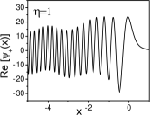
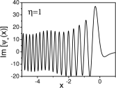
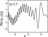
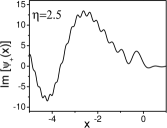
Figure 2: Real and imaginary part of $\psi_{+}$ as a function of $x$-coordinate for the case of the incident light hole. The top graphs refer to the large mixing between the hole branches ($\eta=1$) and the bottom graphs do to the small mixing ($\eta=2.5$).

Figure 2 shows the wave functions for the incident light hole for two different values of $\eta$ corresponding to large and small mixing between the two hole branches. High frequency oscillations correspond to the heavy hole component, which is obviously essential for $\eta=1$ and relatively small for $\eta=2.5$. Note that as was mentioned earlier at $\delta\to 0$ there appears a sharp resonance in the wave function near $x=0$. However it is hardly seen in the graphs. The reason is that the height of the peak, as it follows from (29, 30), is of the order $\delta^{-1/3}\exp(-2/9\,\eta^{3})$ and the peak itself exists only when $|\eta|\gg 1$. Real values of $\delta$ for the semiconductors are not less then $10^{-2}$, which is insufficient for observing the resonance.

In conclusion, the light-heavy hole transformation coefficient for reflection from a linear potential is found to be a function of a dimensionless parameter $\eta$, which is proportional to the longitudinal momentum of the light holes, and to be independent of the ratio of the light and heavy hole masses if this ratio is small. This function vanishes in both limits of large and small $\eta$, however the phases of light-light and heavy-heavy hole reflection coefficients are different in these limits. An approximate analytical expression for the transformation coefficient is found (see (47)). Account of the finite heavy hole mass is shown to be responsible for disappearance of an underbarrier resonance in the light hole wave function predicted in Suris .

After the paper was written authors became aware of the work Perel , where some of the results, in particular asymptotical expressions (43) and (44), were already obtained.

This work was partially supported by the Russian Foundation for Basic Research. One of the authors is grateful to I. Yu. Solov’ev for useful discussions.

References

• (1) M.I. Dyakonov, A.V. Khaetskii, Pis’ma Zh. Exp. Teor. Fiz. 33, 115, 1981(JETP Letters 33, 110, 1981).
• (2) R.A. Suris, Fiz. Tekh. Poluprovodn. 20, 2008, 1986 (Sov. Phys. Semicond. 20, 1258, 1986).
• (3) S.L. Chuang, Phys. Rev. B 40, 10379, 1989.
• (4) B.A. Foreman, Phys. Rev. B 49, 1757, 1994.
• (5) T. Kumar, M. Cahay, K. Roenker, Phys. Rev. B 56, 4836, 1997.
• (6) B.A. Foreman, Phys. Rev. B 56, R12748, 1997. XXXXXXXXXXXXXXXXXXXXX
• (7) M.V. Kisin, B.L. Gelmont, S. Luryi, Phys. Rev. B 58, 4605, 1998.
• (8) E.L. Ivchenko, A.Yu. Kaminski, U. Rossler, Phys. Rev. B 54, 5852, 1996.
• (9) B.A. Volkov, O.A. Pankratov, Pis’ma Zh. Exp. Teor. Fiz. 42, 145, 1985 (JETP Letters 42, 178, 1985).
• (10) A.V. Sokolskii, R.A. Suris, Sov. Phys. Semic., 5, 529, 1987.
• (11) P.C. Sercel and K.J. Vahala, Phys. Rev. B 42, 3690, 1990.
• (12) A.S. Polkovnikov and G.G. Zegrya, Phys. Rev. B 58, 4039, 1998.
• (13) V.L. Pokrovskii, I.M. Khalatnikov, Zh. Exp. Teor. Fiz. 40, 1713, 1961 (Sov. Phys. Jetp 13, 1207, 1961)
• (14) V.L. Ginzburg, Propagation of Electromagnetic Waves in Plasmas, Oxford: Pergamon Press, 1970.
• (15) Al.L. Efros and M. Rosen, Phys. Rev. B 58, 7120, 1998.
• (16) M.I. Dyakonov and V.I. Perel, Zh. Exp. Teor. Fiz. 92, 350, 1987 (Sov. Phys. Jetp 65, 200, 1987).