Evaluation of configurational entropy of a model liquid from computer simulations

Abstract

Computer simulations have been employed in recent years to evaluate the configurational entropy changes in model glass-forming liquids. We consider two methods, both of which involve the calculation of the ‘intra-basin’ entropy as a means for obtaining the configurational entropy. The first method involves the evaluation of the intra-basin entropy from the vibrational frequencies of inherent structures, by making a harmonic approximation of the local potential energy topography. The second method employs simulations that confine the liquid within a localized region of configuration space by the imposition of constraints; apart from the choice of the constraints, no further assumptions are made. We compare the configurational entropies estimated for a model liquid (binary mixture of particles interacting via the Lennard-Jones potential) for a range of temperatures, at fixed density.

1 Introduction

Whether a thermodynamic phase transition underlies the transformation of a supercooled liquid into an amorphous solid, or glass, at the laboratory glass transition temperature $T_{g}$ is among the central questions addressed by numerous researchers studying the supercooled liquid and glassy states. The notion of configurational entropy[1, 2] has played a significant role in attempts to define and understand the thermodynamic nature of the glass transition. In recent times, there have been various attempts to determine the configurational entropy of realistic liquids analytically and by computer simulations [3, 4, 5, 6, 8, 9, 10, 11, 12, 13, 14, 15, 16, 17]. The purpose of this paper is to compare two such methods that have been studied recently, namely the evaluation of the configurational entropy via the analysis of local potential energy minima or inherent structures (IS)[7, 8, 9, 10, 11, 16, 17], and by the calculation of basin free energies by confining the liquid within a localized region of configuration space by the imposition of constraints[6]. These approaches, and results from their implementation, are described in the following sections.

The model liquid studied is a binary mixture of $204$ type $A$ and $52$ type $B$ particles, interacting via the Lennard-Jones (LJ) potential, with parameters $\epsilon_{AB}/\epsilon_{AA}=1.5$, $\epsilon_{BB}/\epsilon_{AA}=0.5$, $\sigma_{AB}/\sigma_{AA}=0.8$, and $\sigma_{BB}/\sigma_{AA}=0.88$, and $m_{B}/m_{A}=1$, which has been extensively studied as a model glass former[18, 19, 8, 11, 17]. Results presented in Sec. II are from molecular dynamics simulations, at a reduced density $\rho=1.2$, which have been described in detail elsewhere[19, 17]. Since the density is fixed, the dependence on density is not always shown explicitly in the following.

2 Configurational Entropy from Inherent Structures

In the inherent structure approach[7], one considers the division of configurational space into basins of local potential energy minima. In practice such basins may be defined as the set of all points in configurational space that maps to the given local minimum under a specified local energy minimization procedure. Quite generally, one may then write the total partition function of the system as a sum of restricted partition function integrals over individual basins. Rewriting the partition function in this way introduces an entropy term associated with the number of local potential energy minima. With the expectation that configurations within a given basin are accessible to each other by thermal agitation while those belonging to distinct minima may not be, the number of distinct potential energy minima can be seen to be a measure of the number of physically distinct configurations or structures the system can adopt, i. e. a measure of the configurational entropy.

Thus, the canonical partition function is re-written as a sum over all local potential energy minima, which introduces a distribution function for the number of minima at a given energy:

$$Q_{N}(\rho,T)=\Lambda^{-3N}{1\over N_{A}!N_{B}!}\int d{\bf r}^{N}exp\left(-\beta\Phi\right)$$ (1)

$$=\sum_{\alpha}exp\left(-\beta\Phi_{\alpha}\right)\Lambda^{-3N}\int_{V_{\alpha}}d{\bf r}^{N}exp\left(-\beta(\Phi-\Phi_{\alpha})\right)$$

$$=\int d\Phi_{\alpha}~{}\Omega(\Phi_{\alpha})~{}exp\left(-\beta(\Phi_{\alpha}+Nf_{basin}(\Phi_{\alpha},T))\right)$$

$$=\int d\Phi_{\alpha}~{}exp\left(-\beta(\Phi_{\alpha}+Nf_{basin}(\Phi_{\alpha},T)-TS_{c}(\Phi_{\alpha}))\right)$$

where $\Phi$ is the total potential energy of the system, $\alpha$ indexes individual inherent structures, $\Phi_{\alpha}$ is the potential energy at the minimum, $V_{\alpha}$ is the basin of inherent structure $\alpha$, $\Omega(\Phi_{\alpha})$ is the number density of inherent structures with energy $\Phi_{\alpha}$, and the configurational entropy $S_{c}\equiv k_{B}\ln\Omega$ (Note that here $S_{c}$ is a function of energy; the equilibrium average of this quantity displayed in Fig. 4 as a function of temperature).

The probability of finding the system in the basin of an inherent structure of a given energy is given by the above as,

$$P(\Phi_{\alpha},T)={1\over Q_{N}(\rho,T)}exp\left(-\beta(\Phi_{\alpha}+Nf_{basin}(\Phi_{\alpha},T)-TS_{c}(\Phi_{\alpha}))\right).$$ (2)

The probability distribution $P$ can be obtained from computer simulations, and offers a means of obtaining $S_{c}$, provided one can estimate $Q_{N}$ (equivalently the free energy $A(\rho,T)$ of the system) and the basin free energy $f_{basin}(\Phi_{\alpha},T)$.

The free energy at any desired temperature is obtained from thermodynamic integration of pressure and potential energy data from MD simulations[8, 6]. The absolute free energy $A(\rho,T)$ of the system at density $\rho$ at a reference temperature $T_{r}=3.0$ is first defined in terms of the ideal gas contribution $A_{id}(\rho,T)$ and the excess free energy $A_{ex}(\rho,T)$ obtained by integrating the pressure from simulations:

$$A(\rho,T)=A_{id}(\rho,T)+A_{ex}(\rho,T),$$ (3)

$$\beta A_{id}(\rho,T)=N\left(3~{}\ln\Lambda+\ln\rho-1\right),$$

$$\beta_{r}A_{ex}(\rho,T_{r})=\beta_{r}A^{0}_{ex}(0,T_{r})+N\int_{0}^{\rho}{d\rho^{{}^{\prime}}\over\rho^{{}^{\prime}}}\left({\beta_{r}P\over\rho^{{}^{\prime}}}-1\right),$$

$$\beta_{r}A^{0}_{ex}(0,T_{r})=-\ln{N!\over N_{A}!N_{B}!}.$$

Here, $N$ is the number of particles, $\beta\equiv k_{B}T$, $\Lambda$ is the de Broglie wavelength, and $A^{0}_{ex}$ arises from the mixing entropy. $A_{ex}$ at a desired temperature may be evaluated by integrating the potential energy, $E$:

$$\beta A_{ex}(\rho,\beta)=\beta A_{ex}(\rho,\beta_{r})+\int_{\beta_{r}}^{\beta}E(\rho,\beta^{{}^{\prime}})d\beta^{{}^{\prime}}$$ (4)

As observed in [8, 11], the $T$ dependence of $E$ at the studied density is well described by the form $E(\rho,T)\sim T^{3/5}$, in agreement with predictions for dense liquids[20]. A fit of the potential energy data to this form affords a means of extending with confidence the temperature dependence of $E$ to $T$ values where direct MD data is unavailable.

The basin free energy $f_{basin}(\Phi_{\alpha},T)$ is obtained by a restricted partition function sum over a given inherent structure basin, $V_{\alpha}$. For sufficiently low temperatures, one may expect the basin to be harmonic to a good approximation. In the harmonic approximation, we have

$$\beta f={3\over 2}\ln({\beta\over 2\pi})+{1\over 2N}\sum_{i}^{3N-3}\ln\lambda_{i}\equiv\beta f_{therm}+\beta f_{vib},$$ (5)

where $\lambda_{i}$ are eigenvalues of the Hessian or curvature matrix at the minimum. For individual minima, these eigen values are obtained by numerical diagonalization of the Hessian. The basin free energy can then be obtained either as a function of the inherent structure energy (by averaging free energies within individual energy bins) or as a function of temperature, by averaging all inherent structures sampled at a given temperature. $\beta f_{vib}$ is a slowly varying function of temperature (the temperature dependence is obtained by averaging over $1000$, $100$ inherent structures at $T<1.$, $T>1.$ respectively), and is fitted to the form $\beta f_{vib}(T)=f_{0}+f_{1}/T^{2}$ which fits available data quite well.

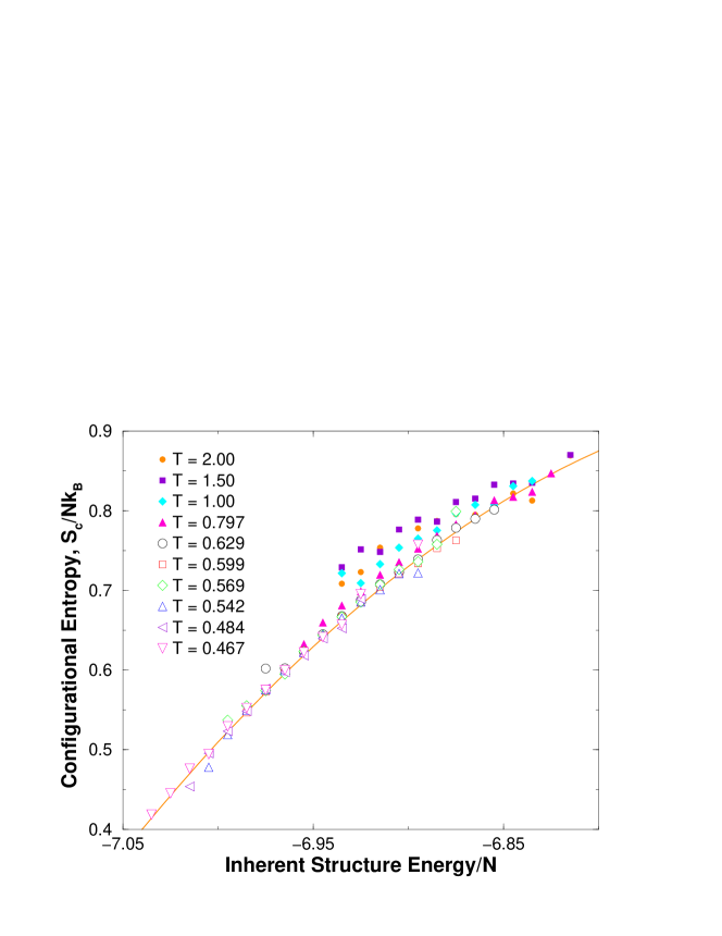
Figure 1: Configurational entropy as a function of inherent structure energy per particle, obtained from a range of temperatures. The overlap of curves for $T<0.8$ indicates that the harmonic approximation to the basin free energy is reasonable for $T<0.8$. The solid line is a quadratic fit.

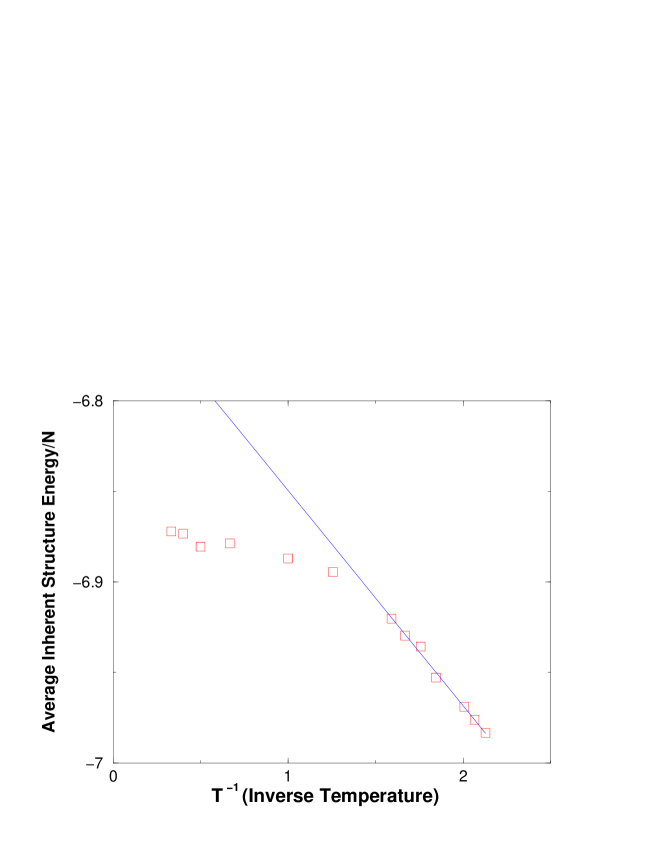
Figure 2: Average inherent structure energy vs. inverse temperature, showing that at low temperatures, the temperature dependence is well-described by $T^{-1}$ while above $T=0.8$ this dependence is not valid.

If the harmonic approximation to the basin free energy is accurate, inversion of Eq. (2), expressing $S_{c}(\Phi_{\alpha})$ in terms of $P(\Phi_{\alpha},T)$, $Q_{N}(\rho,T)$ (or $A(\rho,T)$) and $f_{basin}(\Phi_{\alpha},T)$, for different temperatures $T$, should result in curves that overlap with each other, as $S_{c}(\Phi_{\alpha})$ is independent of $T$. Figure 1 shows the result of such inversion, which indicates that below $T=0.8$, the various $S_{c}$ curves do overlap, while they do not at higher $T$. The procedure applied here is similar to, but improves upon, the procedure of shifting unnormalized $S_{c}$ curves adopted in [8, 10]. Thus, Fig. 1 indicates that a harmonic approximation to the basin free energy is not valid for temperatures higher than $T=0.8$. The temperature dependence of the average inherent structure energy $E_{IS}$, shown in Fig. 2, is consistent with this conclusion. As discussed in [10], a simple expectation for the T-dependence of the average inherent structure energy in the harmonic regime is that $E_{IS}\sim 1/T$. Figure 2 shows that such a T-dependence is indeed valid at low temperatures, but breaks down for $T>0.8$. However, this observation must be viewed in conjunction with two other observations about the topography of the inherent structure basins: (i) it has been demonstrated recently [21] that the separation between ‘vibrational’ and ‘inter-basin’ relaxation becomes reasonable for temperatures close to and below the mode coupling $T_{c}$ ($\sim 0.45$ for the model liquid studied here). (ii) The difference in the potential energy of instantaneous configurations and the corresponding inherent structures is nearly linear with a slope of $3/2$ for temperatures as high as $T=1.5$, as shown in Fig. 3. Such a linear temperature dependence would normally be associated with harmonic behavior, which in the present case is misleading.

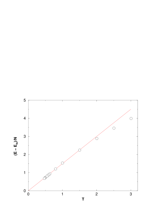
Figure 3: Temperature dependence of the difference between the potential energy of liquid configurations and their corresponding inherent structures, which is linear with a slope of $3/2$ upto very high temperatures.

The total entropy of the liquid $S$ as well as the basin entropy $S_{basin}$ are evaluated as a function of density and temperature from the total and basin free energies. The configurational entropy $S_{c}(\rho,T)$ and the ideal glass transition $T_{IG}(\rho)$ are then given by,

$$S_{c}(\rho,T)=S(\rho,T)-S_{basin}(\rho,T);S_{c}(\rho,T_{IG}(\rho))=0.$$ (6)

Figure 4 shows the configurational entropy so obtained as a function of $T$. By extrapolation, based on the assumption that the potential energy varied with temperature as $T^{3/5}$, the ideal glass transition occurs at $T=0.294$, in good agreement with estimates in [8, 11].

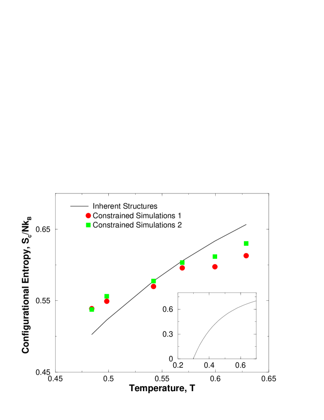
Figure 4: Configurational entropy vs. temperature, obtained from (a) Inherent structures (solid line), (b) constrained simulations, where the constraint is applied to equilibrated liquid configurations (filled circles, labeled ‘Constrained Simulations 1’), and (c) constrained simulations, where the constraint is applied to inherent structures (filled squares, labelled ‘Constrained Simulations 2’). Inset shows the extrapolation of $S_{c}$ which vanishes at $T=0.294$.

3 Constrained System Simulations

An alternate approach to defining the basin entropy, which has been explored by Speedy[6] is to impose constraints on a liquid to trap it in one of the basins it samples in equilibrium. A related approach has also been studied in [14]. With suitably chosen constraints, the calculated properties of the constrained system allow the evaluation of the basin entropy. A reasonable choice of constraint will restrict the system to a physically meaningful set of configurations related to each other without the need for configurational rearrangement. Further, such a constrained system should behave reversibly. In this work, the usefulness of one simple constraint is explored, by calculating the configurational entropy for a set of six temperatures at a fixed density of $1.2$, and compared with corresponding results from the inherent structure calculations described above. It is found that the constrained simulations result in comparable numbers for the configurational entropy from the inherent structure results.

Ten sample configurations are chosen at each temperature, and the Voronoi tessellation is performed for each configuration. The Voronoi cell of each given particle, and the corresponding geometric neighbors, correspond to the cage a particle experiences at short and intermediate time scales. A configurational rearrangement of particles in the system will result in a restructuring of the Voronoi tessellation as well. Thus, the constraint of restricting particles to their Voronoi cells is an a priori reasonable choice. Hence, a constraint is imposed which confines each particle to its Voronoi cell during the Monte Carlo simulation from which the properties of this constrained system are evaluated. Each Monte Carlo simulation mentioned below is performed for $25,000$ Monte Carlo steps. The constrained system can be studied at any desired temperature; the temperature of the simulation from which the reference configurations are taken will be referred to as the fictive temperature where there is need to distinguish these two temperatures. In order to estimate the configurational entropy, we must evaluate the free energy of the constrained system. This is done by thermodynamic integration[22, 23] from a reference system where each particle experiences a harmonic potential around the initial configuration (Einstein cystal). Considering a potential energy function of the form,

$$\Phi(\lambda,{\bf r}^{N})=(1-\lambda^{2})(\Phi_{LJ}({\bf r}^{N})+\Phi_{c})+\lambda^{2}C\sum_{i}({\bf r}_{i}-{\bf r}_{i}^{0})^{2}$$ (7)

where $\lambda$ is a tuning parameter that varies between $0$ and $1$, $\Phi_{LJ}$ is the Lennard-Jones potential of the unconstrained system, $\Phi_{c}$ is the constraining potential (which is zero if the constraint is obeyed and infinity if it is not), the corresponding free energy is given by

$$A(\lambda,\rho,T)=-k_{B}T\log\left[\Lambda^{-3N}\int d{\bf r}^{N}\exp(-\beta\Phi(\lambda,{\bf r}^{N}))\right].$$ (8)

The required free energy, $A(\lambda=0,\rho,T)$ is related to that of the Einstein crystal (which may be calculated straightforwardly), by

$$A(\lambda=0,\rho,T)=A(\lambda=1,\rho,T)-\int_{0}^{1}{\partial A\over\partial\lambda}~{}d\lambda$$ (9)

where, from differentiating Eq. (8) with respect to $\lambda$,

$${\partial A\over\partial\lambda}=-2\lambda<\Phi_{LJ}-C\sum_{i}({\bf r}_{i}-{\bf r}_{i}^{0})^{2}>.$$ (10)

The required average in the above equation is calculated by performing Monte Carlo simulations for a set of $11$ $\lambda$ values. The values of $\partial A/\partial\lambda$ obtained are shown in Fig. 5. The free energy for $\lambda=1$ is

$$A(\lambda=1,\rho,T)=3Nk_{B}T\left[\log\Lambda-{1\over 2}\log({\pi\over\beta C})\right].$$ (11)

All the above calculations are also performed using the inherent structures corresponding to the equilibrated liquid configurations mentioned above. With the free energy of the liquid evaluated as described in the previous section and the free energy of the constrained system obtained as described here, the configurational entropy of the system is given by

$$S_{c}/k_{B}={A_{cs}\over Nk_{B}T}-{A\over Nk_{B}T}$$ (12)

where $A_{cs}$ is the free energy of the constrained system. The resulting configurational entropies are shown in Fig. 4. The $S_{c}$ values from the constrained system simulations are comparable with the inherent structure results, but the agreement is moderate. In particular, the constrained system results vary more weakly with temperature.

To verify that the chosen constraint is a reasonable one, the free energies of the constrained system (for configurations from equilibrium runs at (fictive) temperatures $T_{f}=0.629,0.484$) are obtained independently at $T=0.1$ and $T=1.2$ from thermodynamic integration with respect to the Einstein crystal. Simulations are also performed for temperatures in between these two values, from which the temperature dependence of the potential energy is obtained. Using Eq. (4), $A(T=0.1)/Nk_{B}T$ is calculated by integrating from $T=1.2$. The difference of the directly calculated value and the one by integration is found to be $-0.0197$ for $T_{f}=0.484$ and $.0247$ for $T_{f}=0.629$. In other words, the constrained system appears to be reversible within the margin of error represented by these numbers. However, the discrepancy in the $S_{c}$ values between the constrained system and the inherent structure estimates is of the same order. Indeed, the discrepancy in the $S_{c}$ values for $T=0.484$ and $T=0.629$ is roughly the same as the discrepancy in the free energies above. It is likely that the sample of ten configurations used here is too small to obtain more accurate values.

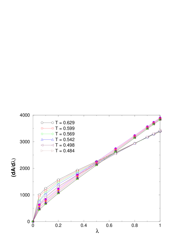
Figure 5: Values of ${\partial A\over\partial\lambda}$ for temperatures as marked. The filled symbols represent values for systems constrained with respect to the corresponding inherent structures.

4 Conclusions

Configurational entropy is obtained for a binary mixture liquid from analysis of inherent structures, and from estimation of the basin free energy via constrained system simulations. While the harmonic approximation used in the inherent structure approach to evaluate the basin free energy is in general questionable, the difficulty in the constrained system approach is the proper choice of constraint. The values for the configurational entropy obtained are comparable but show only moderate agreement. Further tests for the accuracy of the constrained system results, and more importantly, exploration of improved constraining methods are desirable for making a more stringent comparison of these two methods of calculating the configurational entropy.

5 Acknowledgments

Extremely useful discussions with Robin Speedy are gratefully acknowledged.

6 References

References

- [1] J.H. Gibbs and E. A. Di Marzio J. Chem. Phys. 28, 373 (1958).
- [2] G. Adam and J.H. Gibbs J. Chem. Phys. 43, 139 (1958).
- [3] R. J. Speedy, Mol. Phys. 80 1105 (1993).
- [4] R. J. Speedy and P. G. Debenedetti, it Mol. Phys. 81 237 (1994).
- [5] R. J. Speedy and P. G. Debenedetti, it Mol. Phys. 88 1293 (1996).
- [6] R. J. Speedy, J. Molec. Struct. 485-486 573 (1999).
- [7] F.H. Stillinger and T.A. Weber, Phys. Rev. A 25, 978 (1982); Science 225, 983 (1984); F.H. Stillinger, Science 267, 1935 (1995).
- [8] F. Sciortino, W. Kob and P. Tartaglia, Phys. Rev. Lett. 83, 3214 (1997).
- [9] F. Sciortino, W. Kob and P. Tartaglia, this volume.
- [10] S. Buechner and A. Heuer, Phys. Rev. E 60, 6507 (1999); Phys. Rev. Lett. 84, 2168 (2000).
- [11] B. Coluzzi, G. Parisi and P. Verrocchio, J. Chem. Phys. 112 2933 (2000).
- [12] A. Scala, F. W. Starr, E. La Nave, F. Sciortino and H. E. Stanley, Nature (in press) (2000); cond-mat/9908301.
- [13] L. Angelani, G. Parisi, G. Ruocco and G. Viliani, Phys. Rev. Lett. 81 4648 (1998).
- [14] M. Cardenas, S. Franz and G. Parisi, J. Phys. A: Math. Gen. 31, L163 (1998).
- [15] M. Mezard and G. Parisi, Phys. Rev. Lett. 82, 747 (1999); M. Mezard, Physica A 265, 352 (1999); M. Mezard and G. Parisi, J. Chem. Phys. 111, 1076 (1999).
- [16] B. Coluzzi, M. Mezard, G. Parisi and P. Verrocchio, J. Chem. Phys. 111, 9039 (1999); B. Coluzzi, G. Parisi and P. Verrocchio, Phys. Rev. Lett. 84, 306 (2000).
- [17] S. Sastry, Phys. Rev. Lett. (in press)
- [18] W. Kob and H. C. Andersen, Phys. Rev. E 51, 4626 (1995); K. Vollmayr, W. Kob and K. Binder J. Chem. Phys. 105, 4714 (1996).
- [19] S. Sastry, P. G. Debenedetti and F.H. Stillinger, Nature 393, 554 (1998).
- [20] Y. Rosenfeld and P. Tarazona, Mol. Phys. 95, 141 (1998).
- [21] T. B. Schröder, S. Sastry, J. Dyre and S. C. Glotzer, J. Chem. Phys 112 xxx (2000) (in press).
- [22] R. Speedy (unpublished).
- [23] D. Frenkel and A. J. C. Ladd, J. Chem. Phys. 81 3188 (1984).