Multi-Choice Minority Game

Abstract

The generalization of the problem of adaptive competition, known as the minority game, to the case of $K$ possible choices for each player is addressed, and applied to a system of interacting perceptrons with input and output units of the type of $K$-states Potts-spins. An optimal solution of this minority game as well as the dynamic evolution of the adaptive strategies of the players are solved analytically for a general $K$ and compared with numerical simulations.

I Introduction

Considerable progress in the theoretical understanding of market phenomena has been achieved by the study of the minority game. This prototypical model describes a system of agents interacting through a market mechanism [1, 2, 3, 4, 5, 6]. The game is based on the idea that the behavior of the agents is determined by the economic rule of supply and demand. According to this rule, given the available options (such as buy/sell), an agent wins if he chooses the minority action. The research of this game has been focused on cases in which each agent can choose between two options using its most efficient strategy, where the strategies remain unchanged throughout the game [1, 2, 3, 4, 5, 6]. However, in the real world, many situations of interest involve more than two decision options as well as agents with dynamic strategies. Making decisions like where to spend the summer vacation or which server to choose while surfing the web (or more generally, how to distribute data traffic in computer networks [7]) are only two among many common problems with more than two options. Therefore, it is tempting to investigate cases with more than two possible choices provided to agents with dynamic strategies. In a recent study of an extension in which each agent is equipped with a neural network for making his decision [8] it was shown that a certain updating rule of the strategies of the agents improves the efficiency of the market, which is measured by the global profit of the agents. In this paper we generalize the aforementioned work to a multi-choice minority game, namely a game with general $K$ decision states.

The multi-choice minority game consists of $N$ players (agents) and $K$ possible decisions. In each step, each one of the players chooses one of the $K$ states, aiming to choose the state with the smallest number of agents. For example, a situation may arise, in which there are several possible roads which lead from place A to place B, and each driver who wants to get from A to B chooses one of the available roads. Because drivers want to avoid traffic jams, they try to choose the least traveled roads, assuming that all the roads are of the same length. Similarly, one usually prefers to go to the bar with the smallest number of people in it. Occurring over and over again, the minority decisions in these and other similar situations generate time series whose term at time $t$, $x_{t}$, has an integer value between $1$ and $K$ according to the minority decision. In the original game, the information provided to each player is the history vector of size $M$, whose components are the last $M$ minority states.

The paper is organized as follows: In section II a multi-layer neural network and the dynamic evolution of its weights are introduced. For the clarity of the rest of the paper which is somewhat technical we briefly discuss the main findings and results. In section III the reference case of players with random strategies is solved analytically. In section IV the global profit of the players for the network with optimal strategies (weights) is solved analytically in the thermodynamic limit, and shown to be superior to a random decision. The analytical results are compared with simulations on finite systems. In section V, the suggested updating rules for the weights are examined analytically and are found to saturate asymptotically the optimal global profit. Finally, section VI is devoted to a short summary and an outlook.

II The model

While many strategies for the multi-choices minority game are conceivable, we study the following model which uses neural networks: each one of the $N$ players is represented by a perceptron of a size $M$. The weights belonging to the $i$th player are $\{w_{ij}\}$ where $j=1,...,M$. All $N$ perceptrons have a common input which consists of $M$ components $x_{1},~{}...,~{}x_{M}$, where each one of the components can take one of the $K$ integers, $1,~{}2,~{}...,~{}K$, with equal probability.

The dynamics are defined by the following steps. In the first step, each one of the perceptrons calculates the $K$ induced local fields. For instance, the field $h_{im}$ induced by the $m$th state on player $i$ is defined as the summation over all weights belonging to the $i$th perceptron with input equal to $m$:

$$h_{im}=\sum_{j=1}^{M}w_{ij}\delta_{x_{j},m}.$$ (1)

In the second step, each player chooses its state, $\{\sigma_{i}\}$, following the maximal induced field:

$$\sigma_{i}=\{k_{1}\mid\max_{m=1,..,K}h_{im}=h_{ik_{1}}\}.$$ (2)

where $\sigma_{i}$ is the output (chosen state) of $i$th perceptron. In the third step, the occupancy of each state is calculated:

$$N_{\rho}=\sum_{j=1}^{N}\delta_{\sigma_{j},\rho},$$ (3)

where it is clear that $\sum_{\rho}N_{\rho}=N$. The output $min$ of the network is the minority decision

$$min=\{\rho\mid\min_{m=1,..,K}N_{m}=N_{\rho}\},$$ (4)

The game can also be represented by a feedforward network $M:N:1$ ($M$ input units, $N$ hidden units and $1$ output). All units (input, hidden, output) are represented by $K$-states Potts-spins. The weights $\{w_{ij}\}$ are from the input units to the hidden units, and the weights from the hidden units to the output are all equal to $-1$. The dynamics of hidden and output units are similar to zero temperature dynamics of Potts-spin systems [9, 10], following the maximal induced field. The free parameters in our game are the $MN$ weights, $\{w_{ij}\}$, from the input to the hidden units. Their values will be determined by the strategy adopted by each one of the players. Our local dynamic rules are based on the generalization of the on-line Hebbian learning rule for $K=2$ [8] to general $K$-states Potts model with the following updating rule;

$$w_{ij}^{+}=w_{ij}+{{\eta}\over{M}}(K\delta_{x_{j},\min}-1)$$ (5)

where $\eta$ is the learning rate and the sign $+$ indicates the next time step. Note that all agents use the same rule for updating their strategy.

The score of the game is determined similarly to the Ising case. Players belonging to the minority ($N_{min}$ players) gain $Q_{+}$, while the other $N-N_{min}$ players gain $Q_{-}$, where $Q_{+}>Q_{-}$. Note that in most previous works $Q_{+}$ was chosen to be $1$ and $Q_{-}$ was chosen to be either $0$ or $-1$. The global profit in such cases is

$$U=Q_{-}N+(Q_{+}-Q_{-})N_{min}.$$ (6)

It is clear that the maximization of the global profit $U$ is equivalent to the maximization of $N_{min}$, which is bounded from above by $N/K$. Note that in the Ising case each player belongs either to the minority or to the majority, where in the Potts case the situation is more complex. The score may depend on the exact values of $\{N_{i}\}$ (the score decreases with $N_{\rho}$), hence the total profit $U=U(\{N_{i}\})$. In such a case the maximization of the total profit may differ from the maximization of $N_{min}$, and will be discussed briefly in the end of this paper.

Before we turn to discuss the guideline of the derivation of the results, which are more involved than for the Ising case, let us present the main results: (a) The score and the dynamics are formulated analytically for general $K$, the number of possible decisions. Exact results are obtained for $K\leq 6$ and asymptotically for $K\rightarrow\infty$. Results for intermediate values of $K$ are obtained from simulations. (b) A relaxation to the optimal score is achieved for small learning rates. (c) Regarding the optimal case, the deviation of minority group size from $N/K$ is found to be non-monotonic with $K$. (d) The total score is independent of the size of the history ($M$, the size of the input) available for the agents. (e) All agents are using the same type of dynamic strategy and gain on average (over time) the same profit. Our system does not undergo a phase transition to a state where the symmetry among the agents is broken into losers and winners [4, 5]. Throughout the investigation of the game we assume that the memory size $M$ is larger than the number of players $N$ (otherwise the completely symmetric Potts configuration is geometrically impossible). Albeit, simulations of the same dynamic for systems with $M<N$ show even better results for the global profit.

III The random case

In case where the maximization of the global profit $U$ is identical to the maximization of $N_{min}$, the quantity of interest is

$$<{\epsilon_{min}}^{2}>={1\over{N}}<(N_{min}-N/K)^{2}>,$$ (7)

where the symbol $<~{}~{}>$ indicates an average over input patterns, and $N/K$ is the average number of players in each state. Note that in our calculations the input vector presented to the players at each step of the game consists of random components[4, 8], instead of the true history. Nevertheless, simulations indicate that the system behavior is only slightly affected by the randomness of the inputs and the game properties remain similar.

For random players, each weight (among the $MN$ weights $\{w_{ij}\}$) is chosen from a given unbiased distribution and a variance $1/M$. Hence, the distribution of the overlap $R$ between weights belonging to any two players $\rho$ and $\phi$

$$R_{\rho\phi}=\sum_{j=1}^{M}w_{\rho j}w_{\phi j}$$ (8)

is a Gaussian with zero mean and variance $1/M$. In the thermodynamic limit and for $M>N$, one can show that in the leading order the overlap between each pair is an independent random variable. For random players and $K=2$ one finds $<\epsilon^{2}>=<\sum_{\rho}(N_{\rho}-N/K)^{2}/(NK)>=1/4$; however, for general $K$ even the derivation of a similar quantity is non-trivial. The two cornerstones of the calculations below are the probability of a microscopic configuration $P(\{\sigma_{i}\})$, and the degeneracy $D(\{N_{\rho}\})$ of a macroscopic configuration $\{N_{\rho}\}$, which is given by the multinomial coefficient:

$$D(\{N_{\rho}\})=\frac{N!}{\prod_{\rho}N_{\rho}!}.$$ (9)

In the large $N$ limit, the typical deviation of the size of each group from $N/K$ is expected to scale with $\sqrt{N}$. Hence we define:

$$N_{\rho}=N/K+\epsilon_{\rho}\sqrt{N}$$ (10)

where it is clear that $\sum_{\rho}\epsilon_{\rho}=0$ and without the loss of generality we assume $N_{min}=N_{1}\leq N_{\rho}~{}~{}\forall\rho>1$. Applying the Stirling approximation to Eq. (9) yields the degeneracy as a function of $\{\epsilon_{\rho}\}$:

$$D_{K}(\{\epsilon_{\rho}\})\sim K^{N}\exp({-{K\over 2}\sum_{\rho=1}^{K}\epsilon_{\rho}^{2}})\delta(\sum_{\rho=1}^{K}\epsilon_{\rho}).$$ (11)

If the average over $R_{\rho\phi}$, which we denote by $R$, is $0$, the agents make their choice independently and randomly, so each microscopic configuration has the same probability $P_{K}=(1/K)^{N}$. Now the average over $\epsilon_{min}^{2}$ can be evaluated:

$$<\epsilon_{min}^{2}>_{R}={\int_{-\infty}^{0}{\epsilon_{1}}^{2}d\epsilon_{1}\Pi_{\rho>1}\int_{\epsilon_{1}}^{\infty}d\epsilon_{\rho}D_{K}(\{\epsilon_{\rho}\})P_{K}(\{\epsilon_{\rho}\})\over\int_{-\infty}^{0}d\epsilon_{1}\Pi_{\rho>1}\int_{\epsilon_{1}}^{\infty}d\epsilon_{\rho}D_{K}(\{\epsilon_{\rho}\})P_{K}(\{\epsilon_{\rho}\})}.$$ (12)

The quantity $<{\epsilon_{min}}^{2}>_{R=0}$ was calculated numerically for $K=3,~{}4,~{}5,~{}6$ and found to be equal to $\sim 0.313,~{}0.322,~{}0.320,~{}0.309$, respectively (see Fig. 1). Results obtained from simulations with $N=5000$ and $K\leq 6$ are in an excellent agreement with Eq. (12). For $K>6$ the reported results in Fig. 1 were derived only from simulations and are in an excellent agreement with the asymptotic behavior of Eq. (12), $<\epsilon_{min}^{2}>_{R=0}\sim 2\log(K)/K$. Another quantity of interest is the average deviation of the average number of players in each state from $N/K$, $<\epsilon^{2}>=<{1\over{K}}\sum_{\rho}\epsilon_{\rho}^{2}>$. Similarly to Eq. (12), this quantity can be derived analytically and gives

$$<\epsilon^{2}>_{R=0}={{K-1}\over{K^{2}}}.$$ (13)

FIG. 1.: Simulations for $<{\epsilon_{min}}^{2}>$ as a function of $K$ for both the optimal case $R=-{1\over{N-1}}$ (solid curve) and the random case $R=0$ (long dashed curve). Analytical results up to $K=6$ agree with simulations for both $R=-{1\over{N-1}}$ (filled circles) and $R=0$ (triangles). Inset: $\Gamma_{K}=<{\epsilon_{min}}^{2}>_{R=0}/<{\epsilon_{min}}^{2}>_{R=-{1\over{N-1}}}$ as a function of $K$.

IV The optimal case

So far we have compared $<{\epsilon_{min}}^{2}>$ and $<{\epsilon}^{2}>$ for random players, where the average overlap is zero. Without breaking the symmetry among the players, the weights can be represented by $N$ weight vectors which are symmetrically spread around their center of mass. More precisely, we denote the weight vector of the $i$th perceptron as ${\bf w}_{i}$, and assume that it can be expressed as

$${\bf w}_{i}={\bf C}+{\bf g}_{i},$$ (14)

where the center of mass ${\bf C}\equiv{1\over N}\sum_{i}{\bf w}_{i}$, and $\{{\bf g}_{i}\}$ are $N$ unit vectors of rank $M$ obeying the symmetry

$${\bf g}_{i}\cdot{\bf g}_{j}=(1+{{1}\over{N-1}})\delta_{ij}+{{1}\over{N-1}}.$$ (15)

Hence, the total profit and $N_{min}$ are functions of only one parameter, $C$. It is clear that the maximization of the total profit or $N_{min}$ (as for the case $K=2$) is obtained when $C=0$, which is the maximal achievable homogeneous repulsion among $N$ vectors of rank $M>N$. The repulsion is the natural tendency of each player in the minority game, since the goal is to act differently than other players. Without a cooperation which breaks the players into sub-groups, the maximal homogeneous repulsion is $R=-1/(N-1)$.

The two questions of interest are the following: (a) What is $<\epsilon^{2}>$ and $<{\epsilon_{min}}^{2}>$ as a function of $K$ for the optimal solution, $C=0$ and $R=-1/(N-1)$? (b) Is the optimal solution achievable by local dynamic rules for each one of the players? We first examine the former question regarding the optimal solution, and then we turn to study the dynamic behavior of the players.

The average deviation of the number of players in each state from $N/K$ at $C=0$ and for $R=O(1/N)$ can be calculated analytically. The main idea is that this quantity can be calculated similarly to Eq. (12), or via $<{\epsilon}^{2}>={1/(NK)}<(\sum_{\rho=1}^{K}\sum_{i=1}^{N}\delta_{\sigma_{i},\rho}-{N/K})^{2}>$. The simplification of the later expression is such that an average over only a pair of players has to be done. The result as a function of $K$ gives

$$<{\epsilon}^{2}>_{R}={{K-1}\over{K^{2}}}+R(N-1)(K-1)K\mu,$$ (16)

where $\mu=[\int_{-\infty}^{\infty}{e^{-h^{2}}\over{2\pi}}{(1-H(h))}^{K-2}dh]^{2}$ and $H(x)=0.5\;\mbox{erfc}({x\over\sqrt{2}})$.

Regarding the optimal score, the quantity of a particular interest is $<{\epsilon}_{min}^{2}>_{R={{-1}\over{N-1}}}$. This quantity has to be compared with $<{\epsilon}_{min}^{2}>_{R=0}$ in order to estimate the improvement in the average global gain relative to the random case. Note that the calculation of Eq. (12) for $R\neq 0$ is nontrivial since $P_{K}(\{\epsilon_{\rho}\})$ is no longer independent of the configuration $\{\epsilon_{\rho}\}$. However, we can overcome this difficulty in the following way. For $R=O(1/N)$ one can show that in the leading order $P_{K}(\{\epsilon_{\rho}\})$ has the same form as $D_{K}(\{\epsilon_{\rho}\})$:

$$P_{K}(\{\epsilon_{\rho}\})\sim({1/K})^{N}\exp({-{A(R)}\sum_{\rho=1}^{K}\epsilon_{\rho}^{2}})\delta(\sum_{\rho=1}^{K}\epsilon_{\rho}),$$ (17)

where the exact value of $A(R)$ is unknown. The observation that both $P_{K}(\{\epsilon_{\rho}\})$ and $D_{K}(\{\epsilon_{\rho}\})$ have the same dependence on $\{\epsilon_{\rho}\}$ (Eqs. (11) and (17)) indicates that the ratio $<\epsilon_{min}^{2}>/<\epsilon^{2}>$ is independent of $R$ if $R=O(1/N)$, and in particular:

$${<{\epsilon}^{2}>_{R=0}\over{<{\epsilon_{min}}^{2}>}_{R=0}}={<{\epsilon}^{2}>_{R=-{1\over{N-1}}}\over{<{\epsilon_{min}}^{2}>}_{R=-{1\over{N-1}}}}=\beta_{K}.$$ (18)

This property can be easily derived by rescaling $\epsilon_{\rho}\to\sqrt{A(R)}\epsilon_{\rho}$ in the integral representation (Eq. (12)) of each one of the four terms in Eq. (18). The same prefactor appears both in the denominator and in the numerator, and the dependence of $\beta_{K}$ on $R$ via $A(R)$ is cancelled out. Using Eq. (18), ${<{\epsilon_{min}}^{2}>}_{R=-{1\over{N-1}}}$ can be obtained indirectly from the knowledge of the other three terms, which are given by Eqs. (12), (13), and (16). Results for ${<{\epsilon_{min}}^{2}>}_{R=-{1\over{N-1}}}$ are presented in Fig. 1. In order to confirm our analytical results we performed simulations for the optimal case, Eqs. (16) and (18), with $C=0$. The simulations were done in two stages. In the first stage, $N$ normalized vectors of rank $M$, obeying the constraints that the overlap among each pair is equal to $-1/(N-1)$, are generated using a recursive process. The details of the algorithm will be given elsewhere [11]. In the second stage, $<{\epsilon_{min}}^{2}>$ and $<{\epsilon}^{2}>$ were averaged over about $10^{5}$ randomly chosen inputs for a system with $N=400$ and $M=5000$. An excellent agreement between simulations and analytical results was obtained (see Fig. 1). The improvement in the global gain can be measured by the ratio $\Gamma_{K}=<{\epsilon_{min}}^{2}>_{R=0}/<{\epsilon_{min}}^{2}>_{R={-1\over{N-1}}}$. This ratio decreases monotonically with $K$ such that its maximal value $\Gamma_{2}=2.7548$ and for $K\to\infty$ $\Gamma_{K}\to 1$ (inset of Fig. 1).

V The dynamics which lead to the optimal solution

So far we derived the properties of the optimal solution for different values of $K$. Now we are turning to the second question: is the optimal solution achievable by local dynamic rules (Eq. (5))? After averaging Eq. (5) over $j$ and in the limit where the number of examples, $\alpha{M}$, scales with the number of input units $M$, one can find the following equation of motion for the center of mass

$${{dC^{2}}\over{d\alpha}}=2\eta{K}<\sum_{j}C_{j}\delta_{x_{j},min}>+\eta^{2}(K-1),$$ (19)

where $<~{}~{}>$ denotes an average over the random examples. For large $M$, in the leading order each input vector divides each weight vector into $K$ equal groups of size $M/K$. The minority state is the one whose group of weights gives the minimal sum. Using Eq. (19) and $M,N\to\infty$, $<\sum_{j}C_{j}\delta_{x_{j},min}>$ is the average minimal sum of a set of $M/K$ center of mass components, $\{C_{j}\}$. These $M/K$ quantities are random variables with zero mean and variance $C^{2}/M$ ( $<\sum_{j=1}^{M/K}C_{j}>=0$ and $<(\sum_{j=1}^{M/K}C_{j})^{2}>=C^{2}/K$). One can find that $<\sum_{j}{C_{j}\delta_{x_{j},min}}>$ is equal to

$${C\over{2}}(K-1)\sqrt{K\over{\pi}}\int_{-\infty}^{\infty}{e^{-y^{2}/2}\over\sqrt{2\pi}}[H({y\over{\sqrt{2}}})]^{K-2}dy.$$ (20)

Hence, for a given $K$, Eqs. (19) and (20) indicate a linear relation between the fixed point value of $C$ and the learning rate $\eta$ with corrections of $O(1/\sqrt{N})$. As $\eta\to 0$, $C\to 0$ and the system approaches the optimal configuration. The interplay between $C$ and $\eta$ was confirmed by simulations, where finite size effects decay as the size of the system becomes larger. This effect is depicted in Fig. 2 for $K=3$. The explicit dependence of $<{\epsilon_{min}}^{2}/N>_{R}$ on $C$ can be found for $R\sim O(1/N)$ via the relation

$$R={{C^{2}-{1\over{N-1}}}\over{C^{2}+1}}.$$ (21)

Results of simulations for $<{\epsilon_{min}}^{2}>_{R}$ as a function of $C$ for $N=103$ and $M=200$ are presented in the inset of Fig. 2. An excellent agreement between the analytical prediction and simulations was obtained in the regime of $C\sim O(1/\sqrt{N})$ (corresponding to $R\sim O(1/N)$).

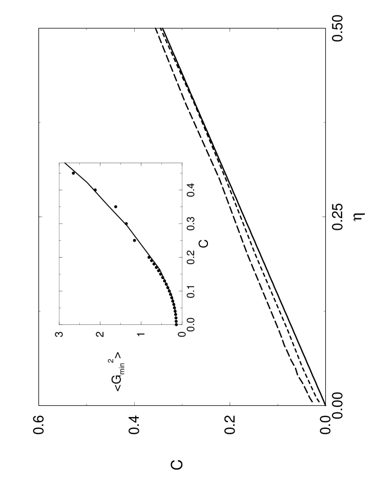
FIG. 2.: C as a function of $\eta$ for $K=3$. Analytical results (solid line) and simulations for $N=103$, $M=200$ (long-dashed), and for $N=400$, $M=403$ (dashed-line). Inset: $<{\epsilon_{min}}^{2}>$ as a function of $C$ for $K=3$. Analytical results (solid line) and simulations for $N=103$, $M=200$ (filled circles).

Note that although the global gain $U$ which corresponds to the Boolean case is monotonic with $K$, the non-monotonic behavior of ${\epsilon_{min}}$ implies that for non-Boolean cases non-monotonic behavior of $U$ may be obtained.

VI summary and outlook

In this paper we introduced a generalization of the minority game to the case of multi-choice. The problem was applied to a multilayer network with updating rules for the weights (strategies). Static and dynamic properties of the strategies were solved analytically for various $K$’s and were found to be in a good agreement with simulations on finite systems. This modification of the minority game to the case of multi-choice open a manifold of new questions, which certainly deserve future research. We have chosen two of those questions to briefly discuss here.

Firstly, as we have pointed out before, the function according to which the profit is awarded is not necessarily Boolean as in Eq. (6). In fact, the model is more realistic when the profit of a player is related to the size of his group, as well as to the size of the other groups [12]. Our analysis can be applied to these cases if the maximization of the global gain is equivalent to the maximization of the minority group. However, other scores may not fulfill this required condition. In these cases, it has to be determined whether the optimal symmetric configuration remains the maximal repulsion.

Secondly, the other strategies for the minority game that have been studied can be generalized to multi-choice situations in a straightforward manner: in the original game [1, 2, 5, 6] where each player has several decision tables, each table entry is now a value between $1$ and $K$. In Johnson’s stochastic strategy [13, 14], each player has a probability of choosing the outcome that was successful the last time, or to pick one of the others with equal probability. In the strategy of Reents [15], players who were not in the minority could switch to some other action with a small probability in the next time step. Similarly, other conceivable strategies can also be generalized. Preliminary checks imply that all these modified strategies show similar behavior compared to that of the binary-choice game, even though their theoretical treatment probably becomes more involved. While outcomes of these games certainly have to be measured against the reference values given in Eqs. (12) and (13), it is not clear under what circumstances relations like Eq. (18) hold for other strategies.

I. K., W. K. and R. M. acknowledge a partial support by GIF.

2

REFERENCES

- [1] D. Challet and Y. C. Zhang, Physica A 246, 407 (1997).
- [2] D. Challet and Y. C. Zhang, Physica A 256, 514 (1998).
- [3] R. Savit, R. Manuca and R. Riolo, Phys. Rev. Lett. 82, 2203 (1999).
- [4] A. Cavagna, J. P. Garrahan, I. Giardina and D. Sherrington, Phys. Rev. Lett. 83, 4429 (1999).
- [5] D. Challet, M. Marsili and R. Zecchina, Phys. Rev. Lett. (in press).
- [6] M. Marsili, D. Challet and R. Zecchina, cond-mat/9908480.
- [7] D. H. Wolpert, K. Tumer and J. Frank, electronic preprint, cs.LG/9905004.
- [8] R. Metzler, W. Kinzel and I. Kanter, Phys. Rev. E 62, 2555 (2000).
- [9] I. Kanter, Phys. Rev. A. 37, 2739, (1988).
- [10] T. L. H. Watkin, A. Rau, D. Bolle and J. van Mourik, J. Phys. I France 2, 167, (1992).
- [11] L. Ein-Dor, unpublished.
- [12] Y. Li, A. VanDeemen and R. Savit, Physica A 284, 461 (2000).
- [13] N. F. Johnson, P. M. Hui, R. Jonson and T. S. Lo, Phys. Rev. Lett. 82, 3360 (1999).
- [14] T. S. Lo, P. M. Hui and N. F. Johnson, cond-mat/0003379 (2000).
- [15] G. Reents, R. Metzler, W. Kinzel, cond-mat/0007351 (2000).
2