LUDWIG: A parallel Lattice-Boltzmann code for complex fluids

Abstract

This paper describes Ludwig, a versatile code for the simulation of Lattice-Boltzmann (LB) models in 3-D on cubic lattices. In fact Ludwig is not a single code, but a set of codes that share certain common routines, such as I/O and communications. If Ludwig is used as intended, a variety of complex fluid models with different equilibrium free energies are simple to code, so that the user may concentrate on the physics of the problem, rather than on parallel computing issues. Thus far, Ludwig’s main application has been to symmetric binary fluid mixtures. We first explain the philosophy and structure of Ludwig which is argued to be a very effective way of developing large codes for academic consortia. Next we elaborate on some parallel implementation issues such as parallel I/O, and the use of MPI to achieve full portability and good efficiency on both MPP and SMP systems. Finally, we describe how to implement generic solid boundaries, and look in detail at the particular case of a symmetric binary fluid mixture near a solid wall. We present a novel scheme for the thermodynamically consistent simulation of wetting phenomena, in the presence of static and moving solid boundaries, and check its performance.

1 Objectives

The objective of the work described here has been to develop a general purpose parallel Lattice-Boltzmann code (LB), called Ludwig, capable of simulating the hydrodynamics of complex fluids in 3-D. Such a simulation program should eventually be able to handle multicomponent fluids, amphiphilic systems, and flow in porous media as well as colloidal particles and polymers. In due course we would like to address a wide variety of these problems including detergency, binary fluids in porous media, mesophase formation in amphiphiles, colloidal suspensions, and liquid crystal flows. So far, however, we have restricted our attention to simple binary fluids, and it is this version of the code that will be described below in more detail. Nonetheless, the generic elements related to the structure of the code are valid for any multicomponent fluid mixture, as defined through an appropriate free energy, expressed as a functional of fluid density and one or more composition variables (scalar order parameters). We discuss in some detail also how to include solid objects, such as static and moving walls and/or freely suspended colloids, in contact with a binary fluid. More generally, the modular structure of Ludwig facilitates its extension to many other of the above problems without extensive redesign. But note that, with several of these problems (such as liquid crystal flows which require tensor order parameters), it is not yet clear how to proceed even at the serial level, and only first attempts have begun to appear in the literature Julia_prep .

2 Lattice Boltzmann model

The Lattice-Boltzmann model (LB) simulates the Boltzmann equation with linearized collisions on a lattice Higuera . Both the changes in position and velocity are discretized. It can be shown that, at sufficiently large length and time scales, LB simulates the dynamics of nearly incompressible viscous flows Qian92 ; Ladd94 . For the simplest case of a one-component fluid, it describes the evolution of a discrete set of particle densities on the sites (or nodes) of a lattice:

$$f_{i}(\vec{r}+\vec{c}_{i},t+1)-f_{i}(\vec{r},t)=-\omega\left(f^{\mathrm{eq}}_{i}(\vec{r},t)-f_{i}(\vec{r},t)\right)$$ (1)

The quantity $f_{i}(\vec{r},t)$ is the density of particles with velocity $\vec{c}_{i}$ resident at node $\vec{r}$ at time $t$. This particle density will, in unit time increment, be convected (or propagate) to a neighboring site $\vec{r}+\vec{c}_{i}$. Here $\vec{c}_{i}$ is a lattice vector, or link vector, and the model is characterized by a finite set of velocities $\{\vec{c}_{i}\}$. The quantity $f^{\mathrm{eq}}_{i}(\vec{r},t)$ is the ‘equilibrium distribution’ of $f_{i}(\vec{r},t)$, and is one of the key ingredients of the model. It characterizes the type of fluid that Ludwig will simulate, and determines the equilibrium properties of such a fluid (see section 2.1 below). The right hand side of equation 1 describes a mixing of the different particle densities, or collision: the $f_{i}$ distribution relaxes towards $f_{i}^{\mathrm{eq}}$ at a rate determined by $\omega$, the relaxation parameter. The relaxation parameter is related (through $\eta=(2\omega^{-1}-1)/6$) to the viscosity $\eta$ of the fluid, and gives us control of its dynamics.

To specify a particular model, besides the equilibrium properties given through $f^{\mathrm{eq}}$, one has to choose the geometry of the lattice in which the density of particles move. Such a geometry should specify both the arrangement of nodes and the set of allowed velocities. The only restrictions in such a choice lie on the fact that they should have sufficient symmetry to ensure that at the hydrodynamic level the behavior is isotropic and independent of the underlying lattice Wolfram86 . The hydrodynamic quantities, such as the local density, $\rho$, momentum, $\rho{\bf v}$ and stress, $\mathcal{P}_{\alpha\beta}$ are given as moments of the densities of particles $f_{i}(\vec{r},t)$ Qian92 ; Ladd94 , namely $\sum_{i}f_{i}=\rho$, $\sum_{i}f_{i}{\vec{c}_{i}}=\rho{\vec{v}}$, and $\sum_{i}f_{i}c_{i\alpha}c_{i\beta}=\mathcal{P}_{\alpha\beta}$.

The dynamics of LB, as expressed in equation 1, provides immediate insight into the implementation and underlying optimization issues. It is characterized by two basic dynamic stages:

• the propagation stage (left-hand side of equation 1), consisting of a set of nested loops performing memory-to-memory copies;

• the collision stage (right hand side), which has a strong degree of spatial locality and relies on basic add/multiply operations: its implementation is straightforward and can be highly optimized.

2.1 Binary fluid mixtures

The LB model described so far can be extended to describe a binary mixture of fluids, of tunable miscibility, by adding a second distribution function, $g_{i}$Swift . (Further distribution functions would allow still more complicated mixtures to be described.) As in single-fluid LB, the relevant hydrodynamic variables related to the order parameter are also moments of the additional distribution function $g_{i}$, namely the composition (order parameter) $\phi=\sum_{i}g_{i}$, and the flux $\sum_{i}g_{i}{\vec{c}_{i}}=\phi{\vec{v}}$. For each site (including solid sites), the distributions $f_{i}$ and $g_{i}$ are stored in a structure element of type Site:

typedef struct{
	Float f[NVEL],
		g[NVEL];
} Site;

where NVEL is the number of velocity vectors used by the model. For example, for the cubic lattices described later on, where Ludwig has been implemented so far, the number of velocity vectors has been 15 and 19. Figure 1 shows the sets of velocities for the two 3-D models developed.

Figure 1: D3Q15 (left) and D3Q19 (right) models. The D3Q15 model has fifteen velocities: one with speed zero (a rest particle), six with $(speed)^{2}=1$ (to nearest neighbors), and eight with $(speed)^{2}=3$ (to next next nearest neighbors). The D3Q19 model has nineteen velocities: one with speed zero (a rest particle), six with $(speed)^{2}=1$ (to nearest neighbors), and 12 with $(speed)^{2}=2$ (to next nearest neighbors).

We follow the procedure of Swift et al. Swift (see also Grubert for a schematic description) in which $f_{i}$ describes the density field $\rho$, whilst $g_{i}$ describes the order parameter field, $\phi$. Both distribution functions have relaxational dynamics of the type of equation 1 but are characterized by different relaxation parameters $\omega_{\rho,\phi}$. The second relaxation parameter, associated with the order parameter field, will determine its diffusivity. By studying appropriate moments of the distribution functions, one can construct a relaxational dynamics that will describe, in the continuum limit, the dynamics of a near-incompressible, isothermal binary fluid with an arbitrary local free energy functional $F[\phi]$. The model chosen is a symmetric ‘$\phi^{4}$’ or Cahn-Hilliard type free energy:

$$F=\int\mathrm{d}{\mathbf{r}}\left\{\frac{A}{2}\phi^{2}+\frac{B}{4}\phi^{4}+\frac{\kappa}{2}|\nabla\phi|^{2}\right\}$$ (2)

where $A$, $B$ and $\kappa$ are model parameters. For the density $\rho$, LB dynamics ensures an ideal gas equation of state, with a speed of sound equal to $1/\sqrt{3}$ . In practice $\rho$ remains almost constant at a value which we choose to be unity. This can be done by ensuring that under all conditions the fluid velocity remains small compared to unity in lattice units. (More generally one requires velocities small compared to the sound speed.) For negative $A$, the above model has two coexisting fluid phases with order parameter values $\pm\phi^{*}$; for many problems it is convenient to set $B=-A$ so that $\phi^{*}=1$.

Note also that, although there is a long history of studying $\phi^{4}$ theory on the lattice, one needs to be aware of possible lattice artifacts in the thermodynamic, as well as the hydrodynamic, sectors of the model Kendon00 . For example, the coefficient $\kappa$, determines the thickness $\xi_{0}=(\kappa/2|A|)^{1/2}$ and the interfacial tension $\sigma=(8\kappa|A|^{3}/9B^{2})^{1/2}$ of the interface between two fluids Swift . But the thickness must be kept large enough to avoid a strong anisotropy of the interfacial tension caused by the underlying lattice. Moreover, the values of the different parameters should be carefully selected to give the required compromise between numerical stability and accuracy, and computational speed Kendon00 . However, since the same physical parameters (in a binary fluid, viscosity, density, interfacial tension) can be achieved with more than one set of simulation parameters, it is normally possible to steer around any problems, though they do present traps for the unwary. The specific role played by order parameter mobility in the simulations of binary fluids is discussed in Kendon00 ; Kendon99 .

We emphasize that Ludwig is structured so that the free energy functional can be chosen at will. This is a desirable feature of LB over, for example, the dissipative particle dynamics algorithm (DPD), where the free energy being modeled has to be deduced a posteriori from the simulation results Groot , although first attempts are being carried out to allow for free energy a priori determination Daan . The user of the code has to evaluate, from the free energy and according to a well-established procedure Swift ; Kendon00 , the equilibrium distribution functions $f_{i}^{\mathrm{eq}}$, $g_{i}^{\mathrm{eq}}$ for use in the relaxation equation 1 and the corresponding one for $g_{i}$. This data is entered into the subroutine for the collision step. For example, in the case of the binary fluid mixture in the D3Q15 geometry one has Kendon00

$$f_{i}^{\mathrm{eq}}=\rho\omega_{\nu}\left\{A_{\nu}+3v_{\alpha}c_{i\alpha}+\frac{9}{2}v_{\alpha}v_{\beta}c_{i\alpha}c_{i\beta}-\frac{3}{2}v^{2}+G_{\alpha\beta}c_{i\alpha}c_{i\beta}\right\}.$$ (3)

Here, ${\nu}$ is an index that denotes the speed, $|{\vec{c}}_{i}|=0,1,3^{1/2}$, and $\omega_{\nu}$, $A_{\nu}$ and $G_{\alpha\beta}$ are constants given by

$$\omega_{0}=2/9;\;\;\;\omega_{1}=1/9;\;\;\;\omega_{3}=1/72,$$ (4)

$$A_{0}=\frac{9}{2}-\frac{7}{2}\mathrm{Tr}\mathcal{P}^{\mathrm{th}};\;\;\;A_{1}=A_{3}=\frac{1}{\rho}\mathrm{Tr}\mathcal{P}^{\mathrm{th}},$$ (5)

$$G_{\alpha\beta}=\frac{9}{2\rho}\mathcal{P}^{\mathrm{th}}_{\alpha\beta}-\frac{3\delta_{\alpha\beta}}{2\rho}\mathcal{P}^{\mathrm{th}}.$$ (6)

Here $\mathcal{P}^{\mathrm{th}}_{\alpha\beta}$ is the thermodynamic contribution to the pressure tensor which can be evaluated directly from the chosen form of the free energy functional Swift , and for equation 2 it reads

$$\mathcal{P}^{\mathrm{th}}_{\alpha\beta}=\left\{\frac{\rho}{3}+\frac{A}{2}\phi^{2}+\frac{3B}{4}\phi^{4}-\kappa\phi\nabla^{2}\phi-\frac{\kappa}{2}(\nabla\phi)^{2}\right\}\delta_{\alpha\beta}+\kappa(\partial_{\alpha}\phi)(\partial_{\beta}\phi).$$ (7)

The equilibrium distribution for the order parameter, $g_{i}^{\mathrm{eq}}$, is the same as for $f_{i}^{\mathrm{eq}}$, with $\mathcal{P}^{\mathrm{th}}_{\mu\nu}$ replaced by $\tilde{M}\mu\,\delta_{\mu\nu}$ in the above equations; here $\tilde{M}(\omega_{\phi}^{-1}-1/2)=M$, where $M$ is the order parameter mobility Kendon00 .

2.2 Gradient discretization

For evaluation of $\mathcal{P}^{\mathrm{th}}_{\alpha\beta}$ and other quantities, we need to compute spatial gradients of $\phi$. To minimize thermodynamic lattice anisotropies, this is done using a larger set of links than used for the propagation step; for example on the D3Q15 lattice we use all 26 (first, second and third) nearest neighbors so that numerically

$$\partial_{\alpha}\phi(\mathbf{x})=\frac{\sum_{i}c_{i\alpha}\phi(\mathbf{r}+\mathbf{c}_{i})}{\sum_{i}c_{i\alpha}c_{i\alpha}}$$ (8)

$$\nabla^{2}\phi(\mathbf{r})=\frac{1}{9}\left[\left(\sum_{i=1}^{26}\phi(\mathbf{r}+\mathbf{c}_{i})\right)-26\phi(\mathbf{r})\right]$$ (9)

with an enlarged set $\{{\vec{c}}_{i}\}$. Note that these are not the only possible choices. There may be considerable scope for further improvement by optimizing the choices made for gradient discretization, but we leave this for future work.

2.3 Numerical stability

One drawback of LB is that, unlike DPD and some other competing mesoscale techniques, it is not unconditionally stable. However, our experience suggests that even if the model becomes eventually unstable for any given set of parameter values, the problem arises so suddenly that such an instability does not impede collection of robust and reliable data over long periods beforehand Kendon00 . Nonetheless, it would be very desirable to have a fully stable version of the algorithm and this might considerably reduce the time spent in parameter steering exercises that are currently needed prior to allocating resources for production runs.

3 Implementation details

3.1 Users’ requirements

The scientific objectives presented in section 1 are ambitious and imply the availability of a variety of different features, consistent with a development time stretching across a few years. Because none of the LB codes available at the start of the project had the required features, Ludwig’s creators decided to design a new package from scratch whose main characteristic would be its versatility: Ludwig had to be capable of producing data of scientific interest at an early stage of its development, include built-in support for multiple models and free energies, and be sufficiently user-friendly to be customisable and usable by non-programmers.

Great care has thus been taken to use a design which would fulfill all of the above requirements. The best approach would thus maximize code re-use to cut down development time, and be portable and extendible to increase the package’s overall lifetime. The portability issues led us to choose ANSI-C and MPI-1.1. This combination provided the required features without sacrificing too much in the area of performance. In addition to portability, MPI also provided valuable features such as support for user-defined operators (e.g. to perform global operations on distributed sets of vectors and tensors) and a high level of abstraction through the use of derived datatypes. The latter is particularly valuable to make all the I/O and communication routines non model-specific.

3.2 Decomposition strategy

Due to the magnitude of the system size required to study the phenomena described in section 1, it became obvious from the early stage of the design that Ludwig would have to be parallelized in order to provide the required scalability. Fortunately, the symmetry of the underlying cubic lattice guarantees a uniform data distribution and hence an equal amount of computations per lattice site. Indeed, the collision and propagation stages will take place over all lattice sites, which restricts possible causes of load imbalance to the introduction of solids objects non-uniformly distributed across the simulation box. This pseudo-uniform distribution of the computations added to the intrinsic locality of the LB algorithm made Regular Domain Decomposition the most suitable decomposition strategy Foster95 . In this approach, the data is geometrically decomposed in equal volumes, which are then distributed to each processing element (PE).

Obviously the ‘ideal’ load-balancing can only be achieved for a restricted class of studies such as simulations of spinodal decomposition. As soon as Lees-Edwards walls or solid objects are introduced —whether these are truly moving or freely suspended particles such as colloids, pseudo-moving plates to shear the system, or static structures such as a porous network—, the behavior of the code will be affected as its overall performance becomes restricted by that of the slowest process. However, most applications described in section 1 exhibit sufficient symmetry to circumvent the load imbalance induced by the solid objects. Should the solid objects be distributed inhomogeneously across the system, it will be necessary to specify a more adequate processor topology to ensure an efficient parallelization.

3.3 Structure

Ludwig has been developed with a modular and hierarchical structure in mind. The current version of the package is composed of 258 functions (over 25,000 lines of code) split in three main components, as illustrated in figure 2:

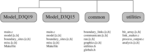
Figure 2: Program structure.

1. Model subdirectories: contain all the model-specific functions as well as main.c. These model-specific options contain three main ingredients of the code: the geometry of the lattice, the free energy that defines the type of fluid to be modeled, and the type of boundary conditions which determines the interaction with solid objects. Users can plug-in their own routines in misc.c. Once the model is defined, the only modification required to run simulations is to edit main.c to call the relevant measuring functions. At this time, the models available include the lattice geometries D3Q15, and D3Q19 (see figure 1 and reference Qian92 ; Ladd94 for their definitions), although this package has been designed to support models with subset of velocities beyond the third nearest neighbors.

2. Common subdirectory: contains all the low-level calls such as the communication layer and the parallel I/O, as well as a set of routines to provide real-time graphics during simulations. This functionality proves invaluable to gain a better understanding of the dynamics and for debugging purposes. These generic functions can be called by all models.

3. Utilities subdirectory: contains stand-alone pre- and post-processors for setting-up initial configurations and analyzing the simulation data.

The non-specificity of the common routines has been made possible by MPI’s high-level features such as derived datatypes, communicators, and user-defined operators. Indeed, these routines can be used to define series of generic and opaque objects and operators which can be accessed and manipulated without the need to know their model-specific characteristics. In effect, these routines implement a generic, generalized model, which in some ways is reminiscent of the concept of objects and methods as implemented in the object-oriented paradigm. Since the use of object-oriented programming language such as C++ or java had to be discounted on the ground of their lack of bindings for MPI-1.1 and their poor performance on HPC systems, the approach described above is in the authors’ opinion the best alternative.

The main advantage of this modular approach is the fact that the computational complexity is hidden, which allows the users to concentrate on the physical analysis of a given system rather than on implementation issues. Other advantages include code re-use, package extendibility, portability and efficiency. Ludwig achieves a high level of portability: indeed, it has been successfully installed on a variety of serial and parallel platforms (Cray T3E, T3D and J90, SGI Origin 2000, Hitachi SR-2201, Sun E-3000/HPC-3500, DEC and Sun workstations as well as a Linux PC) with no modification required.

3.4 Solid objects

Three different types of solid objects may be defined in Ludwig:

1. static solid objects, e.g. static walls and porous networks;

2. (pseudo-)moving walls, e.g. to shear the system;

3. (truly-)moving particles, e.g. freely suspended colloids.

All solid objects are implemented applying stick boundary conditions, following the bounce-back on the links (BBL) scheme proposed by Ladd Ladd94 . During propagation, the component of the distribution function that would propagate into the solid node is bounced back and ends up back at the fluid node, pointing in the opposite direction. This produces stick boundary conditions at roughly one half the distance along the link vector joining the solid and fluid nodes, ensuring that the velocity of the fluid in contact with the solid equals the velocity of the latter (see figure 3). Let us assume that a solid-fluid boundary exists between a node at $\vec{r}$ and one at $\vec{r}+\vec{c}_{i}$, where $i$ labels the relevant lattice vector. Let $i^{\prime}$ be the opposite lattice vector, so that $\vec{c}_{i}=-\vec{c}_{i^{\prime}}$. Then, at the link, there are two incoming velocity distributions after the collision; denote this time $t^{+}$. The post-collision distributions are: $f_{i}(\vec{r},t^{+})$ and $f_{i^{\prime}}(\vec{r}+\vec{c}_{i},t^{+})$. These distributions are ‘reflected’ so that:

$$f_{i}(\vec{r}+\vec{c}_{i},t+1) = f_{i^{\prime}}(\vec{r}+\vec{c}_{i},t^{+})$$ (10)

$$f_{i^{\prime}}(\vec{r},t+1) = f_{i}(\vec{r},t^{+})$$

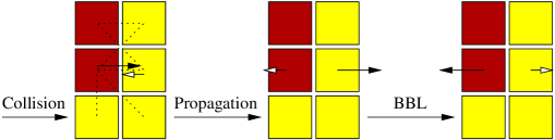
Figure 3: The bounce-back on the links (BBL) algorithm: the dark sites represent solid sites, the light sites are fluid sites; the dotted lines on the leftmost picture outlines the location of the dry links.

If the solid is moving with a velocity $\vec{u}_{b}$, the previous boundary conditions have to be modified. If the densities $f_{i}$ and order parameters $g_{i}$ are allowed to ‘leak’ across the boundary links, then the velocity at the link can be matched to the velocity of the wall Ladd94 . In the case of a binary mixture, generalizing the results of Ladd Ladd94 , the basic BBL scheme is modified as follows:

$$f_{i}(\vec{r}+\vec{c}_{i},t+1) = f_{i^{\prime}}(\vec{r}+\vec{c}_{i},t^{+})+6t^{i}\rho\vec{u}_{b}\cdot\vec{c}_{i}$$ (11)

$$f_{i^{\prime}}(\vec{r},t+1) = f_{i}(\vec{r},t^{+})-6t^{i}\rho\vec{u}_{b}\cdot\vec{c}_{i}$$

$$g_{i}(\vec{r}+\vec{c}_{i},t+1) = g_{i^{\prime}}(\vec{r}+\vec{c}_{i},t^{+})+6t^{i}\phi\vec{u}_{b}\cdot\vec{c}_{i}$$

$$g_{i^{\prime}}(\vec{r},t+1) = g_{i}(\vec{r},t^{+})-6t^{i}\phi\vec{u}_{b}\cdot\vec{c}_{i}$$

where the quantities $t^{i}$ are geometric factors related to the weights of the different subsets of velocities $\vec{c}_{i}$, and are fixed when imposing the appropriate equilibrium distribution functions for $f_{i}$ and $g_{i}$. Note that the BBL rules given above require careful implementation if they are properly to account for the effect on the composition variable $\phi$ of motion in a direction normal to the solid-fluid boundary. This boundary condition allows us to have a solid wall moving in any direction in contact with the fluid Warren .

The velocity of the solid particles can be fixed beforehand. In this case, one can use such moving objects e.g. to apply a shear flow through parallel plates at the boundaries of a sample, or to study aspects of colloid hydrodynamics such as the steady-state sedimentation of an ordered array of colloidal spheres with a prescribed distribution. Alternatively, if the velocities of the solid particles are updated, one can for example simulate the dynamics of colloidal suspensions Ladd94 .

3.5 Boundary conditions

Although periodic boundary conditions are applied to the model by default, these can be modified by explicitly adding solid surfaces at the boundaries. In the previous subsection we have shown how to add them ensuring stick boundary conditions. This is enough for a mono-component simple fluid. However, for complex fluids it is also in general necessary to specify the behavior of additional fields at solid boundaries, whether these are at the edges of the system or internal boundaries between fluid and solid phases.

For example, in the case of a binary mixture it may be desirable to specify the wetting properties of a solid surface, i.e. its preference for one of the two components. In order to deal with these situations, we have developed in Ludwig a more generic way of characterizing a solid interface. We have considered three different kinds of sites on the lattice: solid, fluid and boundary sites (the latter are fluid sites with at least one neighboring solid site). Accordingly, the links are then classified as wet or dry links depending on whether they join fluid sites or solid to fluid sites, respectively. Then, in order to implement the appropriate thermodynamic boundary conditions at the solid-fluid interfaces (which we discuss in detail in the next section), the values of $f_{i}$ and $g_{i}$ corresponding to the boundary sites and dry links are stored in two separate lists, different from the basic vectors which store $f_{i}$ and $g_{i}$ for all sites. Note that additional information also needs to be stored for the boundary links and boundary sites. The structure defined to store this information is called bc_link. In addition to the location and orientation of the links, it also contains the force applied on the node and its velocity, in case it is needed.

typedef struct bc_link BC_Link;
struct bc_link{
	Int i,j,		/* i and j are the indices of the two nodes
			By convention, i is the (local) solid node,
			j is the fluid node */
		index,	/* index is the velocity that links the two nodes */
		dup;	/* TRUE when a duplicate link */
	Float frc,		/* Force on the node at (r+0.5*c,t+0.5) in direction c */
		v;	/* Velocity component of link */
	BS_Site *site;		/* Only relevant to wetting: pointer to the site with the
			value of the concentration at the middle of the link */
	BC_Link *next;		/* Store these in a singly linked list */
};

Note that all members of this list have a pointer *site to the corresponding element of the boundary site list. Links that have their ends on different PE domains (i.e. partly in the halo region) need to be duplicated on both PEs. The structure member dup is therefore required to avoid multiple counting when carrying out summations over all links. This structure is enough to implement the BBL described in the previous subsection.

Similarly, boundary sites are stored in a structure of type bs_site, which includes information mostly required for the implementation of the thermodynamic boundary conditions (wetting effects). These include the free energy parameters of the neighboring wall, the fluid or solid nature of the NGRAD neighboring sites (i.e. a binary map of dry or wet links to these sites), as well as the actual gradient on the link which value is required by the BBL algorithm described in section 3.4. The extended set defined by NGRAD includes all vectors to nearest neighbors, next nearest neighbors, next-but-one nearest neighbors, and the null vector (thus for a 3-D cubic lattice (D3Q15), NGRAD = 27). This extended set of neighbors has been introduced to improve the representation of the order-parameter gradients close to the wall.

typedef struct bs_site BS_Site;
struct bs_site{
	Int ind;	/* (Global) index of site */
	UInt wet;	/* Binary number specifying ‘wet’ and ‘dry’ links */
	Float C,H;	/* Value of C and H in surface free energy */
	Float phi[NGRAD];	/* Gradients on the link (along NGRAD vectors) */
	BS_Site *next;	/* Store these in a singly linked list */
};

Note that the actual implementation of the BBL is undertaken by applying equation 11 to all the (dry) links in the linked list BC_Link. Whilst the $f_{i}$ and $g_{i}$ can be accessed directly using their array index, the link velocities $\vec{u}_{b}$ and composition variable $\phi$ need to be retrieved from the structure itself as BC_Link$\rightarrow$v and BC_Link$\rightarrow$site$\rightarrow$phi[] respectively.

Another aspect worth pointing out is that both structures are defined in different directories (see figure 2). Indeed, although the boundary_sites functions are intrinsically model-specific because they depend on the velocity sets and free energy parameters, the boundary_links routines on the other hand are completely independent from the model used.

3.6 Moving particles

The implementation of static solid objects and moving walls in parallel is simple. Indeed, since these objects do not move across PE domains during the course of a simulation, one needs only to build the two linked lists BC_Link and BS_Site once, and independently for each node.

The case of moving solid particles is more complicated and deserves further discussion. Although non-spherical objects can be described vanderhoef , we restrict the discussion to spherical ones for simplicity’s sake. In this case they are defined by four parameter; their radius $R$, the position of their center of mass ${\bf r}_{CM}$ and their linear and angular velocities, ${\bf u}$ and ${\bf\omega}$. Note that although ${\bf r}_{CM}$ moves continuously, the surface of the particle is discretized since it is defined by the lattice links which would cross the surface. Each particle can therefore be defined as follows:

typedef struct colloid Colloid;
struct colloid{
	Int index;		/* Global index of colloid (0..N_colloid-1) */
	FVector r,		/* Position of the center of mass */
		v, w,	/* Linear and angular velocity of the center of mass */
		T, F;	/* Torque and force */
	Float R;		/* Radius */
	Int	*pe;	/* List of PE domains span by this colloid */
	Int	local;	/* TRUE for local PE, FALSE otherwise */
	COLL_Link *lnk;		/* Pointer to list of links (surface) */
	Colloid *next;		/* Store these in a singly linked list */
};

where the list of links required to describe the surface of each colloid is stored in a separate linked list of type coll_link:

typedef struct coll_link COLL_Link;
struct coll_link{
	Int i,j,		/* i and j are the indices of the two nodes
			By convention, i is the inner node,
			j is the outer node */
		index,	/* index is the velocity that links the two nodes */
		dup,	/* TRUE when a duplicate link
			(set when crossing different PE domains) */
		local;	/* TRUE for local PE, FALSE otherwise */
	Float dist;		/* Distance from middle of link to center of mass */
	COLL_Link *next;		/* Store these in a singly linked list */
};

In order to update the velocities of the particle at each time step it is necessary to know the force and torque exerted by the fluid on the particle. These are computed from the change in momentum of the fluid at each link after it has bounced back. The motion of the colloid evolves as in a molecular dynamics step. The discretization of the particle surface onto the lattice links implies its radius is not strictly constant. It is therefore necessary to keep the actual distance between the center of the link and the center of mass of the particle for each link as a separate variable dist to compute the torque.

The complete information about any given colloid is replicated on all the PEs which have their local domain intersected by it (list stored in colloid.pe). The variable coll_link.local tells which (non-local) links must be skipped during the BBL, which is implemented by applying equation 11 just like for any other solid objects. Contributions to the torque from each link will be summed locally and then across PEs.

The radius of the colloids must be larger than the lattice spacing, and its actual value will depend on the volume fractions of solid particles considered. Up to around $40\%$ in volume fraction, a small value of the radius, e.g. 2.5 lattice spacings, is sufficient to get accurate results hagen . At higher volume fractions, larger radii should be considered. This will eventually, at very high packing fractions, limit the performance of the LB code, as progressively larger system sizes will be needed. Similar limitations will apply when dealing with polydisperse suspensions, or motion of non-spherical objects. A more complete discussion of the implementation, optimization, and application of moving solid particles will be published elsewhere.

3.7 Wetting

As pointed out already, for a two component fluid, the interaction with a solid wall should allow a difference in interaction between the two components and the wall even when the fluids are symmetric in all other respects. It can be energetically favorable for one of the two components to be in contact with the solid surface, in which case, in static equilibrium the fluid-fluid interface is not perpendicular to the wall. The equilibrium angle $\theta$ is called the contact angle and is determined, via the Young equation Rowlinson

$$\gamma_{sl}^{+}-\gamma_{sl}^{-}-\gamma_{ll}\cos(\theta)=0$$ (12)

where $\gamma_{sl}^{+(-)}$ is the solid/fluid surface tension for the bulk phase with positive (negative) order parameter, and $\gamma_{ll}$ is the fluid-fluid surface tension.

The resulting wetting phenomena are known to play a major part in the behavior of complex fluids next to (or including) solid objects, but their implementation in simulations still remains in its infancy Grubert ; Yeomans95 . In particular, it is important to make sure that the observed wetting behavior is consistent with the thermodynamic requirement of Young’s equation in equilibrium. We have therefore devised a novel predictor-corrector scheme to ensure an accurate implementation of controlled wetting effects at the solid-fluids interface in three dimensions. Recalling that Ludwig uses a symmetric $\phi^{4}$ model free energy (see equation 2), a simple way to account for wetting properties is to associate with the solid surfaces an additional surface free energy density $f_{s}(\phi_{s})$, where $\phi_{s}$ is the value of the compositional order parameter in contact with the wall. According to Cahn theory Cahn , the equilibrium order parameter profile corresponds to that which minimizes the free energy functional $F=F_{bulk}[\phi]+\int f_{s}(\phi_{s})dS$ where $F_{bulk}$ obeys equation 2 and the integral is over the solid surface. The two solid-fluid interfacial tensions are found by minimizing this expression near a flat solid-fluid interface to find the equilibrium free energy $F$, subtracting the contribution $\int F_{bulk}[\phi^{*}]\,d\mathbf{r}$ of the same volume of bulk fluid, and dividing by the interfacial area. The functional minimization also gives the composition profile near the wall, and the boundary condition satisfied at the solid surface, which is

$$\frac{d{f}_{s}}{d\phi_{s}}=\kappa\left|\nabla\phi\cdot{\vec{n}}\right|$$ (13)

where $\vec{n}$ is normal to the wall.

In general, ${f}_{s}$ is a function of the local order parameter. The classical work on wetting has shown that a functional relation of the form

$${f}_{s}=\frac{C}{2}\phi_{s}^{2}+H\phi_{s}$$ (14)

is enough to reproduce the various different wetting scenarios Cahn . By tuning the parameters $C$ and $H$, we modify the properties of the surface in a thermodynamically controlled manner Cahn , so that the fluid-solid interfacial tensions can be tuned at will. Since we are dealing with a symmetric mixture, if $H=0$ the two phases will have neutral wetting and show a local variation in composition near the wall ($\phi_{s}-\phi^{*}$) of the same magnitude. Nonzero $H$ allows then for an asymmetry in the surface value of the order parameter for the two coexisting phases and a contact angle different from $90$ degrees.

The main difficulty to implement the general boundary condition, equation 14, is that it depends on the value of the order parameter at the surface, $\phi_{s}$, which is itself a dynamical variable. Moreover, due to BBL, the solid surface lies between the sites thus making the calculation of $\nabla\phi$ and $\nabla^{2}\phi$ by finite difference from neighboring sites using equations 8 and 9 impossible. To circumvent this, we use a predictor-corrector scheme to estimate the gradient at the solid wall as follows (see figure 4):

1. determine which sites are next to a wall (boundary sites), and hence which links cross the wall (i.e.  dry links);

2. estimate $\nabla\phi$ using finite differences on all wet links;

3. from this estimate of $\nabla\phi$, extrapolate to halfway along the dry links, and calculate $\phi_{s}$; using $\phi_{s}$ on the dry links, calculate $\nabla\phi\cdot{\vec{n}}$ on these links;

4. calculate $\nabla\phi$ and $\nabla^{2}\phi$ for the boundary sites using all the gradients estimated on the links.

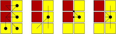
Figure 4: The wetting algorithm.

This scheme gives good quantitative results of the wetting angles in accordance with thermodynamic predictions. Results from case studies, both for a droplet and for planar interfaces are discussed in section 4.

3.8 Computational issues

Production runs on the phase separation kinetics of binary fluid mixtures have been carried out on the Cray T3D and the Hitachi SR-2201 at EPCC, and on the Cray T3E-1200 at CSAR Kendon00 ; Kendon99 ; Cates99 . In addition to these distributed memory systems, we also investigated the performance of the code on shared-memory platforms such as the SUN HPC-3500 at EPCC.

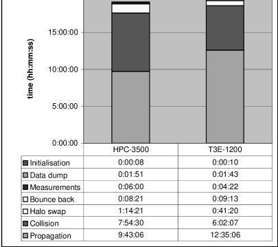
Figure 5: Time spent in each function (average clock time per processor). These timings have been obtained for the simulation of spinodal decomposition under shear. The system was specified as follows: D3Q15 model on a cubic lattice of size $L=180$ distributed on 8 PEs for 12,000 steps. The shear has been applied through fixed walls at constant velocity, thus requiring a total of $2.7\times 10^{6}$ BBLs per step. The order parameter and velocity fields were saved 60 times and the full configuration only once, thus representing a combined output of 17Gb for the simulation. The darkest color at the top of the bar chart represents the remaining stages of the simulation (i.e. initialization, BBL, measurements, and I/O).

The profile information reproduced in figure 5 provides us with an interesting insight on the critical sections of the code. Firstly, one notices that over 90% of the simulation time is spent in the collision and propagation stages which are both intrinsically serial and well load-balanced for most problems. The raw performance (excluding all I/O and measurements) varies from $1.04\times 10^{6}$ to $1.10\times 10^{6}$ gridpoint-updates per second for the Cray T3E and SUN HPC-3500 respectively. Details of the timing information for the various stages of the simulation of spinodal decomposition under shear is given in figure 5. Note that the halo swap and BBL only account for 4-7%. A comparison of the profiles obtained on the Sun HPC-3500 and Cray T3E-1200 also shows up that the critical parts of the code are highly system dependent. As expected, the increased clock speed of the T3E-1200 (600MHz compared to only 400MHz on the HPC-3500) benefits the collision stage which is a highly-localized algorithm with basic arithmetic operators (add/multiply). This routine has been highly optimized and makes a good use of the T3E memory hierarchy. On the other hand, the memory-to-memory copies performed in the propagation stage do not benefit from this increase in clock speed as much. Indeed, the HPC-3500 significantly outperforms its rival by over 23% even though the algorithm for the propagation had been tuned for the T3E by rearranging loops to make an efficient use of its streams (see CRI-streams for further information about stream optimization). Particular attention should also be paid to finding the optimal ordering for the velocity set $\{c_{i}\}$. It is important to order the velocity set such that they correspond, as much as possible, to sequential positions in memory for the distribution functions. The first production platform for this package was the Cray T3D which, due to its lack of second-level cache, was particularly sensitive to data locality. The arrangement reproduced in table 1 proved to be the most effective to preserve data locality with a performance increase of over 20% on the T3D (compared to an unoptimized sequence) for the combined collision and propagation stages. Note that some orderings can speed-up one of these stages alone and be detrimental to the second one. The gain in performance resulting from data locality is not as significant on systems with second-level cache though. The ‘best’ ordering of the velocity vectors is therefore often system-specific.

Table 1: ‘Optimal’ velocity set for the Cray T3D

c(0) =( 0, 0, 0)	c(1) =( 1,-1,-1)	c(2) =( 1,-1, 1)
c(3) =( 1, 1,-1)	c(4) =( 1, 1, 1)	c(5) =( 0, 1, 0)
c(6) =( 1, 0, 0)	c(7) =( 0, 0, 1)	c(8) =(-1, 0, 0)
c(9) =( 0,-1, 0)	c(10)=( 0, 0,-1)	c(11)=(-1,-1,-1)
c(12)=(-1,-1, 1)	c(13)=(-1, 1,-1)	c(14)=(-1, 1, 1)

As shown in figure 6, Ludwig also demonstrates near-linear scaling from 16 up to 512 processors. However, the overall cost of the I/O can become a major bottleneck for the unwary (e.g. a $512^{3}$ system will generate in excess of 31Gb per configuration dump). The I/O has been optimized by performing parallel I/O. The pool of PEs is split into $N$ groups of $p$ processors, thus providing $N$ concurrent I/O streams (typically, $N=8$). Each group has a root PE which will perform all I/O operations. The remaining $(p-1)$ PEs send their data in turn to the I/O PEs which pack these data and write them to disk. This approach usually offers high bandwidth without having to use platform specific calls such as disk striping.

Figure 6: Scale-up: scaling figures have been normalized with respect to the time taken for the lowest number of processors, $N_{PE}=16$. Details of the simulation are similar to that given in figure 5 with the exception of the system size which has been increased to $L=232$. The only quantity measured during this benchmark is the order parameter field, $\phi_{i}$ which was measured and saved to disk every 50 iterations. Speed-up data have been included for simulations with and without the I/O (note that in both cases, the time taken for dumping full re-start configurations was not included). The I/O consists in 240 data dumps of 191 Mb written to disks through eight parallel output streams.

Note that MPI2-IO had initially to be discounted on the ground of portability and performance. We conclude this discussion by deploring the lack of a full support for MPI-2 single-sided communications on some platforms. Indeed, this functionality proves invaluable for the implementation of the Lees-Edwards boundary conditions and moving particles.

4 Results for wetting behavior

Ludwig has already been used to study a number of problems for binary fluid mixtures of current interest:

1. establishment of the role of inertia in late-stage coarsening Kendon00 ; Kendon99 ;

2. study of the effect of an applied shear flow on the coarsening process Cates99 ;

3. persistence exponents in a symmetric binary fluid mixture Kendon00b .

These results have been published elsewhere and will not be discussed further here. A number of validation exercises relating to binary mixtures are also described in Kendon00 . Here we focus on discussing new validation results obtained using the novel predictor-corrector scheme for the thermodynamically consistent simulation of wetting phenomena, as presented earlier.

We present results for two types of tests for the properties of binary fluids near a solid wall. First, we verify that the modified bounce-back procedure, equation 11, gives the expected balance both for the momentum and for the order parameter. Second, we check the numerical accuracy of the modified boundary condition that accounts for the wetting properties of the wall, equation 14, as implemented through the predictor-corrector step.

To test the validity of the modified bounce-back rule for the order parameter field, we have looked at the motion of a pair of planar interfaces perpendicular to two parallel planar solid walls when the whole system is moving at a constant velocity parallel to the walls. The initial condition corresponds to a stripe of one equilibrium fluid ($\phi=\phi^{*}$), oriented perpendicular to the walls, surrounded by a region of the other fluid ($\phi=-\phi^{*}$), with periodic boundary conditions. Due to Galilean invariance, the profile should remain undistorted and move at the same velocity as it is moving with initially, but with LB this is not guaranteed a priori and has to be validated. We have considered both the case of neutral wetting and the asymmetric case where $H$ is nonzero.

Figure 7: Leading interface of a binary mixture fluid. Initially a stripe perpendicular to two parallel moving walls is set up. The two walls move at the same speed, 0.005 in lattice units, towards the right. The two interfaces that characterize the stripes are recorded every 1000 time steps (which corresponds to a theoretical displacement of the two interfaces of 5 lattice units), and the leading one is shown. The wall is neutral, which implies that no phase is favored at the wall, and therefore the stripe wants to remain perpendicular. We show the interfaces for the bounce-back described in equation 10 (open circles), and also for a bounce-back of the order parameter field in which the advection induced by the moving walls is neglected (filled diamonds).

For neutral surfaces, we show in figure 7 the leading interfacial profiles at different times, both for the bounce-back rules described in equation 10, and for an improperly formulated bounce-back of the order parameter that does not take into account the motion of the wall. (The latter is equivalent to assuming $t^{p}=0$ only in the equations describing the bounce-back of the order parameter distribution function.) As can be seen, although the profile is advected due to the existence of a net momentum at the wall, if the bounce-back is not done in the frame of reference of the moving wall (leading to equation 11) the fluid-fluid interface has a spurious curvature and it moves more slowly than it should. From the rectilinear shape of both the leading (shown in figure 7) and trailing interfaces of the rectangular strip, we have found that Galilean invariance is in fact well satisfied with equation 11. Figure 7 corresponds to a situation of high viscosity and low diffusion ($\eta=10,\tilde{M}=0.01$) but the same features have been observed for a number of different physical parameters. The magnitudes of the errors made by using the inappropriate bounce-back, in this geometry, are found to decrease upon increasing the mobility, probably because a large mobility allows a faster relaxation to the imposed velocity profile in the interfacial region (especially near the contact with the walls).

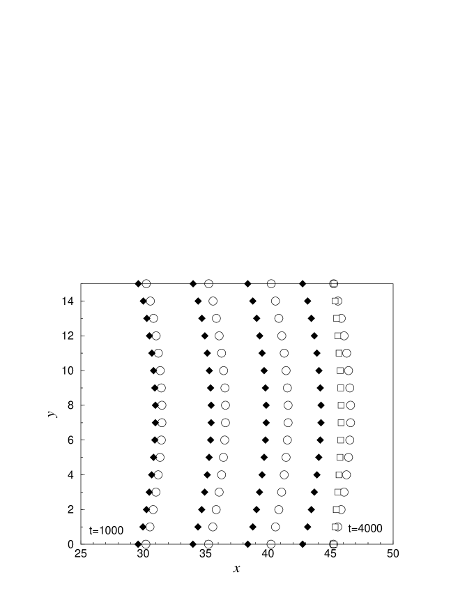
Figure 8: Leading interface of a moving binary mixture fluid stripe. Same geometry and parameters as in figure 7. The walls wet partially, and therefore the stripe relaxes from its initial configuration to a bent interface. We show the interfaces for the bounce-back described in equation 10 (open circles), and also for a bounce-back of the order parameter field in which the advection induced by the moving walls is neglected (filled diamonds). In open squares we show the trailing interface at time 4000 to show the magnitude of the deviations with respect to Galilean invariance (see text).

In figure 8 we show the same configuration as described in the previous paragraph, but for the case in which the solid surface partially wets one of the two phases, so that $H$ is nonzero and $\theta=60$ rather than 90 degrees. In this case the profile should relax from the initial perpendicular stripe to a curved interface. Again, the use of inappropriate bounce-back for the order parameter leads to a slower motion of the interface, and a significant distortion away from the equilibrium interfacial shape. In order to test Galilean invariance here, for the final interface ($t=4000$ timesteps) we have compared the leading and trailing edge of the stripe. There is a slight deviation in this case, implying that the asymmetry entering via $H$ couples through to the overall fluid motion relative to the underlying lattice, which (by Galilean invariance) it should not. However, the resulting violation is very small, and the interfacial deviations do not grow beyond one lattice spacing.

We have also verified that if the velocity of the walls is perpendicular to their own plane, then an order parameter profile, initially in equilibrium, remains stationary. This confirms that the chosen boundary conditions can account for generically moving interfaces for the case of a binary mixture.

Finally, for stationary walls, we have computed the contact angles for the simplest asymmetric case in which $C=0$ (see equation 14). In this situation the order parameter at the wall will deviate by the same magnitude, but with opposite sign, in the two bulk phases. For this choice (with $A=-B$) the contact angle, $\theta$, is predicted to depend on the parameter $h=H\sqrt{1/(\kappa B)}$ according to

$$cos(\theta)=\frac{1}{2}\left[-(1-h)^{3/2}+(1+h)^{3/2}\right]$$ (15)

We have considered a geometry in which the two solid walls have the same wetting properties. We start, as in the previous case, with an initial stripe perpendicular to the walls, defining two regions with opposite equilibrium values for the order parameter. The equilibrium profile for the interface then corresponds to a cylindrical cap. By fitting the cylindrical cap it is possible to get a numerical value for the contact angle. In figure 9 we show the measured contact angles as a function of $h$ for different interfacial widths $\xi_{0}=(\kappa/2A)^{1/2}$, and compare these with the above theoretical prediction. (Note that, by maintaining fixed $A/B$ have kept constant the values $\pm\phi^{*}$ of the equilibrium order parameters in the two coexisting phases.) As can be seen, the agreement between the theoretical prediction and the measured contact angle is quantitative.

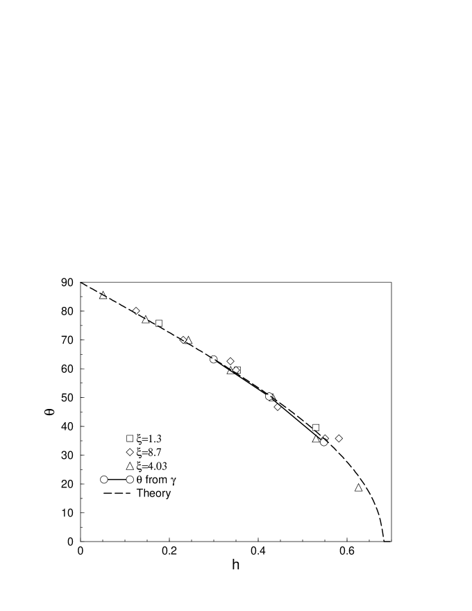
Figure 9: Contact angles for the equilibrium profile of an interface in contact with a wetting surface. $\xi=\sqrt{\kappa/B}$ is the liquid/liquid interfacial width expressed in lattice units.

The parameters that characterize the binary mixture have been chosen to ensure fairly wide fluid-fluid interfaces. (In fact, the smallest interfacial width, $\xi_{0}=1.3$, is at least twice as large as that used previously in production runs for binary fluid demixing Kendon00 .) For narrower interfaces than this, the contact angles can differ significantly from the predictions due to anisotropies induced by the lattice, whose effects were studied (for fluid-fluid interfaces only) in Kendon00 . This effect should be more relevant for small contact angles. Indeed, when a narrow fluid-fluid interface has a glancing incidence with the solid wall, the discrete separation of lattice planes will lead to significant errors in the estimation of the order parameter gradients; the direction of these not only determines the surface normal of the fluid-fluid interface, and hence the contact angle, but is crucial to an accurate estimate of the free energies near the contact line. However, except perhaps for small contact angles, there is not much accuracy gained from choosing $\xi_{0}$ larger than $1.3$.

Because of the finite width of the interfaces, one has to be careful to measure the contact angle by extrapolation from regions of fluid-fluid interface that are more than about $\xi_{0}$ from the wall. To check that we did this correctly, we have also numerically and analytically computed the three interfacial tensions directly by the method outlined in section 3.7. From the values of the surface tensions obtained, it is the possible to get values for the contact angles, through Young’s law, equation 12. As expected, the values agree with the theoretical predictions and the contact angles measured from the profiles (figure 9).

5 Conclusions

We have described a versatile parallel lattice Boltzmann code for the simulation of complex fluids. The objective has been to develop a piece of code that allows to study the hydrodynamics of a broad class of multicomponent and complex fluids, focusing initially on binary fluid mixtures with or without solid surfaces present. It combines a parallelization strategy, making it suitable to exploit the capabilities of supercomputers, with a modular structure, which allows its use without the need to know its computational details, and with the possibility of focusing on the physical analysis of the results. This strategy has led to a code that is in principle adaptable to several different uses within the academic collaboration involved Kendon00 ; Kendon99 ; Cates99 .

We have discussed how to introduce generic fluid-solid boundary conditions, and discussed which structures were developed to combine the requirements of specific physical features with the generic structure of the code. The performance of the code in different computers shows its portability, and it scales up efficiently on parallel computers.

We have implemented generic boundary conditions for a binary mixture in contact with moving solid interfaces. We have shown how one recovers appropriate behavior of the momentum and the fluid order parameter so long as the bounce-back rule, in the moving frame of the wall, is performed with the distribution function that characterizes the order parameter as well as that for momentum (equation 11). A mesoscopic boundary condition that accounts for the wetting properties of a binary mixture near a solid surface has been described. It has been shown how to deal appropriately with the gradients of the order parameter at the wall, and with the role of the finite interfacial width when analyzing the results. The values obtained for the contact angle agree with the predictions of the model simulated, showing the absence of lattice artifacts, at least for contact angles larger than about 20 degrees. These results are, however, for planar solid interfaces oriented along a lattice direction. We have not checked in detail the dependence of the contact angle on the orientation of the solid surface, and it may require further work on the discretization of order parameter derivatives before this isotropy can be relied upon. Analogously to the problem of small wetting angles mentioned above, the problem may prove most acute for low-angle inclination of the solid surface, where the naive discretization of the solid phase leads to a series of well-separated steps in the wall position.

Current and planned work with Ludwig includes the hydrodynamic simulation of multicomponent fluid flow in a porous networks with controlled wetting; implementation of Lees-Edwards (sliding periodic) boundary conditions; large-scale simulations of binary fluids under shear, and the improvement of the gradients to make the thermodynamics of this model more fully independent of the underlying symmetries of the lattice. Longer term plans include studying colloid hydrodynamics and extending Ludwig to study amphiphilic systems under shear (see Jury99b for an example of this studied by DPD).

The authors would like to acknowledge Michael Cates, Simon Jury, Alexander Wagner, Patrick Warren, and Julia Yeomans for valuable discussions. They thank Michael Cates for assistance with the manuscript. This work has been funded in part under the Maxwell Institute’s project on ‘Fluid Flow in Soft and Porous Matter’ and the EPSRC E7 Grand Challenge and GR/M56234.

References

- (1) C. Denniston, E. Orlandini and J. Yeomans, cond-matt/9904033.
- (2) F.J. Higuera, S. Succi and R. Benzi, Europhys. Lett. 9 (1989) 345.
- (3) Y.H. Qian, D. D’Humières and P. Lallemand, Europhys. Lett. 17 (1992) 479.
- (4) A.J.C. Ladd, J. Fluid Mech. 271 (1994) 285.
- (5) S. Wolfram, J. Stat. Phys. 45 (1986) 471.
- (6) M.R. Swift, E. Orlandini, W.R. Osborn and J. Yeomans, Phys. Rev. E 54 (1996) 5041.
- (7) D. Grubert and J.M. Yeomans, Comp. Phys. Commun. 121-122 (1999) 236.
- (8) V.M. Kendon, M.E. Cates, J.-C. Desplat, I. Pagonabarraga and P. Bladon, in preparation.
- (9) V.M. Kendon, J.-C. Desplat, P. Bladon and M.E. Cates, Phys. Rev. Lett. 83 (1999) 576.
- (10) R.D. Groot and P.B. Warren, J. Chem. Phys. 107 (1997) 4423.
- (11) I. Pagonabarraga and D. Frenkel, preprint.
- (12) I. Foster, Designing and building parallel programs, Addison Wesley Publishing Company, 1995.
- (13) We are grateful to Dr. P.B. Warren for a discussion on this point.
- (14) C.P. Lowe, D. Frenkel and A.J. Masters, J. Chem. Phys. 103, 1582 (1995).
- (15) M.H.J. Hagen, D. Frenkel and C.P. Lowe, Physica A 272, 376 (1999).
- (16) J. Rowlinson and B. Widom, Molecular theory of capilarity, Clarendon Press, Oxford 1982.
- (17) M.R. Swift, W.R. Osborn and J. Yeomans, Phys. Rev. Lett. 75 (1995) 830.
- (18) J. Cahn, J. Chem. Phys. 66 (1977) 3667.
- (19) Cray Research Inc., Cray T3E programming with coherent memory streams v1.2, (1996).
- (20) M.E. Cates, V.M. Kendon, P. Bladon and J.-C. Desplat, Faraday Discussions 112 (1999) 1.
- (21) V. Kendon, M.E. Cates and J.-C. Desplat, Phys. Rev. E 61 (2000) 4029.
- (22) S. Jury, P. Bladon, M.E. Cates, S. Krishna, M. Hagen, N. Ruddock and P. Warren, Phys. Chem. Chem. Phys. 1 (1999) 2051.