Hopping in Disordered Media:
A Model Glass Former
and
A Hopping Model

1.1 Abstract

Two models involving particles moving by “hopping” in disordered media are investigated:

A model glass-forming liquid is investigated by molecular dynamics under (pseudo-) equilibrium conditions. “Standard” results such as mean square displacements, intermediate scattering functions, etc. are reported. At low temperatures hopping is present in the system as indicated by a secondary peak in the distribution of particle displacements during a time interval $t$. The dynamics of the model is analyzed in terms of its potential energy landscape (potential energy as function of the $3N$ particle coordinates), and we present direct numerical evidence for a 30 years old picture of the dynamics at sufficiently low temperatures. Transitions between local potential energy minima in configuration space are found to involve particles moving in a cooperative string-like manner.

In the symmetric hopping model particles are moving on a lattice by doing thermally activated hopping over energy barriers connecting nearest neighbor sites. This model is analyzed in the extreme disorder limit (i.e. low temperatures) using the Velocity Auto Correlation (VAC) method. The VAC method is developed in this thesis and has the advantage over previous methods, that it can calculate a diffusive regime in finite samples using periodic boundary conditions. Numerical results using the VAC method are compared to three analytical approximations, including the Diffusion Cluster Approximation (DCA), which is found to give excellent agrement with the numerical results.

Contents

1. 1.1 Abstract
2. 2 Introduction
   1. 2.1 Outline
   2. 2.2 Acknowledgments
   3. 2.3 Papers
3. 3 A Model Glass-former
   1. 3.1 Model and Method
   2. 3.2 Static Results
   3. 3.3 Mean Square Displacement
   4. 3.4 The van Hove Correlation Function
   5. 3.5 The Intermediate Scattering Function
   6. 3.6 Time Scales
   7. 3.7 Finite Size Effects
   8. 3.8 Conclusions
4. 4 Inherent Dynamics
   1. 4.1 The Potential Energy Landscape
   2. 4.2 The Inherent Dynamics
   3. 4.3 Paper III
   4. 4.4 Paper II
   5. 4.5 Transitions between inherent structures
   6. 4.6 Conclusion
5. 5 The Symmetric Hopping Model
   1. 5.1 The Symmetric Hopping Model
   2. 5.2 The Master Equation
   3. 5.3 Analytical approximations
   4. 5.4 The ACMA Method
   5. 5.5 The Velocity Auto Correlation (VAC) method
   6. 5.6 Numerical results, $D(s)$
   7. 5.7 Numerical Results, $D(\omega)$
   8. 5.8 VAC vs. ACMA
   9. 5.9 Conclusions
6. A Numbering scheme for VAC method

Chapter 2 Introduction

This Ph.D. thesis deals with two models characterized by particles moving by “hopping” in disordered media. The first model is a simple model glass-former, investigated here by computer simulations using molecular dynamics [1]. Glass forming liquids are liquids that upon cooling falls out of equilibrium and form a glass, see figure 2.1. For general reviews on glass-forming liquids see [2, 3, 4, 5, 6]. For reviews on computer simulations of glass-forming liquids see [7, 8, 9, 10, 11].

Figure 2.1: Schematic overview of the behavior of glass-forming liquids. Upon cooling crystallization is avoided and the liquid becomes “supercooled”, which is a (pseudo-) equilibrium state (the crystal being the real equilibrium state). Upon further cooling the liquid falls out of equilibrium and undergoes a glass-transition at the temperature $T_{g}$. $T_{g}$ depends on cooling rate; glass II is obtained by a lower cooling rate than glass I.

The normal liquid behavior is to crystallize upon cooling below the melting temperature, $T_{L}$. In a large class of liquids the crystallization can be avoided (e.g. by fast cooling) and the liquid becomes “supercooled”. A supercooled liquid is in a pseudo-equilibrium state; The crystal is the real equilibrium state, but the supercooled state is typically stable on very long time scales. The supercooled state is characterized by relaxation times increasing strongly with decreasing temperature. If cooled with a constant cooling rate this means that the liquid at some temperature falls out of equilibrium and undergoes a glass-transition and forms a glass, which is a disordered solid. The glass-transition temperature, $T_{g}$, depends on the cooling rate; a lower cooling rate results in a lower glass transition temperature. By convention the “laboratory” glass transition is taken to be where the relaxation time $\tau$ is on the order of 100 sec (i.e. the “typical” time scale in the laboratory).

Binary systems with particles differing about 20% in diameter have been found to be good candidates for simple models of glass-forming liquids in computer simulations [12, 13, 14, 9, 8, 15, 16, 17, 18]. At sufficiently low temperatures particles in these systems are found to move by “hopping”, i.e. they are localized for a period of time, and then move more or less directly to another position, where they again become localized [12, 13, 14, 9, 8, 15, 16]. Since hopping of some form is expected to play a increasingly dominant role as temperature is lowered [19, 20], systems exhibiting hopping at temperatures which can be reached under equilibrium conditions in computer simulations are of special interest. In this thesis we investigate the dynamics of a binary Lennard-Jones liquid, which has earlier been shown to exhibit hopping [15]. This is done under (pseudo-) equilibrium conditions, i.e. above the glass transition temperature.

The model glass-former investigated in this thesis is not a model of any particular liquid existing in the laboratory (or the real world for that matter). Like most models glass formers studied in computer simulations, it should be thought of as a (very) simple model exhibiting some of the complex behavior found in real glass forming liquids. The reason why it is interesting to investigate such a simple model is two-fold: I) The glass-transition is found to occur in liquids that are chemically very different, but the related phenomenology is found to be strikingly similar. Since liquids with different chemical details behave in a similar way, it makes sense to study simple models ignoring the chemical details, in an attempt to understand the fundamental mechanisms. II) Most theories for glass-forming liquids also treat these in a highly simplified manner, ignoring the chemical details (for the same reasons given above). Consequently computer simulations makes it possible to test these theories on their own terms, i.e. without any additional approximations. One particular example of this is the Mode Coupling Theory (MCT) [21, 22]. When doing computer simulations of glass forming liquids it is rather natural to compare the results with the predictions of the MCT since these are plenty and detailed, and MCT deals with the temperature range accessible (at the present) to computer simulations under equilibrium conditions. It is not a goal in it self to test MCT in the present thesis, but some of the results are compared to the predictions of the MCT.

The second model investigated in the present thesis is a so-called “hopping-model”, where the hopping behavior of particles is “built in”; In the symmetric hopping model [23, 24, 25, 26, 27, 28] particles are moving on a lattice by doing thermally activated hopping over random energy barriers. This model is found to have interesting universal features in the extreme disorder limit, i.e. when the temperature goes to zero. The symmetric hopping model has earlier been treated as a model for frequency dependent conduction in glasses [23, 25], with particles representing non-interacting charge carriers (ions or electrons). In that context the universality manifests itself as follows: At low temperatures the shape of the conduction vs. frequency curve becomes independent of temperature, which is also what is found in experiments (see eg. [29, 30, 31]). In the present thesis the symmetric hopping model is treated in the slightly more general context of diffusion in disordered media.

2.1 Outline

This thesis consists of 3 main chapters:

In chapter 3 we report results from the simulations of the model glass-former mentioned above, with emphasis on the dynamics. In this chapter “standard” results are reported, i.e. the measures commonly used to describe (glass-forming) liquids. All of the features found for this particular model has been reported earlier for other models, and this chapter thus constitutes a “review” of the behavior of model glass-formers, illustrating the similarities in the behavior of these.

In chapter 4 the dynamics of the model glass-former described in chapter 3 is investigated in term of its “potential energy landscape”, which is simply the potential energy as a function of the $3N$ particle coordinates. The new concept of “inherent dynamics” is introduced, and the results from applying this concept to the model described in chapter 3 are discussed.

Chapter 5 deals with the symmetric hopping model. A new numerical method for investigating the model in the extreme disorder limit is developed. Numerical results are presented and compared with 3 analytical approximations.

The three main chapter (3-5) contains individual conclusions.

2.2 Acknowledgments

The present Ph.D. thesis is the result of work done at Department of Mathematics and Physics (IMFUFA) at Roskilde University (RUC). I would like to thank the people at IMFUFA, especialy Jeppe C. Dyre (my supervisor), Niels B. Olsen, Tage E. Christensen, Johannes K. Nielsen and Ib Høst Pedersen.

The spring of 1998 I spent as a guest researcher at Center for Theoretical and Computational Materials Science (CTCMS) at National Institute of Standards and Technology (NIST), Maryland, USA. I would like to thank NIST and CTCMS for the hospitality, and I would like to thank the people I met and worked with there: Sharon C. Glotzer, Srikanth Sastry, Jack F. Douglas, Claudio Donati, and Paulo Allegrini.

2.3 Papers

The following papers contain results obtained for the two models discussed in the present thesis:

• Paper I: Effective one-dimensionality of universal ac hopping conduction in the extreme disorder limit. J.C. Dyre and T.B. Schrøder. Phys. Rev. B. 54 14884 (1996).

• Paper II: Hopping in a supercooled binary Lennard-Jones liquid. T.B. Schrøder and J.C. Dyre. J. Non-Cryst. Solids. 235-237 331 (1998).

• Paper III: Crossover to potential energy landscape dominated dynamics in a model glass-forming liquid . T.B. Schrøder, S. Sastry, J.C. Dyre and S.C. Glotzer. J. Chem. Phys. 112 (2000) in press.
  (http:$\backslash\backslash$xxx.lanl.gov: cond-mat/9901271)

• Paper IV: Scaling and Universality of ac Conduction in Disordered Solids. T.B. Schrøder and J.C. Dyre. Phys. Rev. Lett. 84 310 (2000).

• Paper V: Universality of ac conduction in disordered solids. J.C. Dyre and T.B. Schrøder. Rev. Mod. Phys. 72 (2000) in press.

Paper I reports numerical results for the symmetric hoping model, which was done mainly during my master thesis [32, 33]. Paper II-V report results obtained as part of the present Ph.D. thesis. Paper IV and V was written after the conclusion of my Ph.D. (summer 1999).

Chapter 3 A Model Glass-former

A glass-forming binary Lennard-Jones liquid is investigated by molecular dynamics under (pseudo-) equilibrium conditions. In this chapter we report ’standard’ results for this model liquid, i.e. pair-correlation functions, mean square displacements, intermediate scattering functions, etc. The main result is, that at low temperatures hopping is present in the system as indicated by a secondary peak in $4\pi r^{2}G_{s}(r,t)$, where $G_{s}(r,t)$ is the van Hove self correlation function. It has not been possible to identify a temperature range, where the asymptotic predictions of the ideal mode coupling theory are fulfilled. Some of the results reported in this chapter are contained in paper II and paper III.

3.1 Model and Method

The system investigated in the present work, has earlier been shown to exhibit hopping by Wahnström [15]. By “hopping” is here meant, that particles behave like illustrated in figure 3.1; The particle shown stays relatively localized for a period of time, and then move some distance, where it again becomes localized. The presence of hopping was the main motivation for investigating this system, and this kind of dynamics will be discussed in more detail in this and the following chapter.

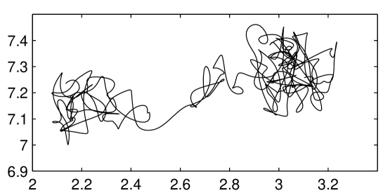
Figure 3.1: Trajectory (in the x-z plane) of a “hopping” particle. First, the particle stays relatively localized for a period of time, seemingly oscillating around a position in the left side of the figure. After this, the particle move more or less directly to a new position in the right of the figure, where it again become localized. The temperature is $T=0.59$, and the elapsed time is $\Delta t=160$ (see later for units of these numbers).

In the work of Wahnström, the system was investigated both above and below the glass-temperature, $T_{g}$, i.e. the system was allowed to fall out off equilibrium as it was cooled. As a consequence, it was unclear whether the hopping seen was a feature of the equilibrium liquid, or if it was a consequence of non-equilibrium dynamics. Here we attempt to keep the system equilibrated at all temperatures, i.e. the equilibration time is made longer and longer as the temperature is lowered.

The “Wahnström system” is a binary mixture of $N=500$ particles, with 50% particles of type A, and 50% particles of type B. The particles interact via the pair-wise Lennard-Jones potential, where the parameters depend on the types of the two particles involved ($\alpha$ and $\beta$):

$$V_{\alpha\beta}(r)=4\epsilon_{\alpha\beta}\left(\left(\frac{\sigma_{\alpha\beta}}{r}\right)^{12}-\left(\frac{\sigma_{\alpha\beta}}{r}\right)^{6}\right)$$ (3.1)

The forces are given by the negative gradient of the potential:

$${\mathbf{F}}_{\alpha\beta}({\mathbf{r}}) = -\nabla V_{\alpha\beta}=-\frac{\partial V_{\alpha\beta}}{\partial r}\frac{{\mathbf{r}}}{r}$$ (3.2)

$$= \frac{48\epsilon_{\alpha\beta}}{(\sigma_{\alpha\beta})^{2}}\left(\left(\frac{\sigma_{\alpha\beta}}{r}\right)^{14}-\frac{1}{2}\left(\frac{\sigma_{\alpha\beta}}{r}\right)^{8}\right){\mathbf{r}}$$ (3.3)

$V_{\alpha\beta}(r)$ is characterized by a minimum at $V_{\alpha\beta}(2^{1/6}\sigma_{\alpha\beta})=-\epsilon_{\alpha\beta}$, steep repulsion at shorter distances, and a weaker attraction at longer distances.

The length-parameters used in the Wahnström system are: $\sigma_{AA}=1$, $\sigma_{BB}=1/1.2\approx 0.833$ and $\sigma_{AB}=(\sigma_{AA}+\sigma_{BB})/2$. The energy-parameters are all identical: $\epsilon_{AA}=\epsilon_{AB}=\epsilon_{BB}=1$. The masses of the particles are given by $m_{A}=2$, and $m_{B}=1$. The length of the sample was $L=7.28$, which gives a (reduced) density of $\rho=N/L^{3}=1.296$. Times are reported in units of $\tau\equiv(m_{B}\sigma_{AA}^{2}/48\epsilon_{AA})^{1/2}$ (This expression contains an error in paper II). When comparing simulations of a model-liquid like the one described here with experimental results for real liquids, it is customary to use “Argon units”, i.e. parameters used when modeling Argon atoms by the Lennard-Jones potential; $\sigma=3.4\AA$, $\epsilon=120Kk_{B}$, and $\tau=3\times 10^{-13}sec$ [17].

The potential is “cut and shifted” [1] at $r=2.5\sigma_{\alpha\beta}$, which means that it is set to zero for $r\geq 2.5\sigma_{\alpha\beta}$, and $|V_{\alpha\beta}(2.5\sigma_{\alpha\beta})|\approx 0.016$ is added to the potential for $r\leq 2.5\sigma_{\alpha\beta}$. This makes the potential continuous at $r=2.5\sigma_{\alpha\beta}$, while the force is not. The equations of motion are integrated with periodic boundary conditions using the Leap-Frog algorithm [1] (which is simply a discretizaition of Newton’s second law) with a time step of $0.01\tau$.

Three independent samples were used, each initiated by generating a random configuration followed by equilibration at a high temperature ($T=5.0$). The cooling was done by controlling the total energy of the system, which was done by scaling the velocities. An equilibration run of length $t_{eq}$ was then performed, followed by a production run of the same length. If the samples was determined not to be equilibrated properly, $t_{eq}$ was doubled, by “degrading” the production run to be part of the equilibration run, and making a new production run twice as long. This procedure was continued until the samples was determined to be equilibrated. The criteria used for determining if the samples were equilibrated will be discussed later. Note, that by this procedure, it is the total energy ($E_{tot}=E_{pot}+E_{kin}$) that is controlled. The reported temperatures and pressures are computed as time-averages over the instantaneous temperature and pressure respectively [1]:

$$T(t) \equiv \frac{2E_{kin}(t)}{3N-3}$$ (3.4)

$$P(t) \equiv \rho T(t)+W(t)/V,~{}~{}~{}W(t)\equiv\frac{1}{3}\sum_{i}\sum_{j>n}{\mathbf{r}}_{ij}\cdot{\mathbf{F}}_{ij}$$ (3.5)

where $W(t)$ is the virial and the summing is over all pair of particles.

Some of the results for the system described above, will be compared with results from a different binary Lennard-Jones mixture (the “Kob & Andersen system”), which has been investigated in a number of papers [34, 17, 18, 35, 36]. This system is a 80:20 mixture, with $\sigma_{AA}=1$, $\sigma_{AB}=0.8$, $\sigma_{BB}=0.88$, $\sigma_{AB}=0.8$, $\epsilon_{AA}=1.0$, $\epsilon_{AB}=1.5$, $\epsilon_{BB}=0.5$, and $m_{A}=m_{B}=1$.

3.2 Static Results

Figure 3.2 shows as a function of temperature a) the potential and total energy per particle, and b) the pressure vs. Temperature. The error-bars are estimated from deviations between the three independent samples, which are found to be in reasonable agreement. This is a necessary (but not sufficient) condition for the system(s) to be equilibrated. Note that its the total energy which was set to be equal for the three samples, and consequently there are small deviations in the measured temperatures.

Figure 3.2: a) Total and potential energy per particle as a function of temperature. b) Pressure vs. temperature. In both a) and b) (as in the following if nothing else is mentioned) error-bars are estimated from deviation between three independent samples.

The specific heat capacity at constant volume, $C_{v}$, is given by [1]:

$$C_{v}=\frac{1}{N}\frac{dE_{tot}}{dT}$$ (3.6)

From figure 3.2a we see that $C_{v}$ increases as the temperature is lowered. Note that there is no indication of a glass-transition, since this would be indicated by a sharp decrease in $C_{v}$ when cooling below the glass transition temperature, $T_{g}$, as seen in the results by Wahnströhm. The heat capacity at constant volume will be discussed further in section 4.2.

In figure 3.3 is shown the pair-correlation functions, $g_{AA}(r)$, $g_{AB}(r)$, and $g_{BB}(r)$, at three of the temperatures simulated. The pair-correlation function, $g_{\alpha\beta}(r)$, is the average relative density of particles of type $\beta$ around particles of type $\alpha$ [37]. It is normalized to be 1 at large distances, $r$, were the correlations disappears. At the highest temperature ($T=1.06$) all three pair-correlation functions is seen to look like ’typical’ high temperature pair-correlation functions, with a sharp first neighbor peak, a more rounded second neighbor peak, etc. As the temperature is lowered the first neighbor peak becomes sharper and the second peak splits into two peaks. The splitting of the second peak upon cooling is often seen in super-cooled liquids (see eg.[15, 17]).

The parameters used in the potential does not energeticly favor the mixture of A and B particles ($\epsilon_{AB}$ is not larger than $\epsilon_{AA}$ and $\epsilon_{BB}$), which might cause the system to phase separate at sufficiently low temperatures. In the event of phase separation, we would expect the area of the first peak in $g_{AB}(r)$ to decrease at the temperature where phase separation starts occurring. There is no indication of this in figure 3.3.

In figure 3.4 is shown the static structure factors, $S_{AA}(q)$, $S_{AB}(q)$, and $S_{BB}(q)$, corresponding to the data shown in figure 3.3. The static structure factor is the (3 dimensional) Fourier transform of pair correlation function, and thus contains the same information. However the finite sample size introduces some features in $S_{\alpha\beta}(q)$ which are clearly unphysical (see eg. [18]). By recalculating $S_{\alpha\beta}(q)$ from $g_{\alpha\beta}(r)$ with a cut-off in $r$ that is less than $L/2$ one can get an idea about which features of $S_{\alpha\beta}(q)$ are due to finite-size effects. Doing this shows, that at $q$-values to the left of the first peak ($q\approx 6$, depending on type of correlation) $S_{\alpha\beta}(q)$ is dominated by finite-size effects, which is why most of it is not shown. Also the small “wiggles” seen at $q\approx 10$ is a finite-size effect. The splitting of the peaks at $q\approx 15$ is however not a finite-size effect.

Figure 3.3: Pair correlation function at a high ($T=1.06$), medium ($T=0.66$), and low temperature ($T=0.59$); a) A-A correlation, $g_{AA}(r)$, b) A-B correlation, $g_{AB}(r)$, c) B-B correlation, $g_{BB}(r)$

Figure 3.4: Static structure factor at a high ($T=1.06$), medium ($T=0.66$), and low temperature ($T=0.59$); a) A-A correlation, $S_{AA}(q)$, b) A-B correlation, $S_{AB}(q)$, c) B-B correlation, $S_{BB}(q)$

3.3 Mean Square Displacement

In figure 3.5 we show the mean square displacement of the a) A particles, $\langle r^{2}(t)\rangle_{A}$, and b) B particles, $\langle r^{2}(t)\rangle_{B}$. At short times ($t<1$) a ballistic regime ($\langle r^{2}(t)\rangle_{\alpha}\propto t^{2}$) is seen for both A and B particles, at all temperatures. The ballistic regime is simply a consequence of the velocities being constant at these short time scales:

$$\langle r^{2}(t)\rangle_{\alpha}~{}=~{}\langle(Vt)^{2}\rangle_{\alpha}~{}=~{}\langle V^{2}\rangle_{\alpha}~{}t^{2}$$ (3.7)

In the insets in figure 3.5 is shown $\langle V^{2}\rangle_{\alpha}$ calculated by eq. 3.7. $\langle V^{2}\rangle_{\alpha}$ can also be calculated directly from the temperature:

$$T=\frac{2E_{kin}}{3(N-1)}=\frac{Nm_{\alpha}\langle(V/\tau)^{2}\rangle_{\alpha}}{3(N-1)}=\frac{48m_{\alpha}\langle V^{2}\rangle_{\alpha}}{3(1-1/N)}$$ (3.8)

In the insets in figure 3.5 is also shown $\langle V^{2}\rangle_{\alpha}$ as calculated from eq. 3.8. The excellent agreement between eq. 3.7 and 3.8 (with no fitting involved) is not a big surprise, but it gives confidence in the argument leading to eq. 3.7, and acts as a consistency check.

In figure 3.5 a diffusive regime ($\langle r^{2}(t)\rangle_{\alpha}\propto t$) is seen at long times, for all temperatures. As the temperature is lowered the time scale at which the diffusive regime sets in increases, and a plateau is seen to evolve between the ballistic and diffusive regimes. This behavior is typical for what is seen in simulations of super-cooled liquids, and the plateau is argued to be associated with particles being trapped in local “cages” consisting of their neighbors [17, 38].

The vertical dashed lines in figure 3.5 identifies the time $t_{1}$, defined by $\langle r^{2}(t_{1})\rangle_{\alpha}=1$. The significance of this time will be discussed in connection with figure 3.6.

Figure 3.5: The mean square displacement of a) the large particles, $\langle r^{2}(t)\rangle_{A}$, and b) the small particles, $\langle r^{2}(t)\rangle_{B}$. Insets show $\langle V^{2}\rangle_{\alpha}$ calculated from eq. 3.7 and 3.8, and demonstrates the agreement between the two equations. The vertical dashed lines identifies $\langle r^{2}(t_{1})\rangle_{\alpha}=1$.

Fitting $\langle r^{2}(t)\rangle_{\alpha}$ in the diffusive regime to the Einstein relation:

$$\langle r^{2}(t)\rangle_{\alpha}~{}=~{}6Dt$$ (3.9)

we determine the diffusion coefficient, $D$, as a function of temperature (and particle type). We postpone the discussion of the temperature dependence of $D$ to section 3.6, where it will be discussed together with other measures of the time scales involved (eg. $t_{1}$). Following Kob and Andersen [17] we in figure 3.6 present the data for $\langle r^{2}(t)\rangle_{\alpha}$ as a function of $6Dt$. In the diffusive regime the data for all temperatures should, according to eq. 3.9, fall on the line $6Dt$, which is seen to be the case for $\langle r^{2}(t)\rangle_{\alpha}\gtrsim 1$. In other words the time $t_{1}$, defined by $\langle r^{2}(t_{1})\rangle_{\alpha}=1$, can be viewed as marking the onset of the diffusive regime. The fact that the diffusive regime is reached at all temperatures (compare fig. 3.5), is a necessary (but not sufficient) condition, for the system(s) to be in equilibrium.

As is the case for the data presented by Kob and Andersen, the data in figure 3.6 seems to indicate a universal behavior; As the temperature is decreased $\langle r^{2}(t)\rangle_{\alpha}$ follows the thick dashed curve in figure 3.6 to lower and lower scaled times. The thick dashed curves are fits to the fitting function used by Kob and Andersen [17] (see table 3.1):

$$\langle r^{2}(t)\rangle_{\alpha}~{}=~{}r_{c}^{2}+A(Dt)^{b}+6Dt$$ (3.10)

The parameter $b$ is the so-called “von-Sweidler” exponent, which is related to the dynamics at intermediate times, i.e. between the plateau and the diffusive regime. According to the asymptotic predictions of the ideal mode coupling theory (MCT) [21, 22], the von-Sweidler exponent, $b$, should be independent of the particle type. Kob and Andersen argue that the two values they find, 0.48 for the A particles and 0.43 for the B particles, are within reasonable agreement. This is not the case for the $b$-values found here; $0.17\pm 0.03$ for the A particles and $0.27\pm 0.01$ for the B particles.

Type	$r_{c}$	$A$	$b$
A	$0.131\pm 0.013$	$0.071\pm 0.002$	$0.17\pm 0.03$
B	$0.166\pm 0.003$	$0.096\pm 0.003$	$0.27\pm 0.01$

Table 3.1: Parameters found by fitting equation 3.10 to the “universal” curves in figure 3.6 (thick dashed lines). Error-bars are 68% confidence intervals, as reported by the fitting routine in Gnuplot.

Figure 3.6: The mean square displacement plotted as function of $6Dt$ (same data as in figure 3.5). For $\langle r^{2}(t)\rangle_{\alpha}\gtrsim 1$ the data for all temperatures fall on the straight dotted line marking diffusive behavior (eq. 3.9). The thick dashed lines are fits to eq. 3.10

3.4 The van Hove Correlation Function

To characterize the dynamics in more detail, we calculate the van Hove self correlation function [37] (where the sum is over particles of type $\alpha$):

$$G_{s\alpha}({\bf r},t)={1\over N_{\alpha}}\sum_{i=1}^{N_{\alpha}}\left<\delta({\bf r}_{i}(t)-{\bf r}_{i}(0)-{\bf r})\right>,$$ (3.11)

which is the probability density of a particle of type $\alpha\in\{A,B\}$ being displaced by the vector ${\bf r}$, during the time interval $t$. In an isotropic system $G_{s\alpha}({\bf r},t)$ does not depend on the direction of $r$, and the probability distribution of a particles being displaced the distance ${r}$ is $4\pi r^{2}G_{s\alpha}({r},t)$. The mean square displacement, $\langle r^{2}(t)\rangle_{\alpha}$, is given by the second moment of $4\pi r^{2}G_{s\alpha}({r},t)$, and the later thus gives a more detailed view of the dynamics.

In figure 3.7 is plotted $4\pi r^{2}G_{sA}(r,t_{1})$ and $4\pi r^{2}G_{sB}(r,t_{1})$, i.e. the distribution of distances moved by A and B particles respectively in the time interval $t_{1}$, which in the previous section was demonstrated to be at the onset of the diffusive regime. The thick curve is the Gaussian approximation:

$$G_{s}(r,t)=\left(\frac{3}{2\pi\langle r^{2}(t)\rangle}\right)^{3/2}\exp\left(-\frac{3r^{2}}{2\langle r^{2}(t)\rangle}\right)$$

which is seen to be reasonably fulfilled at high temperatures. As the temperature is lowered the results starts graduately deviating from the Gaussian approximation, and a shoulder builds at the average inter particle distance, $r\approx 1.0$, which at T=0.59 becomes a well-defined second peak. The second peak, observed also in other model liquids, is interpreted [13, 14, 9, 8, 15, 16, 17] as single particle hopping (see figure 3.1), i.e. the particles stay localized in their local cages a certain time (first peak), then moves more or less directly out to distances approximately equal to the inter particle distance (second peak) (This behavior was also reported in [12]). To what extent the hopping behavior is related to activated hopping over energy barriers will be discussed in chapter 4.

Note that when analyzing the dynamics in more detail by means of the van Hove self correlation function (fig. 3.7), the universality seen in the mean square displacement (fig. 3.6) is completely gone; The way the system “achieves” the diffusive behavior (i.e. the dynamics at $t_{1}$) changes qualitatively from high temperature (Gaussian) to low temperature (Hopping).

Figure 3.7: The distribution of particle displacements, $4\pi r^{2}G_{s\alpha}(r,t_{1})$, where $t_{1}$ is defined by $\langle r^{2}(t_{1})\rangle_{\alpha}=1$, see figure 3.5. At high temperatures the Gaussian approximation (thick curve) is reasonable fulfilled, whereas at the lowest temperature a secondary peak is present, indicating that hopping is present in the system (see text). The small particles (type B) are seen to have a larger tendency to exhibit hopping, compared to the large particles.

Figure 3.8: The non-Gaussian parameters, $\alpha_{2A}(t)$ and $\alpha_{2B}(t)$. The dashed line is a fit to a power-law in the “universal” regime before the maximum.

The deviation from Gaussian behavior is often analyzed in terms of the Non-Gaussian parameter [39, 40, 41, 42, 17, 38, 43, 35]:

$$\alpha_{2}(t)=\frac{\langle r^{4}(t)\rangle-\langle r^{4}(t)\rangle_{Gauss}}{\langle r^{4}(t)\rangle_{Gauss}}=\frac{3\langle r^{4}(t)\rangle}{5\langle r^{2}(t)\rangle^{2}}-1$$ (3.12)

which is the relative deviation between the measured $\langle r^{4}(t)\rangle$ and what it would be for a given value of $\langle r^{2}(t)\rangle$, if $G_{s}(r,t)$ was Gaussian: $\langle r^{4}(t)\rangle_{Gauss}=5\langle r^{2}(t)\rangle^{2}/3$. In figure 3.8 is shown $\alpha_{2}$ for the A and B particles respectively.

Like in [17, 38] we see a universal behavior in the way $\alpha_{2A}(t)$ increases, before it reaches its maximum. Following [38] a power-law fit is done in this regime, from which is found exponents of $0.64$ and $0.67$ for the A and B particles respectively. The exponent found in [38] is $0.4$. As noted in [17] the universality seen in $\alpha_{2}(t)$ is different from the one found in the behavior of $\langle r^{2}(t)\rangle_{\alpha}$ (fig. 3.6); The universality seen in $\alpha_{2}(t)$ does not involve any scaling.

The time $t^{*}$ which is defined as the position of the maximum in $\alpha_{2}(t)$, can be interpreted as the time where the dynamics deviates most from Gaussian behavior [40, 35]. In figure 3.9 is shown for three temperatures, the time development of $4\pi r^{2}G_{sB}(r,t)$. At each temperature $4\pi r^{2}G_{sB}(r,t)$ is shown at a time close to $t^{*}$ (indicated by the arrows), and 2,4,8, and 16 times that time. At $T=1.06$ the distribution of particle displacements is seen to be characterized by a single peak, which “spreads out” without any qualitative change in the shape, as time increases. This is the typical behavior for liquids at high temperatures [37]. At $T=0.66$ the behavior is seen to be qualitatively similar, except for a weak indication of a shoulder at $r\approx 1.0$. The time development of $4\pi r^{2}G_{sB}(r,t)$ at $T=0.59$ is qualitatively different from what is found at higher temperatures; The first peak decreases while the position is almost constant, and at the same time as the second peak starts building up. This supports the “hopping” interpretation of the second peak given above; The particles escape their local “cages” (the first peak), by “suddenly appearing” at approximately the inter particle distance (second peak). After the last time shown here, the second peak starts decreasing. This is interpreted as a consequence of particles hopping again.

With the regards to the interpretation of $t^{*}$ mentioned above, one should note that for $T=0.59$ the second peak in $4\pi r^{2}G_{sB}(r,t)$ builds up after the time $t^{*}$, i.e. after $\alpha_{2}(t)$ has its maximum. A more detailed analysis of the non-Gaussian behavior should include the higher order analogues of $\alpha_{2}(t)$ (involving higher moments of $4\pi r^{2}G_{s\alpha}(r,t)$) [39], but this approach will not be pursued further here.

Figure 3.9: Time development of the distribution of particle displacements for the B particles, $4\pi r^{2}G_{sB}(r,t)$, at the same temperatures as in figure 3.3. At each temperature $4\pi r^{2}G_{sB}(r,t)$ is shown at a time close to $t^{*}$ (smallest time indicated by arrows), and 2,4,8, and 16 times that time.

The van Hove distinctive correlation function, $G_{D\alpha\beta}(r,t)$, is the time dependent generalization of the pair correlation function [13]:

$$G_{D\alpha\beta}({\bf r},t)={1\over\sqrt{N_{\alpha}N_{\beta}}}\sum_{i=1}^{N_{\alpha}}\sum_{j=1}^{N_{\beta}}\left<\delta({\bf r}_{j}(t)-{\bf r}_{i}(0)-{\bf r})\right>,$$ (3.13)

where the first sum is over particles of type $\alpha$, the second sum is over particles of type $\beta$, and $i\neq j$ if $\alpha=\beta$ (this last term is contained in $G_{s\alpha}(r,t)$, see equation 3.11). $G_{D\alpha\beta}(r,t)$ is the relative density at time $t$ of $\beta$-particles at ${\bf r}$, given that there at time $t=0$ was a $\alpha$-particle at ${\bf r}=0$ (normalised to be 1 if there is no correlation).

In figure 3.10 is shown $G_{DBB}(r,t)$ for the same temperatures and times as in figure 3.9. Included in figure 3.10 is also $G_{DBB}(r,t=0)=g_{BB}(r)$. Except for the lowest values of $r$, the features of the pair correlation function is seen to approach the long-time value $G_{D\alpha\beta}(r,t)=1$ in a smooth manner, which is the typical high-temperature behavior [37]. As the temperature is decreased, a significant “overshoot” develops at the small $r$-values, indicating that there is an excess probability that when a particle jumps, it does so to a position previously occupied by another particle. Thus, while $G_{sB}(r,t)$ (fig. 3.9a) shows that particles has a tendency to jump a distance approximately equal to the inter-particle distance, $G_{D\alpha\beta}(r,t)$ give the further information, that they have a tendency to jump to a position previously occupied by another particle. Similar (but less pronounced behavior) was found in [13].

In a scenario where the dynamics is dominated by particles jumping to positions previously occupied by other particles, one should expect that moving particles make up correlated string-like objects in the liquid. This kind of behavior is found by Muranaki and Hiwatari in a soft sphere system [44], and by Donati et. al. in the Kob & Andersen system [36]. This type of behavior will be discussed further in chapter 4.

Figure 3.10: Time development of $G_{DBB}(r,t)$ for the same temperatures as in figure 3.9. For each temperature, the times used here are the same as in figure 3.9, and $t=0$ (thick dotted curve), where $G_{DBB}(r,t=0)$ equals the pair correlation function, $g_{BB}(r)$.

3.5 The Intermediate Scattering Function

The self part of the intermediate scattering function, $F_{s}(q,t)$, is the (3 dimensional) Fourier transform of the van Hove self correlation function [37]:

$$F_{s}({\mathbf{q}},t) \equiv \int G_{s}({\mathbf{r}},t)e^{-i\mathbf{q}\cdot\mathbf{r}}d\mathbf{r}~{}=~{}\langle\cos{{\mathbf{q}}({\mathbf{r}}_{j}(t)-{\mathbf{r}}_{j}(0))}\rangle$$ (3.14)

$F_{s}(q,t)$ is a relaxation function, normalized to be 1 at $t=0$, and it goes to zero for $t\rightarrow\infty$. Figure 3.11 shows the self part of the intermediate scattering function for the A particles and B particles; $F_{sA}(q_{maxA}=7.5,t)$ and $F_{sB}(q_{maxB}=8.1,t)$. $q_{maxA}=7.5$ and $q_{maxA}=8.1$ are here the positions of the first peak in the static structure factor for the A-A correlation ($S_{AA}(q)$), and the the B-B correlation ($S_{BB}(q)$), respectively (see figure 3.4). As the temperature is lowered a two-step relaxation develops, which is what is typically seen in glass-forming liquids, both in experiments [46] and in simulations [14, 15, 45, 47, 34, 18, 42, 48, 38, 49, 43]. The initial relaxation is a consequence of the particles oscillating in their cages, while the the long-time (alpha) relaxation is a consequence of particles escaping their cages [45, 42, 38]. The alpha relaxation is often found to be well approximated by stretched exponentials, $f(t)=f_{c}\exp(-(t/\tau_{\alpha})^{\beta})$ [14, 15, 34, 18, 42, 38], which is also the case in figure 3.11, where fits to stretched exponentials are shown as dashed lines.

In Fig. 3.12 we show as a function of temperature the three fitting parameters used in figure 3.11; a) relaxation times, $\tau_{\alpha}$, b) stretching parameters, $\beta$, and c) non-ergodicity parameters $f_{c}$. As expected the relaxation times, $\tau_{\alpha A}$ and $\tau_{\alpha B}$ is seen to increase dramatically as the temperature is lowered. The asymptotic prediction of the ideal mode-coupling theory (MCT) is $\tau_{\alpha}=\tau_{0}(T-T_{c})^{-\gamma}$ [21, 22]. The divergence of $\tau_{\alpha}$ at $T_{c}$ predicted by the ideal MCT is never seen in practice. This is argued to be consequence of relaxation by hopping taking over close to $T_{c}$ [21, 15, 17, 50, 22]. This means that close to $T_{c}$ the power-law is expected to break down and it should not be fitted in this regime. Unfortunately we have no independent estimate of $T_{c}$, and furthermore it is not known how close to $T_{c}$ the power-law is expected to hold. Since we have already demonstrated, that hopping is present in the system at the lowest temperatures, we can expect that these are close to $T_{c}$, which means that we might run into the problem described above. We note also, that the power-law is an asymptotic prediction, i.e. it is expected to break down at high temperatures, but again it is not known how far from $T_{c}$ this is supposed to happen.

Figure 3.11: a) The self part of the intermediate scattering function for the A particles, $F_{sA}(q_{maxA}=7.5,t)$. The dashed lines are fits to stretched exponentials, $f(t)=f_{c}\exp(-(t/\tau_{\alpha})^{\beta})$. The fitting was performed for $t>10$ for the 2 highest temperatures, and for $t>30$ for the rest of the temperatures. b) $F_{sB}(q_{maxB}=8.1,t)$, otherwise as above.

Figure 3.12: Fitting parameters used in figure 3.11. a) Relaxation times $\tau_{\alpha A}$ and $\tau_{\alpha B}$. The lines are fits to $\tau_{\alpha}\propto(T-T_{c})^{-\gamma}$ (see text). b) Stretching parameters $\beta_{A}$ and $\beta_{B}$. c) Non-ergodicity parameters, $f_{cA}$ and $f_{cB}$.

As discussed above, the temperature range (if any) where the asymptotic predictions of ideal MCT is supposed to hold, is not known. Consequently the following approach for fitting $\tau_{\alpha}=\tau_{0}(T-T_{c})^{-\gamma}$ has been applied; First the fit was done for all 8 temperatures ($T_{cut}=0$), then by excluding the lowest temperature ($T_{cut}=0.60$), and then by excluding the two lowest temperatures ($T_{cut}=0.63$).

The results of the fitting-procedure described above, is seen in table 3.2. For both the A and B particles the parameters found for $T_{cut}=0.60$ and $T_{cut}=0.63$ agree within the error-bars, while they disagree with the parameters for $T_{cut}=0$. Thus one might argue that the parameters found for $T_{cut}=0.60$ and $T_{cut}=0.63$ describes the “true” power-law, while the fit found using $T_{cut}=0$ deviates as a consequence of fitting too close to $T_{c}$. Thus our best attempt at a power-law fit is the one achieved for $T_{cut}=0.60$ (i.e. by excluding the lowest temperature), which is the fit shown in figure 3.12 for the A and B particles respectively. The values estimated in this manner for $T_{c}$ and $\gamma$ for the A and B particles are identical within the error-bars, as predicted by the ideal MCT. The temperature dependence of $\tau_{\alpha}$ will be discussed further in section 3.6.

Type	$T_{cut}$	$\tau_{0}$	$T_{c}$	$\gamma$
A	$0.00$	$4.2\pm 0.6$	$0.571\pm 0.004$	$1.71\pm 0.10$
A	$0.60$	$5.4\pm 0.5$	$0.592\pm 0.004$	$1.41\pm 0.07$
A	$0.63$	$5.3\pm 0.4$	$0.586\pm 0.008$	$1.46\pm 0.09$
B	$0.50$	$2.9\pm 0.5$	$0.571\pm 0.004$	$1.77\pm 0.11$
B	$0.60$	$3.7\pm 0.4$	$0.592\pm 0.005$	$1.47\pm 0.09$
B	$0.63$	$3.6\pm 0.4$	$0.584\pm 0.010$	$1.52\pm 0.12$

Table 3.2: Parameters found by fitting $\tau_{\alpha}=\tau_{0}(T-T_{c})^{-\gamma}$ to all 8 temperatures ($T_{cut}=0$), excluding the lowest temperature ($T_{cut}=0.60$), and by excluding the two lowest temperatures ($T_{cut}=0.63$). The error-bars indicate the 68.3% confidence interval, as reported by Gnuplot.

The numerical data for $\tau_{\alpha}(T)$ does not by itself give strong evidence for a dynamical transition at the estimated $T_{c}=0.592\pm 0.004$; nothing special seems to happen at that temperature. However, the agreement with the lowest temperature ($T=0.591\pm 0.002$), where we clearly see hopping (figure 3.7), gives us confidence that there is a dynamical transition close to the estimated $T_{c}$.

The stretching parameters, $\beta_{A}$ and $\beta_{B}$, are seen in figure 3.12b to decrease from values close to 1 (i.e. exponential relaxation) at high temperatures, to values close 0.5 at the lowest temperatures. The values found at high-temperatures are somewhat dependent on the time-interval used for the fitting, and the real error-bars are thus bigger than the ones shown (which are estimated from deviations between the three independent samples, with the fitting done in the same time-intervals). However focusing on the medium to low temperatures ($T\lesssim 0.73$), there can be no doubt that $\beta$ is increasing as function of temperature. This is in contradiction with the asymptotic predictions of the ideal MCT, which predicts $\beta$ to be constant. The ideal MCT does not directly predict the long-time relaxation to be stretched exponentials, but it predicts it to exhibit time-temperature super-position (TTSP) [21, 22]. This mean that the shape of the long-time relaxation should be independent of temperature, which for stretched exponentials means that $\beta$ should be constant.

Figure 3.13: (a) The self part of the intermediate scattering function for the A particles, $F_{sA}(q=7.5,t)$, scaled to test if the long-time relaxation exhibits time-temperature super-position. This is not the case.

The question of whether $\beta$ is constant or increases towards 1 has led to controversy about what is the right fitting procedure [50, 51]. Another way of checking for TTSP, is by scaling the data appropriately and look for approach to an universal curve. This is done in figure 3.13 where $F_{sA}(q_{max},t)/f_{cA}$ is plotted versus $t/\tau_{\alpha A}$ which should be identical for any temperature range where TTSP holds. No such temperature range can be identified. One might argue, that the scaling approach used in figure 3.13 relies on the values of $f_{c}$ estimated from the fits to stretched exponentials, which at the high temperatures is dependent on the time-range chosen for the fitting. Scaling $F_{sA}(q_{max},t)$ to agree at $F_{sA}(q_{max},t)=e^{-1}$ (i.e. without dividing by $f_{c}$), like done in [18] does not change the conclusion above; there is no indication of TTSP.

The fact that $F_{s\alpha}(q,t)$ decays to zero (figure 3.11), and that the parameters describing the alpha relaxation is in reasonably agreement for the three independent samples (as illustrated by the error-bars in figure 3.12), are necessary conditions for the liquid to be in equilibrium. Of all tests for equilibrium applied, this was the one that was found to be most sensitive, i.e. requiring the longest equilibration times.

In figure 3.14 is plotted $F_{sA}(q,t)$ at $T=0.59$ for $q$-values $1,2,...,20$, and $q=q_{max}=7.5$ (thick dashed line). Also shown in figure 3.14 are fits to stretched exponentials (dashed lines). The fitting parameters used in 3.14 is plotted in figure 3.15. At the lowest $q$-values the fits are not perfect, but except for that the fits are reasonable. Note that in the time-range were the second peak builds up in $4\pi r^{2}G_{sA}(r,t)$, i.e. from $t^{*}\approx 6\cdot 10^{2}$ to $t_{1}\approx 7\cdot 10^{3}$, figure 3.14 shows no clear indication of this. Since $F_{s\alpha}(q,t)$ is the Fourier transform of $G_{s\alpha}(r,t)$, and thus contains the same information, it is possible to extract the information about the hopping from $F_{s\alpha}(q,t)$. However since we already have an excellent indication of the hopping in $4\pi r^{2}G_{s\alpha}(r,t)$, and $G_{D\alpha\beta}(r,t)$, this will not be pursued further here.

Figure 3.14: The self part of the intermediate scattering function for the A particles, $F_{sA}(q,t)$, at $T=0.59$ for $q$-values $1,2,...,20$, and $q=q_{max}=7.5$ (thick dashed line). Thin dashed lines are fits to stretched exponential, where the fitting was done for $t\geq 30$.

Figure 3.15: q-dependence of parameters found by fitting stretched exponentials to $F_{sA}(q,t)$, at $T=0.59$, see figure 3.14

3.6 Time Scales

In this section, we compare the measures of time-scales found in the previous sections. In figure 3.16 is plotted $(6D)^{-1}$ (squares, from figure 3.5), $t_{1}$ (plus, from figure 3.5), $t_{\alpha}$ (diamonds, from figure 3.12), and $t^{*}$ (circles, from figure 3.8). If $t_{1}$ is in the diffusive regime, the relation $(6D)^{-1}=t_{1}$ should hold, see equation 3.9. This is seen in figure 3.16 to hold to a good approximation; the largest deviation is 8%, with $t_{1}$ being smaller than $(6D)^{-1}$, thus confirming that $t_{1}$ is a good estimate of the onset of the diffusive regime, as argued in section 3.3. $t^{*}$ is found to be roughly a factor $10$ smaller than $t_{1}$, and $(6D)^{-1}$ (the ratio changes from roughly 6 at high temperatures, to roughly 11 at low temperatures). Also shown in figure 3.16 are attempts to fit $(6D)^{-1}$ to a power-law. According to the asymptotic predictions of ideal MCT, $(6D)^{-1}$ should have the same temperature dependence as $\tau_{\alpha}$ (apart from a constant factor), which means that we should find the same $T_{c}$ and $\gamma$. Consequently the fitting was done in the temperature range which gave the “best” power-law fit to $\tau_{\alpha}$, i.e. by excluding the lowest temperature. This fit is shown, for the A and B particles respectively, as the full curves in figure 3.16, and the parameters and error-bars are given in table 3.3. The fit to the data are reasonable, but the estimated $T_{c}$ deviates from the one found from $\tau_{\alpha}$, which is in contradiction with MCT. The dashed curves in figure 3.16 are the results of power-law fits where $T_{c}$ was set to have the value found for $\tau_{\alpha}$, $T_{c}=0.592$. This also fits the data reasonable, but now the exponents $\gamma$ are different from the ones found from $\tau_{\alpha}$, thus illustrating that $\tau_{\alpha}$ and $(6D)^{-1}$ has different temperature dependence (as can be seen directly in figure 3.16). Also Kob and Andersen find different temperature dependence for the diffusion and the relaxation [34, 17].

Type	$T_{cut}$	$\tau_{0}$	$T_{c}$	$\gamma$
A	$0.60$	$43\pm 3$	$0.574\pm 0.005$	$1.40\pm 0.09$
A	$0.60$	$53\pm 4$	$0.592$	$1.18\pm 0.03$
B	$0.60$	$34\pm 2$	$0.573\pm 0.003$	$1.33\pm 0.05$
B	$0.60$	$42\pm 3$	$0.592$	$1.11\pm 0.03$

Table 3.3: Parameters found by fitting $(6D)^{-1}=\tau_{0}(T-T_{c})^{-\gamma}$, excluding the lowest temperature ($T_{cut}=0.60$). The second set of parameters for each type of particles is for $T_{c}$ being forced to have the value found for $\tau_{\alpha}$, $T_{c}=0.592$. The error-bars indicate the 68.3% confidence interval, as reported by Gnuplot.

Figure 3.16: Time-scales vs. temperature; $(6D)^{-1}$ (squares, from figure 3.5), $t_{1}$ (plus, from figure 3.5), $t_{\alpha}$ (diamonds, from figure 3.12), and $t^{*}$ (circles, from figure 3.8). The lines are power-law fits to $(6D)^{-1}$ (see text).

Figure 3.17: Arrhenius plot of the relaxation times, $\tau_{\alpha}$. Full curves: fits to the Vogel-Fulcher law (see table 3.4), extrapolated to the laboratorie glass-transition (see text). Dashed curves: power-law fits from figure 3.12.

Figure 3.17 shows the alpha relaxation times $\tau_{\alpha A}$ and $\tau_{\alpha B}$, in the so-called “Arrhenius-plot”, i.e. as a function of $1/T$ and with a logarithmic y-axis. In this plot, a Arrhenius dependence of the relaxation time, $\tau_{\alpha}=\tau_{0}\exp(E/T)$ would give a straight line, which is clearly not the case. Or in the terminology of Angel [52], the liquid is “fragile” (non-Arrhenius), as opposed to “strong” (Arrhenius). Included as full lines in figure 3.17 are fits to the Vogel-Fulcher law, $\tau_{\alpha}=\tau_{0}\exp(A/(T-T_{0}))$, which is often seen to fit the relaxation times over a range of temperatures in experiments. The fits are extrapolated, to include the time $\tau_{\alpha}\approx 3\cdot 10^{15}$ which in Argon units (see section 3.1) corresponds to $\tau_{\alpha}\approx 10^{3}$ seconds, i.e. including the time scales involved in the laboratory glass-transition (see introduction). This extrapolation over 12 decades in time (from information covering 2.5 decades), should of course not be taken too seriously, but is included here to illustrate the large differences in time scales. Included as dashed lines in figure 3.17 are the power-law fits from figure 3.12.

Type	$\tau_{0}$	$A$	$T_{0}$
A	$5.2\pm 0.9$	$0.68\pm 0.07$	$0.486\pm 0.009$
B	$3.5\pm 0.7$	$0.70\pm 0.08$	$0.486\pm 0.010$

Table 3.4: Parameters found by fitting the relaxation times, $\tau_{\alpha A}$ and $\tau_{\alpha B}$ to the Vogel-Fulcher law, $\tau_{\alpha}=\tau_{0}\exp(A/(T-T_{0}))$.

3.7 Finite Size Effects

To estimate finite size-effects we in this section present results from a sample with $N=1000$ particles which is otherwise equivalent with the samples described in the previous sections (i.e. same density and total energy per particle).

Figure 3.18 shows the self part of the intermediate scattering function for the A particles for the N=1000 system, together with fits to stretched exponential (dashed lines), using the same fitting procedure as for the N=500 samples (figure 3.11). The resulting fitting parameters are shown in figure 3.19 together with those found for N=500 (figure 3.12). The results for the two system sizes are seen to be in reasonable agreement, indicating that the results in the previous sections do not depend strongly on system size. In [53] a decrease in $\tau_{\alpha}$ by a factor of $\approx 30$ was found at low temperatures for a soft sphere system by going from $N=108$ to $N=10000$. At the moment it is unclear if this much larger change in relaxation time is due to the larger difference in system size, starting from a smaller system, or other differences between the two systems.

Figure 3.18: a) The self part of the intermediate scattering function for the A particles, $F_{sA}(q_{maxA}=7.5,t)$ for a sample with N=1000 particles (compare figure 3.11, $T=0.62$ (second lowest) and $T=0.66$ (fourth lowest) are missing).

Figure 3.19: Fitting parameters used in figure 3.18 for the N=1000 sample. a) Relaxation times $\tau_{\alpha A}$. Power-law reproduced from fig. 3.11a. b) Stretching parameters $\beta_{A}$. c) Non-ergodicity parameters, $f_{cA}$.

3.8 Conclusions

The original motivation for investigating the binary Lennard-Jones system described here, was that it was already demonstrated to exhibit hopping [15]. The first goal of the present work was to test if the hopping was still there if the cooling was done under (pseudo-) equilibrium conditions. Unfortunately there is not a single condition that is known to be sufficient for the system to be equilibrated. The different possibilities include: No drift in static properties (temperature, potential energy, pressure, etc.), long time dynamics being diffusive, relaxation functions such as $F_{s}(q,t)$ decaying to zero. These are all necessary conditions, but none of them are (known to be) sufficient. In the present work, it was found that the most sensitive condition (i.e. requiring the longest equilibration time), was that $F_{s}(q,t)$ decays to zero, and that it does so in the same manner for the three independent samples, i.e. with the relaxation time and stretching exponent being within reasonable agreement. Assuming that this condition is sufficient, it is concluded that the liquid is in equilibrium at all the temperatures presented here, and thus that the hopping found is a feature of the equilibrium liquid.

Although it was not a goal in itself to test the ideal mode coupling theory (MCT), the results of the simulations was compared to the asymptotic predictions of ideal MCT. This was done for two reasons; I) It provides a convenient way of comparing results with other simulations (e.g. Kob and Andersen [34, 17, 18]). II) It is “common” belief that ideal MCT breaks down when hopping dynamics takes over, and the critical mode coupling temperature $T_{c}$ thus constitutes an estimate of when hopping should start to dominate the dynamics. At first hand the last point seems to work fine; the best attempt at a power-law fit to $\tau_{\alpha}$ gives $T_{c}=0.592\pm 0.004$, which is close to the lowest of the temperatures simulated, where we clearly see hopping (figure 3.7). The fact that hopping also is present at the second lowest temperature, might then be taken as an indication that dynamical transition from the “MCT regime” to the “hopping regime” is not a sharp transition, but takes place over some temperature interval. However, the big problem with this scenario is the failure to identify any temperature range, where the asymptotic predictions of ideal MCT holds; There is no indication of TTSP, and the temperature dependence of the time-scales for diffusion and relaxation are clearly different.

In the full version of ideal MCT (as opposed to the asymptotic predictions used in the present work), the exponents of the power-laws discussed here4 are not free parameters, but are determined from the static structure factor [21, 54, 22]. Calculating the exponents from the static structure factor is however a difficult numerical task, which has only been done for a few systems [54]. This has not been attempted for the system used here. In an attempt to include the hopping dynamics in MCT, the so-called extended mode coupling theory has been developed introducing an “hopping-parameter”, as a extra fitting parameter [22]. It has not been attempted to apply extended MCT to the system investigated here.

Chapter 4 Inherent Dynamics

The dynamics of the model glass-forming liquid described in the previous chapter, is here analyzed in terms of its “inherent structures”, i.e. local minima in the potential energy. In particular, we compare the self part of the intermediate scattering function, $F_{s}(q,t)$, with its inherent counterpart $F_{s}^{I}(q,t)$ calculated on a time series of inherent structures. $F_{s}^{I}(q,t)$ is defined as $F_{s}(q,t)$ except that the particle coordinates at time $t$, are substituted with the particle coordinates in the corresponding inherent structure, found by quenching the equilibrium configuration at time $t$. We find that the long time relaxation of $F_{s}^{I}(q,t)$ can be fitted to stretched exponentials, as is the case for $F_{s}(q,t)$. Comparing the fitting parameters from $F_{s}(q,t)$ and $F_{s}^{I}(q,t)$ we conclude, that below a transition temperature, $T_{x}$, the dynamics of the system can be separated into thermal vibrations around inherent structures and transitions between these.

The main conclusions of this chapter can be found in paper III. In the present chapter we introduce the concepts of “energy landscape” and “inherent dynamics”, followed by a summary of paper III. Following this the data shown in paper II  and some additional data is discussed, and a conclusion is given.

4.1 The Potential Energy Landscape

The potential energy landscape [19, 55, 56, 57, 58, 20, 59, 60, 61, 62, 63, 64] of an atomic system (i.e. particles without internal degrees of freedom) is simply the potential energy, as a function of the $3N$ particle coordinates. Letting $\mathbf{R}$ denote the $3N$ dimensional vector describing the state point of the system (i.e. its position in the $3N$ dimensional configuration space), we write the energy landscape as $U(\mathbf{R})$, see figure 4.1. The behavior of the system can be viewed in terms of the state point, $\mathbf{R}(t)$, moving on the energy landscape surface, $U(\mathbf{R})$. This surface contains a large number of minima, termed “inherent structures” by Stillinger and Weber [56]. The inherent structures are characterized by zero gradients in the potential, and they are thus mechanically stable configurations. The inherent structures are separated by saddle points acting as energy barriers. Each inherent structure has a basin of attraction, in which a local minimization of the potential energy (a “quench”) will map the state point $\mathbf{R}(t)$ to the corresponding inherent structure $\mathbf{R}^{I}(t)$.

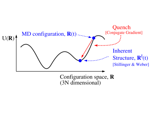
Figure 4.1: Basic concepts in the potential energy landscape. The energy landscape, $U(\mathbf{R})$, contains a large number ($\propto\exp{(kN)}$ [55]) of inherent structures, which are local minima in $U(\mathbf{R})$. Any configuration $\mathbf{R}(t)$ can be mapped by a quench (local minimization of the potential energy), into a corresponding inherent structure, $\mathbf{R}^{I}(t)$. The fact that the $3N$-dimensional configuration space is drawn here as 1-dimensional can be misleading; the configuration space is $3N$-dimensional, and should be thought of as such (difficult as it might be). One might think of the x-axis in this plot as a particular direction in configuration space, connecting two inherent structures. It should not be thought of as an order-parameter (Readers who find this last sentence strange can safely ignore it).

So far all we have done is defining the energy landscape. For a system like the binary Lennard-Jones mixture investigated in the previous chapter we know $U(\mathbf{R})$ exactly; its simply the sum of the pair-potentials (equation 3.1). Of course having a well-defined quantity only helps, if it can tell us something about what we are interested in, i.e. in this case the dynamics of a glass-forming liquid. This is the main question we deal with in this chapter. First we note that for the simulations presented in the previous chapter, the dynamics is governed by Newton’s second law, which using the concepts introduced above can be written as:

$$\frac{d^{2}}{dt^{2}}\mathbf{R}(t)=-\mathbf{M}^{-1}\nabla U(\mathbf{R}(t))$$ (4.1)

where $\mathbf{M}$ is a ($3N$x$3N$) diagonal matrix, with the appropriate masses on the diagonal. In this sense the dynamics is defined by the energy landscape. This is however obviously not telling us anything new. What we want to know is, can we think of the dynamics in terms of the following scenario; the dynamics of the liquid is separated into (thermal) vibrations around inherent structures and (thermally activated) transitions between these. Presented with this scenario, one might very well ask: How can a system with constant total energy (e.g. the system simulated in the previous chapter) perform thermally activated processes? The answer is that one should think of the transitions between inherent structures as involving only a few (local) degrees of freedom, while the remaining degrees of freedom provides the heath bath.

In his classic paper from 1969 Goldstein [19] argued that there exists a transition temperature, which we will term $T_{x}$, below which the flow of viscous liquids is dominated by potential barriers high compared to thermal energies, while above $T_{x}$ this is no longer true. Or in other words; below $T_{x}$ the dynamics is governed by the “vibrations plus transitions” scenario given above. Goldstein gave as a (very) rough estimate, that the shear relaxation time at $T=T_{x}$ is on the order of $10^{-9}$ seconds. Later it was noted by Angell [65], that experimentally it is often found that the shear relaxation time is on the order of $10^{-9}$ seconds at the mode coupling temperature, $T_{c}$. This lead to the argument that Goldstein’s transition temperature, $T_{x}$, is identical to the mode coupling temperature, $T_{c}$. A similar argument was recently given by Sokolov [66].

Figure 4.2: a) Mean value of the quenched energy, $\langle E_{quench}\rangle$ per particle, as a function of temperature. b) The heat capacity at constant volume, $C_{v}(T)$, and the corresponding “quenched heat capacity”, $C_{quench}(T)$ (see text).

Recently, Sastry, DeBenedetti and Stillinger [61] demonstrated that the onset of non-exponential relaxation ($\beta<1$) in a simulated glass-forming Lennard-Jones liquid is associated with a change in the system’s exploration of its potential energy landscape. In figure 4.2a we present data similar to the data presented in [61]. $\langle E_{quench}\rangle(T)$ is here the mean value of the energy of inherent structures, found by quenching configurations from a normal MD run equilibrated at the temperature $T$. Like in [61] we find that this approaches a constant value at high temperatures, where the relaxation becomes exponential ($\beta\approx$ 1, compare fig. 3.12). Similar results was found in [67] for the quenched enthalpy (letting the volume change during the quench).

When plotting the total energy per particle, $E_{tot}(T)/N$ (in figure 3.2), we found that the specific heat capacity at constant volume, $C_{v}(T)$, increases as the system is cooled. In figure 4.2b this is shown explicitly, with $C_{v}(T)$ calculated from eq. 3.6 (using central differences). Also shown in figure 4.2b is the “quenched heat capacity”, $C_{quench}(T)$, calculated in the same way, but with $\langle E_{quench}\rangle(T)$ substituted for $\langle E_{tot}\rangle(T)$. Clearly the increase in $C_{v}(T)$ upon cooling is related to the increase in $C_{quench}(T)$.

4.2 The Inherent Dynamics

The basic idea of the “inherent dynamics” approach is the following (see figure 4.3); After equilibration at a given temperature, a time series of configurations, ${\mathbf{R}}(t)$, is produced by a normal MD simulation. Each of the configurations in ${\mathbf{R}}(t)$ is now quenched, to produce the corresponding time series of inherent structures, ${\mathbf{R}}^{I}(t)$. We now have two “parallel” time series of configurations. The time series ${\mathbf{R}}(t)$ defines the “true dynamics”, which is simply the normal (Newtonian) MD dynamics as presented in the previous chapter, described by $\langle r^{2}(t)\rangle$, $F_{s}(q,t)$, etc. In a completely analogous way, we define the “inherent dynamics” as the dynamics described by the time series ${\mathbf{R}}^{I}(t)$. In other words: If a function describing the true dynamics (eg. $\langle r^{2}(t)\rangle$ or $F_{s}(q,t)$) is calculated by $f({\mathbf{R}}(t))$, then the corresponding function in the inherent dynamics (eg. $\langle r^{2}(t)\rangle^{I}$ or $F_{s}^{I}(q,t)$) is calculated in exactly the same way, except using the time series of inherent structures: $f({\mathbf{R}^{I}}(t))$.

If the true dynamics can be separated into vibrations around inherent structures, and transitions between these, as stated in the “vibrations plus transitions” scenario given above, then the inherent dynamics can be thought of as what is left after the thermal vibrations is removed from the true dynamics.

In the bottom part of figure 4.3 the inherent dynamics approach is applied to the trajectory of the hopping particle, which was shown in figure 3.1; All the configurations that were used to plot the true trajectory were quenched, and the position of the particle in the resulting time series of inherent structures is plotted as the “inherent trajectory”. The quenching procedure is seen to remove the vibrations in the true trajectory. The motion that seems to be left from the vibrations (eg. a jump from $x\approx 2.2$ to $x\approx 2.4$) will be discussed in section 4.5.

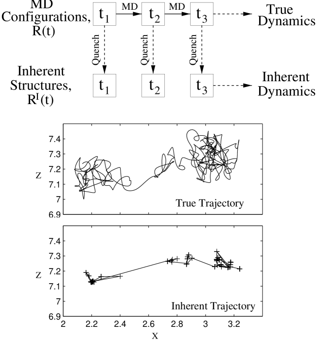
Figure 4.3: Schematic describing the principle of the “inherent dynamics” approach. A time series of configurations ${\bf R}(t)$ of the equilibrated liquid is generated using normal (Newtonian) MD. Configurations in ${\bf R}(t)$ are quenched to produce their corresponding inherent structures ${\bf R}^{I}(t)$. Successive inherent structures then form a time series which we use to calculate “inherent dynamical” quantities such as the inherent mean square displacement, $\langle r^{2}(t)\rangle^{I}$, and the inherent intermediate scattering function, $F_{s}^{I}(q,t)$. Bottom part of the figure: Applying the inherent dynamics approach to the trajectory of a hopping particle (see text).

Paper II and III explores the possibilities of comparing the true and inherent dynamics of the model glass-former described in the previous chapter. The concept of inherent dynamics was first introduced in paper II (without using that name). In that paper the true and inherent versions of the mean square displacement and the van Hove correlation function, was compared on a qualitatively level. Paper III compares the true and inherent version of the self part of the intermediate scattering function, which can be done on a quantitative level by means of stretched exponentials (see section 3.5). This turns out to have important consequences, which is why we here discuss this paper first.

4.3 Paper III

In this paper the concept of inherent dynamics is applied to the self part of the intermediate scattering function, i.e. we compare $F_{s}({q_{max}},t)$, with its inherent counterpart $F_{s}^{I}({q_{max}},t)$. As explained above $F_{s}^{I}({q},t)$ is defined in the same way as $F_{s}({q},t)$, except that the normal particle coordinates, ${\mathbf{r}}_{j}(t)$, are substituted by the corresponding coordinates in the inherent structures, ${\mathbf{r}}^{I}_{j}(t)$ (compare equation 3.14):

$$F_{s}^{I}({\mathbf{q}},t) \equiv \langle\cos{{\mathbf{q}}({\mathbf{r}}^{I}_{j}(t)-{\mathbf{r}}^{I}_{j}(0))}\rangle$$ (4.2)

In figure 4b in paper III $F_{s}^{I}({q_{max}},t)$ is plotted for the A particles, at the 8 temperatures studied. Here we plot the similar data for the B particles in figure 4.4. In both cases we find that the long time relaxation of $F_{s}^{I}({q_{max}},t)$ can be fitted to stretched exponentials, like is the case for $F_{s}({q_{max}},t)$. This is an important finding, since it enables us to make an quantitative comparison between $F_{s}({q_{max}},t)$ and $F_{s}^{I}({q_{max}},t)$, by comparing the two sets of fitting parameters. In the following, the set of fitting parameters for $F_{s}({q_{max}},t)$ is denoted $\{\tau_{\alpha},\beta,f_{c}\}$, while the corresponding set for $F_{s}^{I}({q_{max}},t)$ is denoted $\{\tau_{\alpha}^{I},\beta^{I},f_{c}^{I}\}$

Figure 4.4: The self part of the inherent intermediate scattering function for the B particles, $F_{sB}^{I}(q=8.1,t)$, corresponding to figure 3b in paper III. The dotted lines are fits to stretched exponentials: $f^{I}(t)=f_{c}^{I}\exp(-(t/\tau^{I}_{\alpha})^{\beta^{I}})$

The key question now is: If the true dynamics follows the “vibrations plus transitions” scenario, i.e. if the dynamics can be separated into vibrations around inherent structures, and transitions between these, how is $\{\tau_{\alpha}^{I},\beta^{I},f_{c}^{I}\}$ expected to be related to $\{\tau_{\alpha},\beta,f_{c}\}$? To answer this question, we assume that the initial relaxation in $F_{s}({q},t)$ is due to vibrations, which is the widely accepted explanation (see section 3.5). If this is the case, then we expect the quenching procedure to remove the initial relaxation (since it removes the vibrations), which means that $F_{s}^{I}({q},t)$ can be thought of as $F_{s}({q},t)$ with the initial relaxation removed. This in turn means, that $F_{s}^{I}({q},t)$ should be identical to the long time relaxation of $F_{s}({q},t)$, but rescaled to start at unity (by definition): $\{\tau_{\alpha}^{I},\beta^{I},f_{c}^{I}\}=\{\tau_{\alpha},\beta,1\}$.

The identity of the relaxation times, and the stretching parameters, $\{\tau_{\alpha}^{I},\beta^{I}\}=\{\tau_{\alpha},\beta\}$, will probably be true for any “coarse-graining” of the dynamics we might apply; if we eg. decide to add a small random displacement to all the particles (instead of quenching), we would still expect the long time relaxation to have the same shape and characteristic time, i.e. $\{\tau_{\alpha}^{I},\beta^{I}\}=\{\tau_{\alpha},\beta\}$. It is when we find $f_{c}^{I}=1$ we know that the procedure we have applied removes the vibrations (or in more general terms: removes the part of the dynamics responsible for the initial relaxation).

In figure 5 in paper III  the fitting parameters for $F_{s}({q_{max}},t)$ and $F_{s}^{I}({q_{max}},t)$ are compared for the A particles. Here we show similar data for the B particles in figure 4.5. In both cases we find for all temperatures $\tau_{\alpha}^{I}\approx\tau_{\alpha}$. The stretching parameters are more difficult to compare at high temperatures, but they become identical at low temperatures, $\beta^{I}=\beta$ (within the error-bars). Whereas $f_{c}$ is roughly constant as a function of temperature, $f_{c}^{I}$ is clearly seen to approach unity, as the system is cooled. We have thus found evidence, that the the vibrations plus transitions scenario holds below a transition temperature $T_{x}$, as argued by Goldstein. We estimate that $T_{x}$ is close to (or just below) the lowest of the temperatures simulated ($T=0.591\pm 0.002$).

At the transition we find $\tau_{\alpha}\approx 3\cdot 10^{3}$, which in “Argon units” corresponds to $\tau_{\alpha}\approx 10^{-9}$ seconds (see section 3.1), i.e. Goldstein’s estimate of the shear relaxation time at $T_{x}$. This agreement is however probably “to perfect”; As mentioned above Goldstein’s estimate is very rough, and it regards the shear relaxation time and not $\tau_{\alpha}$. Consequently an agreement better than “orders of magnitude” should probably be considered a coincidence.

Having found evidence that there exists a transition temperature, $T_{x}$, and estimated the (approximate) position of this, it is natural to proceed to check Angell’s proposal, that $T_{x}\approx T_{c}$. We find that both estimated values for $T_{c}$ ($0.592\pm 0.005$ from relaxation times and $0.574\pm 0.005$ from diffusion) are in the temperature range where $f_{c}^{I}$ is approaching unity. To check the proposition that $T_{x}\approx T_{c}$ on the system used here, is of course somewhat problematic, since it doesn’t conform very well to the predictions of the mode coupling theory, as discussed in the previous chapter. It should be noted however, that the arguments given by Angell (and Sokolov), only relates to $T_{c}$ as the temperature where power-law fits to experimental data tends to break down, i.e. the “usage” of MCT in this argument is similar to the way we have estimated $T_{c}$ in the previous chapter, and does not require e.g. time-temperature super-position.

At the end of paper III we present results on the nature of transitions between inherent structures. These will be discussed in section 4.5.

Figure 4.5: Parameters describing the fits of $F_{sB}(q=8.1,t)$ and $F_{sB}^{I}(q=8.1,t)$ to stretched exponentials; (a) The relaxation time $\tau^{I}_{\alpha}$ vs. $T$. The solid line is the same power law fit as in figure 3.12b. (b) The stretching parameter $\beta^{I}$ vs. $T$. (c) The non-ergodicity parameter, $f_{c}^{I}$ vs. $T$.

4.4 Paper II

In paper II the concept of inherent dynamics is applied to the mean square displacement, $\langle\Delta r^{2}(t)\rangle$, and the distribution of particle displacements,
$4\pi r^{2}G_{s}(r,t)$.

Comparing $\langle\Delta r^{2}(t)\rangle^{I}$ to $\langle\Delta r^{2}(t)\rangle$ (figure 1 in paper II), we find that the quenching procedure removes the plateau seen in $\langle\Delta r^{2}(t)\rangle$. This is taken as (qualitative) evidence for the “cage”-explanation for the plateau (see section 3.3). This conclusion is consistent with the conclusion we drew from $F_{s}^{I}(q,t)$ in the previous section, since the “caging” is what we call vibrations in configuration space.

Comparing $4\pi r^{2}G_{s}^{I}(r,t)$ and $4\pi r^{2}G_{s}(r,t)$ (figure 2 in paper II), we find that the hopping peak is slightly sharper in $4\pi r^{2}G_{s}^{I}(r,t)$, and that the first peak is moved to the left. A point that is not made in paper II is the following; if the particles only moved by either “rattling” in their local cages, or hopping approximately an inter-particle distance, then one would expect the first peak seen in $4\pi r^{2}G_{s}(r,t)$ to be quenched to a delta-peak at $r=0$ in $4\pi r^{2}G_{s}^{I}(r,t)$. Figure 2b in paper II shows that this is clearly not the case. The reason for this will be discussed in the next section.

4.5 Transitions between inherent structures

Having established that our lowest temperature (T=0.59) is close to $T_{x}$ (i.e. the dynamics can be thought of as separated into vibrations around inherent structures and transitions between these) we are now interested in studying the nature of transitions between inherent structures at that temperature. We have identified 440 such transitions, by quenching the true MD configurations every $0.1\tau$ (i.e. every 10 MD-steps), and looking for signatures of the system making a transition from one inherent structure to another. In figure 4.6a is shown the energy of the inherent structures as a function of time, $E_{quench}(t)$. As expected $E_{quench}(t)$ is found to be constant for some time-intervals, and then jump to another level, i.e. the system has made a transition from one inherent structure to another. In figure 4.6b is plotted as a function of time, the distance in configuration space between two successive quenched configurations [69]:

$$\Delta R^{I}(t)\equiv|\mathbf{R}^{I}(t+0.1)-\mathbf{R}^{I}(t)|=\sqrt{\sum_{j=1}^{N}\left(\mathbf{r}^{I}_{j}(t+0.1)-\mathbf{r}^{I}_{j}(t)\right)^{2}}$$ (4.3)

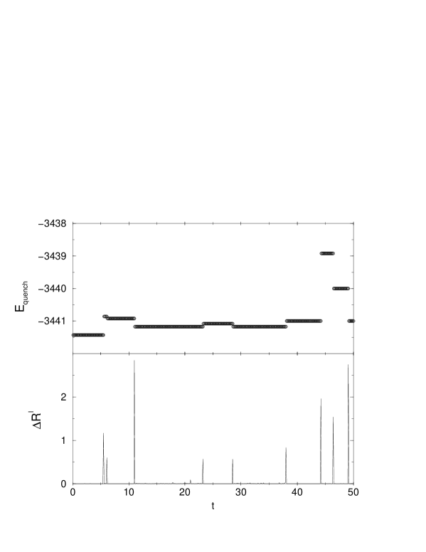
Figure 4.6: Identifying transition among inherent structures; a) $E_{quench}$ vs. time. b) $\Delta R^{I}$ (equation 4.3) vs. time. Transitions between (the basin of attraction of) inherent structures is indicated by a jump in $E_{quench}(t)$ and a corresponding peak in $\Delta R^{I}(t)$.

Each jump in $E_{quench}(t)$ is associated with a peak in $\Delta R^{I}(t)$, indicating the system has moved to a different inherent structure. A transition might in principle occur between two inherent structures with exactly the same (quenched) energy. Such a transition would not be seen in $E_{quench}(t)$, and consequently we use $\Delta R^{I}(t)$ to identify transitions. The distribution of $\log_{10}(\Delta R^{I}(t))$ is shown in figure 4.7. The distribution is seen to have two separated peaks. The peak to the left (centered around $\log_{10}(\Delta R^{I}(t))\approx{-3})$ is due to numerical uncertainties; two configurations within the same basin of attraction is not quenched to the exactly the same configuration. The peak on the right is the one containing the physically interesting transitions, which is seen to have $\Delta R^{I}$ on the order of unity. In the following we use the condition $\Delta R^{I}>0.1$ to identify the (physically interesting) transitions.

Figure 4.7: Distribution of $\log_{10}(\Delta R^{I}(t))$. This distribution is not normalized, i.e. the y-axes indicates how many quenches gave values of $\log_{10}(\Delta R^{I}(t))$ in the interval on the x-axis.

Figure 4.7 shows that most of the quenches results in not finding a transition (left peak), and only a small fraction results in actually finding a transition (right peak). Or in actual numbers: Doing 7500 quenches we found 440 transitions. The quenching procedure takes a considerable amount of time (corresponding to approximately 1000 MD steps), which is why we haven’t simply continued this procedure to find a larger number of transitions. The data presented in the following is averaged over the 440 transitions found using the “brute force” method described above, and should be considered preliminary. (NOTE: In paper III  results from 12000 transitions are reported. The results are similar to the results presented here, except of course with less noise).

For each transition, we monitor the displacements of the particles from one inherent structure to the other. The distribution of all particle displacements is shown in Fig. 4.8. While many particles move only a small distance ($r<0.2$) during the transition, a number of particles move farther, and in particular, we find that the distribution for $r>0.2$ is to a good approximation exponential. At present we have no explanation for this. The dotted curve is a fit to a power-law with exponent $-5/2$, which is a prediction from linear elasticity theory [70, 71], describing the displacements of particles in the surroundings of a local “event”. This power-law fit does not look very convincing by it self, but we note that the exponent was not treated as a fitting parameter (i.e. only the prefactor was fitted), and the power-law is expected to break down at small displacements, since these corresponds to distances far away from the local event, and is thus not seen in our finite sample. From the change in behavior of $p(r)$ at $r\approx 0.2$, it is reasonably to think of particles with displacements larger than $0.2$, as those taking part in the local event, and the rest of the particles as being in the surroundings, adjusting to the local event. Using this definition it is found that on average approximately 10 particles participate in an event.

Figure 4.8: Distribution of particle displacements during transitions between consecutive inherent structures at T=0.59. Full curve is a fit to an exponential, for $r>0.2$. The dotted curve is a fit to a power-law with exponent $-5/2$, as predicted by linear elasticity theory (see text).

Figure 4.8 has two important consequences with regards to points discussed earlier in this thesis; i) The distribution of particle displacements during transitions shows no preference for displacement of the average inter-particle distance ($\approx 1$ in the used units). This shows that the hopping indicated by the secondary peak in $4\pi r^{2}G_{s}(r,t)$ (figure 3.7 and 3.9) at low temperatures is not due to transitions over single energy barriers. A (correlated) sequence of the these is needed, to “build up” the secondary peak. This is consistent with the behavior seen in the inherent trajectory in figure 4.3; The jump does not happen in one step, but through a number of “intermediate” inherent structures. ii) Particles in the surroundings of a local event are displaced small distances, to adjust to the larger displacements occurring in the local region of the event itself. This kind of motion is very hard to detect in the true dynamics, since it is dominated by the thermal vibrations. Presumably this kind of motion is the reason why the inherent trajectory in figure 4.3 still retains some motion “within” the vibrations; as a consequence of an event in the surroundings, the particle starts vibrating around a position that is slightly displaced. This view of the dynamics is also consistent with the fact, that the first peak in $4\pi r^{2}G_{s}^{I}(r,t)$ is not a delta function in $r=0$ (see discussion in section 4.4).

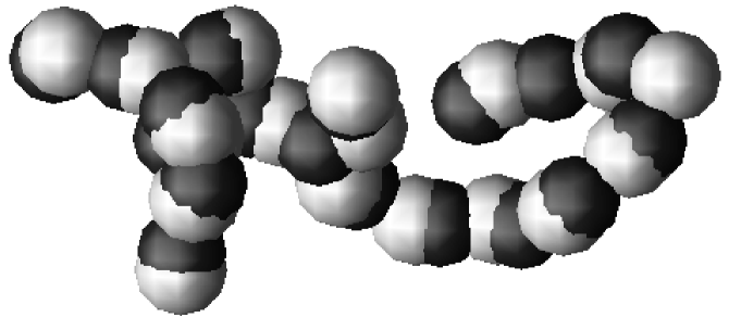
Figure 4.9: Before (light) and after (dark) one typical transition, all the particles which move a distance greater than 0.2. The cooperative, string-like nature of the particle motions during the inter-basin transition can be clearly seen.

From visual inspection of a number of the identified transitions it was found, that these are cooperative and string-like in nature. By visual inspection is here meant, that the position of particles moving more than $0.2$ during the transition, is plotted before and after the transition, see figure 4.9. String-like motion has been found to be an important part of the dynamics of glass-forming liquids. It is the natural consequence of particles hopping to positions previous occupied by other particles (as concluded from figure 3.10), and it was found (and quantified) in the Kob & Andersen system, when looking at the “mobile” particles [36]. In paper II strings was also found when looking at how particles was displaced (in the inherent structures) during the time interval $t^{*}$ (figure 3 in paper II). In paper II  this was described as “vacancy hopping”; one particle jumps, leaving room for another particle to jump, etc. The finding that also transitions over energy barriers are associated with strings, indicates that the vacancy hopping interpretation might not be correct; it seems to indicate that (at least some of) the strings are really cooperative in nature, i.e the particles in the string move at the same time. Further (quantitative) investigations are obviously needed to answer this question.

4.6 Conclusion

In this chapter we have presented results from analyzing the dynamics of a model glass-forming liquid in terms of its potential energy landscape. We did so by introducing the new concept of “inherent dynamics”, which can be thought of as a course-graining of the true dynamics, where the part of the dynamics related to vibrations around single inherent structures is removed.

Comparing the self intermediate scattering function, $F_{s}(q,t)$, with its inherent counterpart, $F_{s}^{I}(q,t)$, we found direct numerical evidence for the existence of a transition temperature, $T_{x}$, below which the true dynamics is separated into vibrations around inherent structures and transitions between these (the “vibrations plus transitions scenario”). We thus confirm the “energy landscape” picture, which is (at least) 30 years old. Given the fact the energy landscape does exist (since its simply the potential energy as function of the particle coordinates) and it does have a number of local minima (inherent structures), it is not surprising that the dynamics becomes dominated by the energy barriers at sufficiently low temperatures. What we have done here using the concept of inherent dynamics, is to provide direct numerical evidence for this, and we have shown that this regime can be reached by (pseudo-) equilibrium molecular dynamics (for the particular system investigated here). To our knowledge this is the first time such evidence has been presented.

The fact that we have been able to cool the system, under equilibrium conditions, to temperatures where the separation between vibrations around inherent structures and transitions between these is (almost) complete, means that it now makes sense to study the individual transitions over energy barriers, since these in this regime are “significant”. There is a lot of interesting questions to investigate regarding these transitions, and we have here only investigated a few of these. Specifically, we have not determined the energy barriers, but only compared the two inherent structures involved in a particular transition. This is an obvious point for further investigations.

Chapter 5 The Symmetric Hopping Model

The symmetric hopping model is introduced, and three analytical approximations for calculating the frequency dependent diffusion coefficient, $D(s)$, in the extreme disorder limit (low temperatures) of the model is described; the Effective Medium Approximation (EMA), the Percolation Path Approximation (PPA), and the Diffusion Cluster Approximation (DCA). DCA is a new approximation, developed by my supervisor Jeppe C. Dyre (See paper IV and V). Two numerical methods for calculating $D(s)$ in the extreme disorder limit is discussed. The first method is derived from the mean square displacement and is equivalent with the method of the ac Miller-Abrahams (ACMA) electrical equivalent circuit. The second method (VAC) is derived from the velocity auto correlation and is a new method. Numerical results using the VAC method are compared to the three analytical approximations, and previous results from the ACMA method.

The main results in this chapter are the development of the VAC method (section 5.5), and the numerical results it leads to (section 5.6 and 5.7). Results in this chapter are published in paper IV and V.

5.1 The Symmetric Hopping Model

The symmetric hopping model [23, 24, 25, 26, 27, 28] is defined in the following way: A particle ’lives’ on the sites of a $\mathcal{D}$-dimensional regular lattice (see figure 5.1 for a 1-dimensional illustration), where all the sites has the same energy (which we set to 0). The particle jumps over energy barriers connecting nearest neighbor sites, with jump rates (probability per unit time) given by $\Gamma(k\rightarrow i)=\Gamma_{0}\exp(-\beta E_{ki})$, where $\Gamma_{0}$ is the (constant) “attack-frequency”, $\beta\equiv(k_{B}T)^{-1}$ and $E_{ki}$ is the energy barrier between the two sites. The energy barriers are chosen randomly, from a probability distribution, $p(E)$, (to be specified). Jump rates between sites that are not nearest neighbors are zero. It follows from the above, that $\Gamma(i\rightarrow k)=\Gamma(k\rightarrow i)$, i.e. the jump-rates are symmetric. In the following we will use $\Gamma(E)\equiv\Gamma_{0}\exp(-\beta E)$, and denote the lattice constant $a$.

Figure 5.1: The symmetric hopping model in 1 dimension. A particle jumps between nearest neighbor sites, by crossing energy barriers connecting these. The jump-rates are given by $\Gamma(i\rightarrow i+1)=\Gamma_{0}\exp(-\beta E_{i,i+1})$, where $E_{i,i+1}$ is the energy barrier between the two sites.

If all the energy barriers are identical, i.e. $p(E)=\delta(E-E_{0})$, the model describes diffusion in an ordered structure, and one finds normal diffusive behavior:

$$\langle{\Delta X}^{2}(t)\rangle=2Dt$$ (5.1)

where $\langle{\Delta X}^{2}(t)\rangle$ is the mean square displacement along the x-direction, and $D=a^{2}\Gamma(E_{0})$ is the diffusion coefficient [25]. The average in equation 5.1 can either be a time-average or a ensemble average. We will in the following use the ensemble average, which is characterized by all the sites having the same probability (since they have the same energy). Instead of ensembles it is convenient to think of a (large) number of independent particles moving around in the sample.

In a sample where the energy barriers are not identical, equation 5.1 does not hold at all time scales. Picture for example a 1-dimensional sample with mostly small energy barriers, $E_{small}$, and a few much larger energy barriers, $E_{large}$, (see eg. [72]). At small time scales most of the particles will “think” they are living on an ordered sample with only the small energy barriers (since they haven’t yet encountered a large energy barrier), and the ensemble will follow equation 5.1 with a large diffusion coefficient ($\propto\Gamma(E_{small})$). However, at long time scales the particles will start to “feel” the effect of the large energy barriers, which will slow down the diffusion. At very long time and length scales the sample will appear homogeneous and the system again become diffusive, but now with a small diffusion coefficient ($\propto\Gamma(E_{large})$).

The deviations from equation 5.1 can be quantified using the time dependent diffusion coefficient [73], $D(t)$, or the frequency dependent diffusion coefficient [74], $D(s)$ (with $s$ being the Laplace frequency, $s=i\omega$):

$$D(t) = \frac{1}{2}\frac{d}{dt}\langle{\Delta X}^{2}(t)\rangle$$ (5.2)

$$D(s) = s\int_{0}^{\infty}e^{-st}D(t)dt=\frac{s^{2}}{2}\int_{0}^{\infty}e^{-st}\langle{\Delta X}^{2}(t)\rangle dt$$ (5.3)

Note, that for diffusion in a sample with identical energy barriers, equation 5.1 leads to $D(s)=D(t)=D$.

In a disordered sample one in general finds that the system becomes diffusive at long time scales (corresponding to low frequencies) when particles are moving much longer than the appropriate correlation length (assuming that such a correlation length exists); $D_{0}\equiv D(s\rightarrow 0)=D(t\rightarrow\infty)$. In one dimension one finds [75]: $D_{0}=a^{2}\langle\Gamma^{-1}\rangle^{-1}$, where the average is over the distribution of jump rates, $\Gamma$. In higher dimensions no such simple expression exists, but for $\beta\rightarrow\infty$ one finds [76]: $D_{0}\propto\Gamma(E_{c})$, where $E_{c}$ is the so-called percolation energy (see section 5.3.2).

At infinitely short time particles never jumps more than once, and one finds (where $\Gamma_{L}$ and $\Gamma_{R}$ are respectively the jump rates to the left and to the right of a given site):

$$\langle{\Delta X}^{2}(\Delta t)\rangle = \langle a^{2}\Gamma_{L}\Delta t+a^{2}\Gamma_{R}\Delta t\rangle$$ (5.4)

$$= 2a^{2}\langle\Gamma\rangle\Delta t$$ (5.5)

In the high-frequency limit, we thus find: $D_{\infty}\equiv D(s\rightarrow\infty)=D(t\rightarrow 0)=a^{2}\langle\Gamma\rangle$.

In [25] and paper I, the symmetric hopping model was treated as a model for frequency dependent conduction in glasses. In that context the particles represent non-interacting charge carriers (ions or electrons), and the lattice sites represents the positions in the glass where the charge carriers can reside. The frequency dependent conductivity, $\sigma(s)$, is related to $D(s)$ by the generalized Einstein relation [74]:

$$\sigma(s)=\frac{e^{2}n}{k_{B}T}D(s)$$ (5.6)

where $n$ is the density of particles, and $e$ is the charge of the particles.

In the present work we shift the attention slightly, and treat the symmetric hopping model more generally as a model for diffusion in disordered media. We focus on the “extreme disorder limit”, i.e. low temperatures, where the model is found to exhibit universal behavior; $D(s)$ becomes independent (suitably scaled) of the temperature and the chosen probability distribution for the energy barriers, $p(E)$. In the extreme disorder limit, it is not feasible to simulate the model using standard Monte Carlo (MC) techniques [24, 26, 77]; Due to the large difference in jump rates ($\propto e^{-\beta E}$), the particle will jump many times over small energy barriers, and only “sample” the rest of the lattice on much larger time scales. Although this reflects the physics of the model in the extreme disorder limit, it makes MC methods unsuitable in this limit.

In the following we set the attack frequency, $\Gamma_{0}=1$, the lattice constant, $a=1$, and Boltzmann’s constant, $k_{B}=1$, thus defining the scales for time, length, and energy respectively.

5.2 The Master Equation

The starting point for both the analytical and the numerical methods, is the master equation [78, 79, 80, 81, 82] for the model; Let $P(i,t|j,0)$ denote the probability of the particle being at site $i$ at time $t$, given that it was at site $j$ at $t=0$. The master equation for the system is then:

$$\frac{dP(i,t|j,0)}{dt}=-\gamma_{i}P(i,t|j,0)+\sum_{k}\Gamma(k\rightarrow i)P(k,t|j,0)$$ (5.7)

where $\gamma_{i}\equiv\sum_{k}\Gamma(i\rightarrow k)$. The first term on the right hand side is the probability flow out of site $i$, and the second term is the flow into site $i$. Defining the ($N^{\mathcal{D}}$x$N^{\mathcal{D}}$) matrix $\mathbf{P}(t)$ with the components $\mathbf{P}_{ij}(t)=P(i,t|j,0)$, we write the master equation on matrix form:

$$\frac{d}{dt}{\mathbf{P}}(t)={\mathbf{HP}}(t)$$ (5.8)

$\mathbf{H}$ is here a ($N^{\mathcal{D}}$x$N^{\mathcal{D}}$) matrix containing the jump rates; $\mathbf{H}_{ii}=-\gamma_{i}$ and $\mathbf{H}_{i\neq k}=\Gamma(k\rightarrow i)$. Note that only $2\mathcal{D}+1$ elements in each row in $\mathbf{H}$ are different from zero (the diagonal and the $2\mathcal{D}$ elements corresponding to nearest neighbors); $\mathbf{H}$ is sparse. This is an essential feature in the numerical methods; without it we wouldn’t be able to treat large enough sample sizes.

Taking the Laplace transform of equation 5.8 we get:

$$s{\mathbf{G}}(s)-\mathbf{P}(t=0)={\mathbf{HG}}(s)$$ (5.9)

where the $\mathbf{G}_{ij}(s)$ is the Green’s function, i.e. the Laplace transform of $\mathbf{P}_{ij}(t)$: $\mathbf{G}_{ij}(s)\equiv\int_{0}^{\infty}\mathbf{P}_{ij}(t)e^{-st}dt$. The initial condition, $\mathbf{P}(t=0)$, is given by the identity matrix, $\mathbf{I}$, and we thus find:

$$(s\mathbf{I}-\mathbf{H}){\mathbf{G}}(s)=\mathbf{I}~{}~{}~{}\Leftrightarrow~{}~{}~{}{\mathbf{G}}(s)=(s\mathbf{I}-\mathbf{H})^{-1}$$ (5.10)

Before proceeding to discuss the analytical approximations and the numerical methods, we present a “preview” of the dynamics of the symmetric hopping model in figure 5.2. A 2 dimensional sample was set up using a box-distribution of barrier energies; $p(E)=1,0\leq E\leq 1$. The time evolution of ${\mathbf{P}}(t)$ was determined by a discrete version of the master equation (eq. 5.8):

$${\mathbf{P}}(t+\Delta t)~{}=~{}{\mathbf{P}}(t)+\Delta t{\mathbf{HP}}(t)~{}=~{}({\mathbf{I}}+\Delta t{\mathbf{H}}){\mathbf{P}}(t)$$ (5.11)

A time step of $\Delta t=0.1$ was used, and as initial condition a particle was placed at a particular site. In figure 5.2a ${\mathbf{P}}(t=2)$ is shown for $\beta=0$, i.e. infinitely high temperature. In this limit all the jump rates are identical (equal to unity), and as expected the probability distribution spreads in a symmetric manner. In figure 5.2b ${\mathbf{P}}(t=10^{5})$ is shown for $\beta=40$, with the same starting position, and same energy landscape (i.e. same set of energy barriers) as in figure 5.2a. The time at which the two temperatures are compared was chosen so that the probability of finding the particle at the starting point was the same ($\approx 0.04$). The qualitative difference between the dynamics at high and low temperature is evident; At the low temperature (figure 5.2b) the spread of the probability distribution ${\mathbf{P}}(t)$ is highly irregular, as a consequence of the particles “preferring” low energy barriers and avoiding high energy-barriers. The particular structure of ${\mathbf{P}}(t)$ at the low temperature depends strongly on where the particle was started. If it was started in one of the two enclosed empty sites (white in figure 5.2b) it would be stuck there on the time scale used here, since these must be connected with high energy-barriers to the surroundings (otherwise they would not be empty in figure 5.2b).

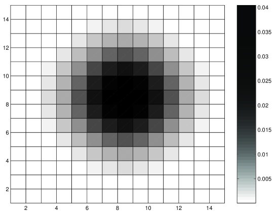
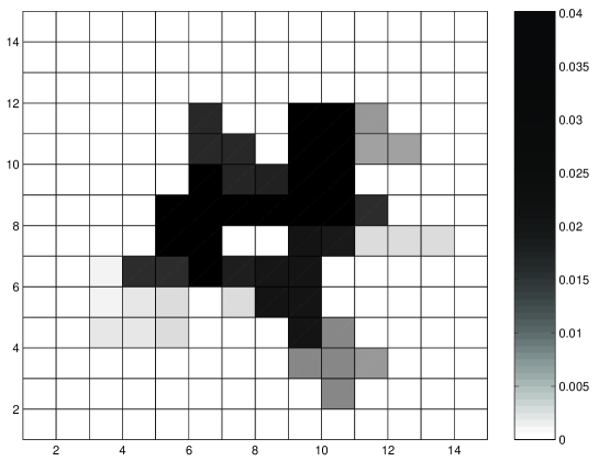
Figure 5.2: ${\mathbf{P}}(t)$ for a 2 dimensional realization of the symmetric hopping model, with a box distribution of energy-barriers. Each site is represented by a square, and this is colored a shade of grey according to the value of ${\mathbf{P}}(t)$ at the given site. a) ${\mathbf{P}}(t=2)$ for $\beta=0$. b) ${\mathbf{P}}(t=10^{5})$ for $\beta=40$.

5.3 Analytical approximations

In this section we’ll briefly describe the 3 analytical approximations which will be compared to the numerical results, in section 5.6 and 5.7.

5.3.1 Effective Medium Approximation (EMA)

In EMA [80, 25] the disordered sample is replaced by an ordered sample (the “effective medium”), where all the jump rates are replaced by an “effective” jump-rate, $\Gamma_{E}(s)$. The value of $\Gamma_{E}(s)$ is determined by a self-consistency condition; A single jump rate in the effective medium is replaced by its value in the disordered sample, and an average is performed over the distribution of jump rates. The condition that this average should be equivalent with the effective medium leads to the following condition [80, 25, 32]:

$$\left<\frac{D-\Gamma}{\mathcal{D}D-(D-\Gamma)(1-s\tilde{G})}\right>_{\Gamma} = 0$$ (5.12)

where $\tilde{G}$ is the diagonal element of the Green’s function for the effective medium, which depends on the spatial dimension, $\mathcal{D}$. In the extreme disorder limit ($\beta\rightarrow\infty$) one finds [25] for $\mathcal{D}\geq 2$:

$$\tilde{D}\ln(\tilde{D})=\tilde{s}$$ (5.13)

where $\tilde{D}\equiv D(s)/D_{0}$, and $\tilde{s}\equiv s/s_{c}$, where $s_{c}$ is a suitably defined characteristic frequency. The EMA thus predicts universality in the extreme disorder limit; Properly scaled $D(s)$ becomes independent of temperature and the distribution of energy barriers, $p(E)$.

In [25] the predictions of EMA was compared with numerical results using the ACMA method (described in section 5.4) in 2 dimensions. The existence of universality was confirmed by the numerical results (for 4 different energy-distributions), but the shape of $\tilde{D}(\tilde{s})$ was found to deviate from the one predicted by EMA. Or to be more specific: EMA predicts a shape of the universal $\tilde{D}(\tilde{s})$ that is growing to rapidly at the onset of frequency dependence; it is to “sharp” (figure 5 in [25]). The EMA prediction for $\langle{\Delta X}^{2}(t)\rangle$ is discussed in [83].

5.3.2 Percolation Path Approximation (PPA)

In the extreme disorder limit, the low-frequency diffusion is expected to be dominated by percolation [82, 84, 85, 77]; when diffusing over long distances (i.e. in the low-frequency limit) the particles “chose” to do so by jumping over energy-barriers that are as small as possible. The largest energy barrier that a particle has to cross to move through the sample is given by the “percolation energy”, $E_{c}$, defined by [25]:

$$\int_{0}^{E_{c}}p(E)dE=p_{c}$$ (5.14)

where $p_{c}$ is the percolation threshold for bond percolation (for an introduction to percolation theory, see [86]). In a 2 dimensional regular lattice $p_{c}$ equals $1/2$ (exact) and in a 3 dimensional cubic sample $p_{c}$ equals $0.2488$ (approximated). Equation 5.14 can be interpreted as follows; In a given sample mark the energy-barriers (bonds) starting with the smallest energy-barrier, then the next smallest etc. At some point the marked energy-barriers will “percolate” i.e. make a cluster that stretches through the whole sample (the “percolation cluster”). The highest energy needed to get percolation is (for an infinite sample) $E_{c}$. For the box distribution of energy barriers used in the present work ($p(E)=1,0\leq E\leq 1$), the percolation energy equals the (bond) percolation threshold: $E_{c}=p_{c}$. The percolation cluster is a fractal, with fractal dimension 1.9 and 2.5 in 2 and 3 dimensions respectively [86].

In paper I we argue, that the reason why EMA does not predict the shape of the universal curve $\tilde{D}(\tilde{s})$ in the extreme disorder limit correctly might be, that it replaces the disordered sample by an effective media of the same dimension, whereas the actual low frequency diffusion happens on a cluster of lower dimensionality. We will here term this cluster “the diffusion cluster”, and its fractal dimension $D_{f}$ (this is not the same as the percolation cluster, see below). PPA can be considered as a first attempt at trying to incorporate the fractal dimension of the diffusion cluster into an analytical approximation.

The percolation cluster contain “dead-ends”, which contributes little to the low frequency diffusion. Removing dead-ends from the percolation cluster leaves us with the “backbone”, with fractal dimension 1.6 and 1.7 in 2 and 3 dimensions respectively [86]. In paper I we argue, that $D_{f}$ is even lower, since the backbone contains loops, where one of the branches usually will be preferred (since the jump-rates depend strongly on the energy barriers in the extreme disorder limit). In PPA the extreme view that $D_{f}=1$ is taken, i.e. that the (low frequency) diffusion takes place on 1-dimensional “percolation paths”. With this assumption we in paper I arrive at the PPA approximation, given by:

$$\sqrt{\tilde{s}\tilde{D}}\ln\left(1+\sqrt{\tilde{s}\tilde{D}}\right)=\tilde{s}$$ (5.15)

PPA thus predicts universality in the extreme disorder limit, like is the case for EMA. In paper I , we find that PPA agrees better with the numerical results than EMA. This is especially true in 3 dimensions. The agreement is however not perfect, and a number of problems remain unanswered (see last section in paper I). The PPA prediction for $\langle{\Delta X}^{2}(t)\rangle$ is discussed in [87].

5.3.3 The Diffusion Cluster Approximation (DCA)

The Diffusion Cluster Approximation can be thought of as a refinement of PPA (paper IV and V); instead of setting $D_{f}=1$, this is in DCA left as a parameter in the model. Using the approach of EMA, but with an fractal effective medium with fractal dimension $D_{f}$, one finds:

$$\ln(\tilde{D})=\left(\frac{\tilde{s}}{\tilde{D}}\right)^{{D_{f}}/{2}}$$ (5.16)

This expression is limited to $1<D_{f}<2$. For $D_{f}\geq 2$ DCA reduces to the EMA prediction (eq. 5.13), and for $D_{f}\leq 1$ it is undefined. Since we do not have an independent estimate of $D_{f}$ we will in the present work treat it as a fitting parameter. This must obviously be taken into consideration, when comparing with EMA and PPA, since these have no fitting parameters.

From the arguments given above, we expect $D_{f}$ to be limited above by the fractal dimension of the backbone. Furthermore we expect $D_{f}$ to limited below by the fractal dimension of the so-called “red bonds”, which are the singly connected bonds on the backbone, i.e. if a red bond is removed the backbone is broken into 2 parts. The fractal dimension of the red bonds are $3/4$ and $1.14$ in 2 and 3 dimensions respectively.

5.4 The ACMA Method

In this section we briefly describe the ACMA method, which was used to obtain the numerical results reported in [25] and paper I.

Defining $X_{i}$ as the x-coordinate of site $i$ we can write the frequency dependent diffusion coefficient (equation 5.3):

$$D_{x}(s) = \frac{s^{2}}{2}\int_{0}^{\infty}e^{-st}\frac{1}{N^{d}}\sum_{i,j}(X_{i}-X_{j})^{2}\langle P(i,t|j,0)\rangle dt$$ (5.17)

$$= \frac{s^{2}}{2N^{d}}\sum_{i,j}(X_{i}-X_{j})^{2}\langle G(i,s|j)\rangle$$ (5.18)

The subscript $x$ in $D_{x}(s)$ is here used to emphasize that the diffusion coefficient here is calculated from the mean square displacement in the x-direction. In more than 1 dimension similar expressions obviously hold for other directions.

Equation 5.10 and equation 5.18 together constitutes a method for computing D(s); calculate $\langle G(i,s|j)\rangle$ by inverting $(s\mathbf{I}-\mathbf{H})$ (equation 5.10) and insert the result in equation 5.18 [74].

Figure 5.3: The ac Miller-Abrahams (ACMA) electrical equivalent circuit for the symmetric hopping model. The admittance of the resistor between two sites is equal to the corresponding jump rate. The admittance of the capacitors are $s$.

In my master thesis [32, 33] it was demonstrated, that the method described above is equivalent to the method of the ac Miller-Abrahams (ACMA) electrical equivalent circuit [25]. In this method a large network of linear electric components are set up (see figure 5.3 for an illustration of the 1-dimensional case). After eliminating all the ’internal sites’ (those without numbers in figure 5.3) by the so-called generalized Star-Mesh transformation, $\sigma(s)$ ($\propto D(s)$, see equation 5.6) is calculated as a weighted sum over the effective conductances between the ’external sites’ (those with numbers in figure 5.3). The elimination process described above is equivalent with Gauss-Jordan elimination on the matrix $(s\mathbf{I}-\mathbf{H})$ [33], and the Fogelholm algorithm [88] for the order in which the internal sites are eliminated is equivalent with the minimum degree pivoting algorithm [89]: At each step eliminate the site/row with the smallest number of connections/elements.

A number of ’tricks’ is used in the ACMA method, to improve efficiency over a straight forward computation of first equation 5.10 and then equation 5.18. The most important trick is that the (dense) matrix $\mathbf{G}(s)$ is not explicitly calculated, but instead a ’condensed’ version where columns corresponding to the sites with the same x-coordinate are added together. Thus instead of solving for $N^{\mathcal{D}}$ right-hand sides (inverting $s\mathbf{I}-\mathbf{H}$) only $N$ right-hand sides are used.

In the simulations using the ACMA method presented in [25] and paper I ’perfect electrodes’ were used in the x-direction (see figure 5.3). This ensures that $D(s)$ goes to a constant value as $s\rightarrow 0$, corresponding to $\langle{\Delta X}^{2}(t)\rangle$ being proportional to $t$, as $t\rightarrow\infty$, i.e. the system being diffusive. However, with this modification the model does not correspond directly to the solution of a master equation. This is evident from the fact that the mean square displacement as calculated in equation 5.17 is finite for any finite sample, and thus it can not be proportional to $t$ at long times.

To what extent the ’perfect electrodes’ mimics the effect of real electrodes when experimentally measuring the frequency dependent conductivity, $\sigma(s)$, will not be discussed here. What we are after here, is to calculate the bulk value of the frequency dependent diffusion coefficient $D(s)$ in the extreme disorder limit.

5.5 The Velocity Auto Correlation (VAC) method

In this section the Velocity Auto Correlation (VAC) method is developed. Its main advantages over the ACMA method is, that it can be (and is) used with periodic boundary conditions, and still give a diffusive regime for $s\rightarrow 0$ (i.e. $t\rightarrow\infty$). Another advantage over the ACMA method (as it was implemented in the previous work), is that the VAC method is formulated in terms of sparse matrices, which means that standard methods for solving these can be used. The differences between the two methods will be discussed further in section 5.8.

To derive the VAC method we express the diffusion coefficient in terms of the velocity auto correlation function [74]:

$$D_{x}(s)=\int_{0}^{\infty}\left<v(t)v(0)\right>_{x}e^{-st}dt$$ (5.19)

$v(t)$ is here the velocity (in the x-direction) of the particle at time t. The motion of the particle in the symmetric hopping model is instantaneous; when it jumps from one site to another, this happens in a infinitesimally small time-interval, $\Delta t$. We may thus assign the constant velocity $\pm a/\Delta t$ (where we briefly reintroduce the lattice constant, $a$) to the particle in the time interval, $\Delta t$, ensuring that it moves one lattice constant, $a$, either to the left or to the right. $v(t)$ thus takes on the value $a/\Delta t$ in a time interval $\Delta t$ when the particle jumps to the right, the value $-a/\Delta t$ in a time interval $\Delta t$ when the particle jumps to the left, and zero the rest of the time (It is not important whether or not this is a physically reasonable choice for $v(t)$. The only requirement for eq. 5.19 to hold is that $x(t)=\int_{o}^{t}v(t)dt+x(o)$). With this choice of $v(t)$, the function $v(t^{\prime})v(0)$ has the value $a^{2}/\Delta t^{2}$ if the particle jumps in the same direction at $t=t^{\prime}$ and $t=0$, the value $-a^{2}/\Delta t^{2}$ if the particle jumps in opposite directions at $t=t^{\prime}$ and $t=0$, and zero otherwise (i.e if the particle does not jump both at $t=t^{\prime}$ and $t=0$).

The probability, $P_{RR}$, that the particle jumps to the right both at $t=t^{\prime}$ and $t=0$ is (for now we assume that $t^{\prime}\neq 0$):

$$P_{RR} = \frac{1}{N^{d}}\sum_{i,j}\Gamma_{R}(j)\Delta t\left<P(i,t|j+1,0)\right>\Gamma_{R}(i)\Delta t$$ (5.20)

$$= \frac{\Delta t^{2}}{N^{d}}\sum_{i,j}\Gamma_{L}(j)\left<P(i,t|j,0)\right>\Gamma_{R}(i)$$ (5.21)

Equation 5.20 can be read from the left as follows; If the particle starts at site $j$ the probability of jumping to the right at $t=0$ is $\Gamma_{R}(j)\Delta t$. This means that it is now at site $j+1$, and the probability that it moves to site $i$ in the time $t$ is $\left<P(i,t|j+1,0)\right>$, and finally the probability that it jumps to the right from site $i$ is $\Gamma_{R}(i)\Delta t$. In equation 5.21 $j$ is substituted with $j-1$, and $\Gamma_{R}(j-1)=\Gamma_{L}(j)$ is used. Calculating in the same way the probability of the other events that contributes to the velocity auto correlation function, $\left<v(t)v(0)\right>_{x}$ ($P_{RL}$, $P_{LR}$, and $P_{LL}$), we can now write $\left<v(t)v(0)\right>_{x}$, in terms of the Green’s function (where again use $a=1$, and the delta function takes care of the special case $t=0$, see below):

$$\left<v(t)v(0)\right>_{x} = C\delta(t)+\frac{1}{\Delta t^{2}}\sum_{i,j}(P_{RR}+P_{LL}-P_{RL}-P_{LR})$$ (5.22)

$$= C\delta(t)+\frac{1}{N^{d}}\sum_{i,j}\left<P(i,t|j,0)\right>$$

$$\left[\Gamma_{L}(j)\Gamma_{R}(i)+\Gamma_{R}(j)\Gamma_{L}(i)-\Gamma_{L}(j)\Gamma_{L}(i)-\Gamma_{R}(j)\Gamma_{R}(i)\right]_{~{}}$$

$$= C\delta(t)^{~{}}+$$

$$\frac{1}{N^{d}}\sum_{i,j}(\Gamma_{R}(i)-\Gamma_{L}(i))\left<P(i,t|j,0)\right>(\Gamma_{L}(j)-\Gamma_{R}(j))$$

Taking the Laplace transform of equation 5.5 we get:

$$D_{x}(s)=C+\frac{1}{N^{d}}\sum_{i,j}(\Gamma_{R}(i)-\Gamma_{L}(i))\left<G(i,s|j)\right>(\Gamma_{L}(j)-\Gamma_{R}(j))$$ (5.25)

In the high- frequency limit, $s\rightarrow\infty$, we find from equation 5.10
$\left<G(i,s|j)\right>\rightarrow 0$. We thus get $C=D_{\infty}=\left<\Gamma\right>$ (see equation 5.5):

$$D_{x}(s)=\left<\Gamma\right>-\frac{1}{N^{d}}\sum_{i,j}(\Gamma_{R}(i)-\Gamma_{L}(i))\left<G(i,s|j)\right>(\Gamma_{R}(j)-\Gamma_{L}(j))$$ (5.26)

In the case where all the jump-rates are identical, $\Gamma_{R}(i)=\Gamma_{L}(i)$, equation 5.26 leads to $D_{x}(s)=\left<\Gamma\right>=D_{\infty}$, as expected (see section 5.1).

Equation 5.26 can be used together with equation 5.10 to calculate $D_{x}(s)$. However this method poses a serious numerical problem at low temperatures where $D_{0}$ is very small compared to $D_{\infty}$. Calculating $D_{x}(s)$ at low frequencies from equation 5.26 in this limit amounts to calculating a small difference between two large numbers, which leads to large uncertainties in the result.

In the following we will derive a version of the VAC method, which does not have the numerical problems described above. We do this first in 1 dimension (section 5.5.1), followed by a general derivation in $\mathcal{D}$ dimensions (section 5.5.2).

5.5.1 The VAC method in 1 Dimension

The idea behind the derivation of the VAC method in 1 dimension is to rewrite the problem in terms of the variable:

$$J_{R}(i,t|j,0)\equiv\Gamma_{R}(i)\left[P(i,t|j,0)-P(i+1,t|j,0)\right]$$ (5.27)

which can be interpreted as the particle current to the right of site $i$ at time $t$ given that the particle started at site $j$ at $t=0$. The master equation (5.7) can then be written as:

$$\frac{dP(i,t|j,0)}{dt}=J_{R}(i-1,t|j,0)-J_{R}(i,t|j,0)$$ (5.28)

We now define two new matrices; $\mathbf{\Gamma}_{R}$ is a diagonal matrix containing the jump rates to the right of each site: $(\mathbf{\Gamma}_{R})_{ij}=\delta(i,j)\Gamma_{R}(i)$. $\mathbf{A}$ is a matrix with $+1$ on the diagonal, $-1$ on the sub-diagonal and zero everywhere else: $(\mathbf{A})_{ij}=\delta(i,j)-\delta(i-1,j)$. In more general terms; $\mathbf{A}_{ij}$ equals $-1$ if site $j$ is the left neighbor to site $i$. Here (as in the rest of this chapter) periodic boundary conditions are implicit, i.e. $(\mathbf{A})_{1N}=-1$. We can now write the 1 dimensional master equation as:

$$\frac{d}{dt}\mathbf{P}(t) = -\mathbf{A}\mathbf{J}_{R}(t),~{}~{}~{}\mathbf{J}_{R}(t)=\mathbf{\Gamma}_{R}\mathbf{A}^{T}\mathbf{P}(t)$$ (5.29)

These equations provides us with an an explicit expression for the matrix $\mathbf{H}$ in the master equation (5.8): $\mathbf{H}=-\mathbf{A}\mathbf{\Gamma}_{R}\mathbf{A}^{T}$. What we are after here is however an equation for $\mathbf{J}_{R}$. To get this we take the Laplace transform of equation 5.29:

$$s\mathbf{G}(s)+\mathbf{A}\mathbf{J}_{R}(s)=\mathbf{P}(t=0)=\mathbf{I}$$ (5.30)

where $\mathbf{J}_{R}(s)$ is the Laplace transform of $\mathbf{J}_{R}(t)$. By multiplying from the left by $\mathbf{A}^{T}$ and using $\mathbf{J}_{R}(s)=\mathbf{\Gamma}_{R}\mathbf{A}^{T}\mathbf{G}(s)$ we get:

$$(s\mathbf{\Gamma}_{R}^{-1}+\mathbf{A}^{T}\mathbf{A})\mathbf{J}_{R}(s)=\mathbf{A}^{T}\Leftrightarrow$$ (5.31)

$$\mathbf{J}_{R}(s)=(s\mathbf{\Gamma}_{R}^{-1}+\mathbf{A}^{T}\mathbf{A})^{-1}\mathbf{A}^{T}$$ (5.32)

Here we assume that the diagonal matrix $\mathbf{\Gamma}_{R}$ is invertible, i.e. that all the jump rates are different from zero. We are now ready to derive an equation for D(s) in 1 dimension. To do this we rewrite equation 5.26 using $\Gamma_{L}(i)=\Gamma_{R}(i-1)$:

$$D(s)=\left<\Gamma_{R}\right>-\frac{1}{N}\sum_{i,j}(\Gamma_{R}(i)-\Gamma_{R}(i-1))\left<G(i,s|j)\right>(\Gamma_{R}(j)-\Gamma_{R}(j-1))$$

This can be written as (where $\mathbf{1}$ is a column vector containing all 1’s):

$$D(s)N = \mathbf{1}^{T}\mathbf{\Gamma}_{R}\mathbf{1}-\mathbf{1}^{T}\mathbf{\Gamma}_{R}\mathbf{A}^{T}\mathbf{G}(s)\mathbf{A}\mathbf{\Gamma}_{R}\mathbf{1}$$ (5.33)

$$= \mathbf{1}^{T}\mathbf{\Gamma}_{R}\mathbf{1}-\mathbf{1}^{T}\mathbf{J}_{R}(s)\mathbf{A}\mathbf{\Gamma}_{R}\mathbf{1}$$ (5.34)

$$= \mathbf{1}^{T}\mathbf{\Gamma}_{R}\mathbf{1}-\mathbf{1}^{T}(s\mathbf{\Gamma}_{R}^{-1}+\mathbf{A}^{T}\mathbf{A})^{-1}\mathbf{A}^{T}\mathbf{A}\mathbf{\Gamma}_{R}\mathbf{1}$$

$$= \mathbf{1}^{T}(s\mathbf{\Gamma}_{R}^{-1}+\mathbf{A}^{T}\mathbf{A})^{-1}\left[(s\mathbf{\Gamma}_{R}^{-1}+\mathbf{A}^{T}\mathbf{A})-\mathbf{A}^{T}\mathbf{A}\right]\mathbf{\Gamma}_{R}\mathbf{1}$$

$$= s\mathbf{1}^{T}(s\mathbf{\Gamma}_{R}^{-1}+\mathbf{A}^{T}\mathbf{A})^{-1}\mathbf{1}$$ (5.36)

$$= s\mathbf{1}^{T}\mathbf{x},~{}~{}~{}(s\mathbf{\Gamma}_{R}^{-1}+\mathbf{A}^{T}\mathbf{A})\mathbf{x}=\mathbf{1}$$ (5.37)

We have now avoided the problematic subtraction (in equation 5.26 and 5.33), and reduced the problem to finding the vector $\mathbf{x}$ by solving a sparse system of linear equations.

5.5.2 The VAC method in $\mathcal{D}$ Dimensions

In this section we generalize the VAC method to $\mathcal{D}$ dimensions. In analogy with $\mathbf{J}_{R}(t)$ used in the 1-dimensional version, we define $\mathbf{J}_{k}(t)$ as the particle current in the $k$’th direction:

$$\mathbf{J}_{k}(t)=\mathbf{\Gamma}_{k}\mathbf{H}_{k}^{T}\mathbf{P}(t)$$ (5.38)

where $\mathbf{\Gamma}_{k}$ and $\mathbf{H}_{k}$ are generalization of the matrices $\mathbf{\Gamma}_{R}$ and $\mathbf{A}$ used in the previous section. $\mathbf{\Gamma}_{k}$ is a diagonal matrix, which for each site contains the jump rate to the “right” in the $k$’th direction. $(\mathbf{H}_{k})_{ij}$ equals $-1$ if site $j$ is the “left” neighbor to site $i$ along direction $k$, and it has $1$ on the diagonal and zero everywhere else. The structure of $\mathbf{H}_{k}$ depends on the numbering scheme chosen for the sites, but the resulting physics is obviously independent of this. An explicit expression for $\mathbf{H}_{k}$ (and the corresponding numbering of the sites) is given in appendix A.

The goal is now to set up a master-equation for the currents, and from that calculate $D(s)$, like it was done in the 1-dimensional case. Obviously it is not possible to solve for $\mathbf{J}_{k}(s)$ without at the same time solving for the currents in the other directions. We thus generalize equation 5.38 to

$$\mathbf{J}_{*}(t)=\mathbf{\Gamma}_{*}\mathbf{H}_{*}^{T}\mathbf{P}(t)~{}~{}\Leftrightarrow~{}~{}\mathbf{J}_{*}(s)=\mathbf{\Gamma}_{*}\mathbf{H}_{*}^{T}\mathbf{G}(s)$$ (5.39)

where we have defined the following block-matrices:

$$\mathbf{J}_{*}(t)\equiv\left(\begin{array}[]{c}\mathbf{J}_{1}(t)\\ \mathbf{J}_{2}(t)\\ \vdots\\ \mathbf{J}_{\mathcal{D}}(t)\\ \end{array}\right),~{}\mathbf{\Gamma}_{*}\!\!\! \equiv \!\!\!\left(\begin{array}[]{c c c c}\mathbf{\Gamma}_{1}&\mathbf{0}&&\mathbf{0}\\ \mathbf{0}&\mathbf{\Gamma}_{2}&&\mathbf{0}\\ &&\ddots&\\ \mathbf{0}&\mathbf{0}&&\mathbf{\Gamma}_{\mathcal{D}}\\ \end{array}\right),~{}\mathbf{H}_{*}\equiv\left(\mathbf{H}_{1},\dots,\mathbf{H}_{\mathcal{D}}\right)$$ (5.48)

and $\mathbf{J}_{*}(s)$ is the Laplace transform of $\mathbf{J}_{*}(t)$.

The master equation for $\mathbf{P}(t)$ is similar to the one in 1-dimension (eq. 5.29), but the change in the probability at a given site now has contributions from all $\mathcal{D}$ directions:

$$\frac{d}{dt}\mathbf{P}(t)=-\sum_{k=1}^{\mathcal{D}}\mathbf{H}_{k}\mathbf{J}_{k}(t)=-\mathbf{H}_{*}\mathbf{J}_{*}(t)=-\mathbf{H}_{*}\mathbf{\Gamma}_{*}\mathbf{H}_{*}^{T}\mathbf{P}(t)~{}~{}\Leftrightarrow~{}~{}~{}~{}~{}{}$$ (5.50)

$$s\mathbf{G}(s)+\mathbf{H}_{*}\mathbf{J}_{*}(s)=\mathbf{P}(t=0)$$ (5.51)

By multiplying equation 5.51 from the left with $\mathbf{\Gamma}_{*}\mathbf{H}_{*}^{T}$, and substituting for $\mathbf{J}_{*}(s)$ (equation 5.39), we arrive at the (Laplace transformed) master equation for $\mathbf{J}_{*}(s)$:

$$\left(s\mathbf{I}+\mathbf{\Gamma}_{*}\mathbf{H}_{*}^{T}\mathbf{H}_{*}\right)\mathbf{J}_{*}(s)=\mathbf{\Gamma}_{*}\mathbf{H}_{*}^{T}\mathbf{P}(t=0)~{}~{}\Leftrightarrow~{}~{}$$ (5.52)

$$\mathbf{J}_{*}(s)=\left(s\mathbf{I}+\mathbf{\Gamma}_{*}\mathbf{H}_{*}^{T}\mathbf{H}_{*}\right)^{-1}\mathbf{\Gamma}_{*}\mathbf{H}_{*}^{T}\mathbf{P}(t=0)$$ (5.53)

To derive the final result for $D_{k}(s)$ (i.e. the diffusion coefficient as calculated from velocity correlations in direction $k$) we define $\mathbf{1}_{k}$ as a column vector with $\mathcal{D}N^{\mathcal{D}}$ elements, where the $N^{\mathcal{D}}$ elements corresponding to currents in the $k$’th direction is $1$ and the rest is zero (so that eg. $\mathbf{1}_{k}^{T}\mathbf{\Gamma}_{*}\mathbf{1}_{k}=\mathbf{1}^{T}\mathbf{\Gamma}_{k}\mathbf{1}$):

$$\mathbf{1}_{k}\equiv\left(\begin{array}[]{c}\mathbf{0}\\ \vdots\\ \mathbf{1}\\ \vdots\\ \mathbf{0}\\ \end{array}\right)$$ (5.59)

From equation 5.26 we finally get (using $\mathbf{P}(t=0)=\mathbf{I}$):

$$D_{k}(s)N^{\mathcal{D}} = \mathbf{1}^{T}\bigg{(}\mathbf{\Gamma}_{k}-\mathbf{J}_{k}(s)\mathbf{H}_{k}\mathbf{\Gamma}_{k}\bigg{)}\mathbf{1}$$ (5.60)

$$= \mathbf{1}_{k}^{T}\bigg{(}\mathbf{I}-\mathbf{J}_{*}(s)\mathbf{H}_{*}\bigg{)}\mathbf{\Gamma}_{*}\mathbf{1}_{k}$$ (5.61)

$$= \mathbf{1}_{k}^{T}\bigg{(}\mathbf{I}-\left(s\mathbf{I}+\mathbf{\Gamma}_{*}\mathbf{H}_{*}^{T}\mathbf{H}_{*}\right)^{-1}\mathbf{\Gamma}_{*}\mathbf{H}_{*}^{T}\mathbf{H}_{*}\bigg{)}\mathbf{\Gamma}_{*}\mathbf{1}_{k}$$

$$= \mathbf{1}_{k}^{T}\left(s\mathbf{I}+\mathbf{\Gamma}_{*}\mathbf{H}_{*}^{T}\mathbf{H}_{*}\right)^{-1}\bigg{(}\left(s\mathbf{I}+\mathbf{\Gamma}_{*}\mathbf{H}_{*}^{T}\mathbf{H}_{*}\right)-\mathbf{\Gamma}_{*}\mathbf{H}_{*}^{T}\mathbf{H}_{*}\bigg{)}\mathbf{\Gamma}_{*}\mathbf{1}_{k}$$

$$= s\mathbf{1}_{k}^{T}\left(s\mathbf{I}+\mathbf{\Gamma}_{*}\mathbf{H}_{*}^{T}\mathbf{H}_{*}\right)^{-1}\mathbf{\Gamma}_{*}\mathbf{1}_{k}$$ (5.63)

$$= s\mathbf{1}_{k}^{T}\left(s\mathbf{\Gamma}_{*}^{-1}+\mathbf{H}_{*}^{T}\mathbf{H}_{*}\right)^{-1}\mathbf{1}_{k}$$ (5.64)

$$= s\mathbf{1}_{k}^{T}\mathbf{x}~{},~{}~{}~{}\left(s\mathbf{\Gamma}_{*}^{-1}+\mathbf{H}_{*}^{T}\mathbf{H}_{*}\right)\mathbf{x}=\mathbf{1}_{k}$$ (5.65)

Like in the 1-dimensional case in the previous section, we have now reduced the problem to finding the vector $\mathbf{x}$ by solving a sparse system of linear equations. In $\mathcal{D}$ dimensions the matrix involved in this is a ($\mathcal{D}N^{\mathcal{D}}$x$\mathcal{D}N^{\mathcal{D}}$) matrix.

For real $s>0$ the matrix $\left(s\mathbf{\Gamma}_{*}^{-1}+\mathbf{H}_{*}^{T}\mathbf{H}_{*}\right)$ is positive definite, which ensures the numerical stability when doing Gaussian elimination [89]:

$$\mathbf{y}^{T}\left(s\mathbf{\Gamma}_{*}^{-1}+\mathbf{H}_{*}^{T}\mathbf{H}_{*}\right)\mathbf{y} = s\mathbf{y}^{T}\mathbf{\Gamma}_{*}^{-1}\mathbf{y}+\mathbf{y}^{T}\mathbf{H}_{*}^{T}\mathbf{H}_{*}\mathbf{y}$$ (5.66)

$$= s\mathbf{y}^{T}\mathbf{\Gamma}_{*}^{-1}\mathbf{y}+(\mathbf{H}_{*}\mathbf{y})^{T}(\mathbf{H}_{*}\mathbf{y})$$ (5.67)

The second term is greater than or equal to zero, and the first term is greater than zero, since $\mathbf{\Gamma}_{*}^{-1}$ is a diagonal matrix with only positive values on the diagonal. When representing the problem in finite precision in the computer this last statement is violated for very low $s$ values; The elements corresponding to small energy barriers (large jump-rates) are effectively set to zero when the two terms are added (all elements in $\mathbf{H}_{*}$ are O(1)). This means that the matrix in practice is not positive definite and the attempt to solve it fails. To avoid this numerical problem a small constant $\delta$ ($=10^{-14}$) is added to the diagonal ensuring that the matrix is positive definite and thus can be solved. In physical terms this corresponds to applying a minimum value for the energy barriers, ensuring that all jump-rates are finite ($<s/\delta$). It was checked numerically (by varying $\delta$) that the effect of this procedure is negligible (relative error $\lesssim 10^{-4}$), as expected from our physical understanding of the model (see section 5.3.2).

Like in paper I  the jump rates corresponding to energy barriers larger than $E_{c}+K/\beta$ ($K=6.4$) was set to zero, to speed up the calculations (and reduce the amount of memory needed). By varying $K$ the relative error introduced by this procedure was estimated to be less than 1%.

Equation 5.65 was solved using Cholesky factorization for real $s$-values and LU factorization for imaginary $s$-values. In both cases pivoting was done using the minimum degree algorithm, and all computations was done using Matlab version 5.3.0.

5.6 Numerical results, $D(s)$

In this section we report the results of numeric calculations of $D(s)$ in 3 dimensions using the VAC method. Like in [25] and paper I  the calculations are done with for real Laplace frequencies, $s$, i.e. corresponding to imaginary values of $\omega$ ($s=i\omega$). When comparing the numeric results and analytical approximations for real values of $s$, we are relying on the principle of analytical continuation [90]; If two complex functions coincide on a line in the complex plane, they coincide everywhere in the complex plane (where they are both well-defined).

In section 5.7 we present the corresponding results for real values of $\omega$. Besides providing results directly comparable with experimental results for $\sigma(\omega)$, it will be clearly demonstrated that we can indeed trust the principle of analytical continuation when comparing analytical approximations and numerical results.

It has already been demonstrated in [25] and paper I  that the symmetric hopping model becomes universal in the extreme disorder limit, i.e. that $\tilde{D}(\tilde{s})$ (or equivalently $\tilde{\sigma}(\tilde{s}))$ becomes independent of temperature and the distribution of energy-barriers. Here we will focus on the shape of $\tilde{D}(\tilde{s})$, and only present results for the box-distribution of energy barriers: $p(E)=1,0\leq E\leq 1$.

Figure 5.4 show the frequency dependent diffusion coefficient for real Laplace frequencies, $D(s)$, in a log-log plot, for 4 $\beta$-values. Both axis in figure 5.4 are scaled by the DC level, $D_{0}\equiv D(s\rightarrow 0)$. In the inset of figure 5.4 is shown $D_{0}$ scaled by $\Gamma(E_{c})$ vs. $\beta$. For $\beta\geq 80$ $D_{0}$ is seen to be well approximated by:

$$D_{0}\propto\beta^{-\gamma}\Gamma(E_{c}),~{}~{}~{}\gamma=0.89\pm 0.01$$ (5.68)

Note that the dominant $\beta$-dependence of $D_{0}$ is given by $\Gamma(E_{c})$, which changes by 30 orders of magnitude for the $\beta$-values used (see table 5.1). In the simulations reported in paper I , we found: $\gamma=0.81\pm 0.04$ [32].

$\beta$	$40$	$80$	$160$	$320$
$N$	$24$	$32$	$64$	$96$
$\Gamma(E_{c})$	$4.8\cdot 10^{-05}$	$2.3\cdot 10^{-09}$	$5.1\cdot 10^{-18}$	$2.6\cdot 10^{-35}$
$D_{0}$	$4.2\cdot 10^{-06}$	$1.2\cdot 10^{-10}$	$1.5\cdot 10^{-19}$	$4.2\cdot 10^{-37}$
$s_{c}$	$6.3\cdot 10^{-06}$	$7.1\cdot 10^{-11}$	$3.4\cdot 10^{-20}$	$3.7\cdot 10^{-38}$

Table 5.1: Various parameters as a function of the $\beta$-values used. The results reported are from averages over 100 NxNxN samples, where N depends on $\beta$ as shown above.

Figure 5.4: The frequency dependent diffusion coefficient, $D(s)$, vs. the (real) Laplace frequency, $s$, both scaled by $D_{0}$. Inset: $D_{0}/\Gamma(E_{c})$ vs. $\beta$, a power-law fit, and a power-law with exponent $-1$ for reference.

To illustrate how $D(s)$ approaches a universal curve (suitable scaled) at high $\beta$-values, the data presented in figure 5.4 was scaled by the characteristic frequency, $s_{c}$, defined here by $D(s_{c})/D_{0}=\sqrt{10}$. In figure 5.5 the result of scaling the data in this way is shown. It is clearly seen that $\tilde{D}(\tilde{s})$ approaches a universal curve, as the $\beta$-values increases. Or in other words: the way the system approaches (long time) diffusion becomes universal as the temperature is decreased. The universal curve is estimated to be close to the data for $\beta=320$, and the frequency regime for which the data follows the universal curve is seen to increase as $\beta$ increases.

In the inset of figure 5.5 is shown $s_{c}$ scaled by $D_{0}$ vs. $\beta$. For $\beta\geq 80$ $s_{c}$ is seen to be well approximated by:

$$s_{c}\propto\beta^{-\eta}D_{0},~{}~{}~{}\gamma=1.37\pm 0.01$$ (5.69)

The dominant $\beta$-dependence of $s_{c}$ is given by $D_{0}$, which changes by 31 orders of magnitude for the $\beta$-values used (see table 5.1). In the simulations reported in paper I, the power law was less well defined, and $\eta$ was estimated to be $1.48\pm 0.06$ (depending on the $\beta$-range used in the power-law fit) [32].

Figure 5.5: Same data as in fig. 5.4 but scaled on the frequency axis, to agree at $\log_{10}(D(s_{c})/D_{0})=0.5$ Approach to universal curve is evident. Inset: The scaling parameter, $s_{c}$ divided by $D_{0}$ vs. $\beta$, and a fit to a power-law.

For both of the scaling parameters, $D_{0}$ and $s_{c}$, the $\beta$-dependence given by the power-laws reported are very small compared to the $\beta$-dependence given by the other involved quantities. In the simulations presented here, the main focus has not been on determining the scaling exponents, $\gamma$ and $\eta$, precisely, but on the shape of the universal curve seen in figure 5.5.

Before proceeding to compare the numeric results with the analytical approximations, we will briefly discuss the possibilities of computing $\langle{\Delta X}^{2}(t)\rangle$ from $D(s)$. As discussed above we will compare numerical results and analytical approximations for $D(s)$, and consequently we are calculating $\langle{\Delta X}^{2}(t)\rangle$

Figure 5.6: Estimating $\langle{\Delta X}^{2}(t)\rangle$ from $D(s)$. a) Fit to $D(s)$ to functional form so that $2D(s)/s^{2}$ (inset) has known inverse Laplace transform b) Resulting estimate for $\langle{\Delta X}^{2}(t)\rangle$, and (in inset) $D(t)$ and $\langle{\Delta X}^{2}(t)\rangle/2t$ ($g(x)$ is here the gamma-function, normally denoted $\Gamma(x)$).

only for illustrative purposes. From equation 5.3 this is in principle straight forward; $\langle{\Delta X}^{2}(t)\rangle$ is the inverse Laplace transform of $2D(s)/s^{2}$. The general inverse Laplace transform is however in practice problematic [90], and here we furthermore have the problem of the many decades of frequency/time involved. Instead we use the following trick; we fit $D(s)$ in such a way that $2D(s)/s^{2}$ has a known inverse Laplace transform. This is done for $\beta=320$ in figure 5.6a, where $D(s)$ is fitted to a sum of power-laws. Note that this is a purely empirical fit, and it does not necessarily have anything to do with the true functional form of $D(s)$. The inset in figure 5.6a shows $2D(s)/s^{2}$ and the corresponding fit, i.e. the quantity to which the inverse Laplace transform is applied. The resulting $\langle{\Delta X}^{2}(t)\rangle$ is shown in figure 5.6b, without using the scaling parameters, so that the actual size of the quantities is seen ($t_{c}\equiv 1/s_{c}$). Note that the system becomes diffusive at very long time scales; $t\approx 10^{40}$. This illustrates the impossibility of using traditional MC techniques, since this would require at least $10^{40}$ time steps. The inset in figure 5.6b shows $D(t)$ and $\langle{\Delta X}^{2}(t)/2t\rangle$ as resulting from the procedure described above.

In figure 5.7 the universal curve for $D(s)$ (represented by the data for $\beta=320$) is compared with the 3 analytical approximations described in section 5.3. The fractal dimension $D_{f}$ used in the Diffusion Cluster Approximation (DCA) was treated as a fitting parameter. The fitting procedure will be explained when discussing figure 5.9. The fit of DCA is seen to be almost perfect, and clearly better than both PPA and EMA. This is perhaps not surprising given that DCA has a fitting parameter which PPA and EMA has not, and the value of fit achieved by DCA thus greatly depends on whether an independent argument can be given for the value of $D_{f}$. For now we only note, that the value $D_{f}=1.35$ is in the expected range: $1.14<D_{f}<1.7$ (see section 5.3).

Like in paper I, we now proceed to focus on the shape of $\tilde{D}(\tilde{s})$, by calculating the apparent power-law exponent, i.e. the logarithmic derivative of $\tilde{D}(\tilde{s})$:

$$\mu\equiv\frac{d\log_{10}(D)}{d\log_{10}(s)}$$ (5.70)

When plotting $\mu$ as a function of $\log_{10}(D(s)/D_{0})$ we can compare the shapes of the data presented above, without relying on an empirical scaling of the frequency axis. This is done in figure 5.8, for the same data as shown in 5.5. Plotting the data in this way is seen to be more sensitive; The small difference between the data for $\beta=160$, and $\beta=320$ in figure 5.5 is more pronounced in figure 5.8.

Figure 5.7: Comparing the universal curve for $\tilde{D}(\tilde{s})$ ($\beta=320$), with the 3 analytical approximations. The approximations were scaled to fit the data at the highest frequencies. The fractal dimension, $D_{f}=1.35$ in the Diffusion Cluster Approximation (DCA) was determined by fitting (see fig. 5.9).

Figure 5.8: The exponent $\mu$ (eq. 5.70) vs. $\log_{10}(D(s)/D_{0})$.

Figure 5.9: Comparing $\mu$ for the universal curve (approximated by $\beta=320$) with the three analytical approximations. The fractal dimension, $D_{f}=1.35$, in DCA was fitted (by hand) to the numerical data in this plot.

In figure 5.9 we compare the universal curve for $\mu$ (approximated by the data for $\beta=320$) with the 3 analytical approximations. As in figure 5.7 the data from the simulations is seen to lie between EMA and PPA, and DCA is seen to give a good fit. The fitting of DCA was done by hand using this figure. The inset in figure 5.9 shows the same data, but focusing on the low values of $\tilde{D}$, corresponding to low values of $\tilde{s}$ and $\mu$. In this limit, the data is seen to deviate from DCA, and seems to approach EMA.

The behavior of $\tilde{D}(\tilde{s})$ at low frequencies, i.e. the departure from the DC level ($D_{0}$) is better investigated by plotting $\tilde{D}(\tilde{s})-D_{0}$ as its done in figure 5.10. The universality for the numerical data is seen to hold even at the very low frequencies in this plot. This demonstrates that the universality seen at low frequencies in $\tilde{D}(\tilde{s})$ (figure 5.5), is not just a consequence of the DC level being dominant. On the other hand the apparent reasonable agreement between $\tilde{D}(\tilde{s})$ and DCA seen in figure 5.7 breaks down when the DC level is subtracted.

The low-frequency expansion of $D(s)$ is known to be [82]:

$$\tilde{D}(\tilde{s})=1+A\tilde{s}+B\tilde{s}^{3/2}+...$$ (5.71)

In figure 5.10 the numerical data and EMA is seen to agree with the first two terms of this expansion.

Figure 5.10: Focusing on the very low frequencies: $D(s)/D_{0}-1$ vs. $s/s_{c}$. The universality for the numerical data holds even at the very low frequencies. The numerical data and EMA are well approximated by $D(s)=D_{0}(1+As)$, thus agreeing with the first two terms of eq. 5.71. This does not hold for PPA and DCA.

5.7 Numerical Results, $D(\omega)$

In this section we present numerical results for $D(\omega)$, i.e. for imaginary Laplace-frequency, $s=i\omega$. In this case the diffusion coefficient is a complex quantity, and we can compare both the real and imaginary part with the analytical approximations.

In figure 5.11 is shown the (scaled) real part of $D(\omega)$ vs. the frequency (scaled). The scaling parameters, $D_{0}$ and $\omega_{c}$ is shown in figure 5.13. Like we found in the previous section for real Laplace frequencies the data is here seen to approach a universal curve which agrees well with DCA, with $D_{f}=1.35$. This is the value found in the previous section from $D(s)$; it was not found to be necessary to make a new fit for $D(\omega)$.

Figure 5.12 shows the imaginary part of $D(\omega)$ corresponding to the data in figure 5.11, and using the same scaling parameters (and $D_{f}$). Universality is evident at low frequencies (agreeing with EMA, apart from scaling), and is approached at higher frequencies.

Figure 5.11: Real part of $D(\omega)$ vs. $\omega$, both scaled (see fig. 5.13). $D_{f}=1.35$ was used in DCA, like for real Laplace frequencies (fig. 5.9), i.e. it was not fitted to these data.

Figure 5.12: Imaginary part of $D(\omega)$ vs. $\omega$, both scaled as in fig. 5.12. The numerical data and EMA agrees with the first two terms of eq. 5.71.

Figure 5.13: Scaling parameters used for data with imaginary Laplace frequencies, $s=i\omega$. Note the agreement with the scaling parameters used for real $s$ (fig. 5.4, and fig. 5.5).

As an analogue to the (apparent) exponent $\mu$ (eq. 5.70) used for $D(s)$ in the previous section, we can define an exponent for the real part of $D(\omega)$:

$$\mu_{real}\equiv\frac{d\log_{10}(D^{\prime}(\omega))}{d\log_{10}(\omega)}$$ (5.72)

$\mu_{real}$ is plotted in figure 5.14 as a function of $\omega$. Note that the convergence toward universality is more “abrupt” than it was found for $D(s)$ (fig. 5.8); Only the data for $\beta=40$ deviates significantly from DCA.

In figure 5.15 we focus on the low frequency behavior of $D^{\prime}(\omega)$ by subtracting the DC level, which gives us the chance to check the agreement with third term in the low-frequency expansion (Eq. 5.71), i.e. the exponent $3/2$. Neither of the approximations agrees with this, which in particular means that EMA only agrees with the first 2 terms in the low-frequency expansion. The numerical data seems to agree better with the exponent $3/2$, although it is difficult to judge the numerical significance of this.

Figure 5.14: $\mu_{real}$ vs. the real part of $D(\omega)$.

Figure 5.15: Focusing on low frequencies: $D^{\prime}(w)/D_{0}-1$ vs $\omega/\omega_{c}$. Dashed thin curve: low frequency expansion (exponent $3/2$, eq. 5.71).

We define the apparent exponent for the imaginary part of $D(\omega)$ in the following way:

$$\mu_{imag}\equiv\frac{d\log_{10}(D^{\prime\prime}(\omega))}{d\log_{10}(\omega)}$$ (5.73)

This is plotted as a function of $D^{\prime\prime}(\omega)$ in figure 5.16. EMA has the right value at the very low frequencies, as seen in fig. 5.12. DCA has the right behavior from $D^{\prime\prime}(\omega)\geq D_{0}$, with small deviations at the highest values (notice the y-axis being different from the other exponent-plots).

Figure 5.16: The exponent $\mu_{imag}$ (eq. 5.73).

In the data presented so far we have found much the same behavior in $D(\omega)$ as for $D(s)$ with regards to how the numerical data agrees with the analytical approximations; at high frequencies the numerical data falls between EMA and PPA and is well fitted by DCA with $D_{f}=1.35$, whereas the very low frequencies is governed by the low frequency expansion (eq. 5.71), which (for the first 2 terms) agrees with EMA. In contrast the approach to universality seems to different for especially $D(s)$ and $D^{\prime}(\omega)$. The quantity that approaches universality in a similar manner as $D(s)$ is the absolute value of $D(\omega)$. This is illustrated in figure 5.17 where we plot the apparent exponent for the absolute value of $D(\omega)$:

$$\mu_{abs}\equiv\frac{d\log_{10}(|D(\omega)|)}{d\log_{10}(\omega)}$$ (5.74)

Figure 5.17: The exponent $\mu_{abs}$ (eq. 5.74). The approach to universality is almost identical to the one seen for real Laplace frequencies (fig. 5.9).

5.8 VAC vs. ACMA

In figure 5.18 the universal curve for $D(s)$ as calculated from the VAC method (fig. 5.7) and the ACMA method (fig. 1 in paper I) is compared. There is a small but significant difference between the results from the two methods, as can also be seen by comparing the apparent exponents from the two methods (fig. 5.8 and fig. 2 in paper I). The main difference between the two methods is the boundary conditions, so the differences in these are the “main suspect” for the (slightly) different results. At infinitely large samples we would expect the results of both methods to converge to the bulk-limit. The way the two methods converge to the bulk limit might however be different; In the ACMA method there is some fraction of the sites that are close to an electrode, and thus give a wrong contribution to $D(s)$. As the sample size increases this fraction decreases, and the results converges to the true bulk-limit. In the VAC method there are no sites that are “worse” than the other, and the finite size effects are more subtle; they arise from particles traveling trough the sample to where they started, and thus experiencing false correlations.

Figure 5.18: Comparing $D(s)$ for $\beta=320$ calculated by the VAC method (fig. 5.7) and the ACMA method (fig. 1 in paper I). A small but significant difference is found.

In figure 5.19 we compare the apparent exponent $\mu$ for $\beta=320$ as calculated with $N=96$ (i.e. the data in fig. 5.8) and $N=64$ (averaged over 600 samples). The agreement is seen to be excellent, with the largest error at the very low frequencies. The inset in figure 5.19 shows the N-dependence of $D_{0}$, with error-bars estimated from the standard deviation. The tendency to converge to a constant as $N$ increases is evident.

In figure 5.19 is shown $\mu$ calculated independently for each of the 100 (96x96x96) samples at $\beta=320$, i.e. without averaging. The noise shows that the samples are not self-averaging, i.e. it is necesarry to average over a number of samples. The data points are distributed evenly around DCA, showing that the averaging over (non self-averaging) samples do not introduce systematic errors (compare fig. 5.9)

Figure 5.19: $\mu$ for $\beta=320$ with $N=96$ (Average of 100 samples) and with $N=64$ (Average of 600 samples). Inset: N-dependence of $D_{0}$.

Figure 5.20: $\mu$ calculated independently for each of the 100 (96x96x96) samples at $\beta=320$.

5.9 Conclusions

The main result in this chapter is the development of the Velocity Auto Correlation (VAC) method. At first it might seem strange to work in terms of velocities in a hopping model, as it is evident from the following quote from Scher & Lax [74]:

The relation as it stands [ i.e. eq. 5.19 in the present work, relating $D(s)$ to the velocity auto correlation function ] is inconvenient to use in a hopping model since it refers to velocities rather than positions.

It should be evident by now, that it is worth to suffer the (initial) inconvenience of working with velocities; The VAC method is clearly to prefer to the ACMA method, since it can be used with periodic boundary conditions, and still give a diffusive regime. The physical reason for this being possible is that the diffusive regime is characterised by loss of correlations, which is possible in a finite sample (as opposed to the mean square displacement being proportional to time).

The numerical results was found to be in excellent agreement with the Diffusion Cluster Approximation, except for the very low frequencies where the low frequency expansion holds. The agreement with DCA was achieved by a (single) fit to the fractal dimension of the diffusion cluster, $D_{f}=1.35$, which is within the limits expected from percolation arguments: $1.14<D_{f}<1.7$ (see section 5.3). Two questions needs to be answered, to decide whether the agreement between the numerical data and DCA signals that the picture behind the approximation is correct, or if it is simply a result of fitting:

• Is DCA a good approximation of diffusion on a diffusion cluster with fractal dimension $D_{f}$? This corresponds to the check of PPA in 1 dimension shown in figure 2a in paper I.

• Is the diffusion cluster (in 3 dimensions) a fractal with fractal dimension (close to) 1.35?

If either of the answers to these questions are negative, then the agreement found between numerical data and DCA is a coincidence, and DCA is merely a convenient way to describe the data. It is left as future work to answer these questions.

Appendix A Numbering scheme for VAC method

The sites in the $\mathcal{D}$-dimensional regular lattice are numbered by:

$$\mbox{SiteIndex}=\sum_{j=1}^{\mathcal{D}}(C_{j}-1)N^{j-1}+1$$ (A.1)

where $C_{j}$ is the coordinate (counted from 1 to N) of the site in the $j$’th direction.

The ($N^{\mathcal{D}}\times N^{\mathcal{D}}$) matrix $\mathbf{H}_{k}$ used in section 5.5.2 (eq. 5.38) describes the connectiviy in the lattice; $(\mathbf{H}_{k})_{ij}$ equals $-1$ if site $j$ is the “left” neighbor to site $i$ along direction $k$, and it has $1$ on the diagonal and zero everywhere else. With the numbering scheme given above, $\mathbf{H}_{k}$ is given by $\mathbf{I}\otimes\mathbf{I}\otimes...\mathbf{A}...\otimes\mathbf{I}\otimes\mathbf{I}$, where $\mathbf{I}$ is the ($N\times N$) identity matrix, $\otimes$ is the direct (Kronecker) multiplication, and the matrix $\mathbf{A}$ is at the $j$’th position from the right.

In 2 dimensions with N=3 we eg. have:

$$\mathbf{H}_{1} \equiv \mathbf{I}\otimes\mathbf{A}=\left(\begin{array}[]{c c c}\mathbf{A}&\mathbf{0}&\mathbf{0}\\ \mathbf{0}&\mathbf{A}&\mathbf{0}\\ \mathbf{0}&\mathbf{0}&\mathbf{A}\\ \end{array}\right)$$ (A.5)

$$= \left(\begin{array}[]{r r r r r r r r r}1&0&-1&0&0&0&0&0&0\\ -1&1&0&0&0&0&0&0&0\\ 0&-1&1&0&0&0&0&0&0\\ 0&0&0&1&0&-1&0&0&0\\ 0&0&0&-1&1&0&0&0&0\\ 0&0&0&0&-1&1&0&0&0\\ 0&0&0&0&0&0&1&0&-1\\ 0&0&0&0&0&0&-1&1&0\\ 0&0&0&0&0&0&0&-1&1\\ \end{array}\right)$$ (A.15)

$$\mathbf{H}_{2} \equiv \mathbf{A}\otimes\mathbf{I}=\left(\begin{array}[]{r r r}\mathbf{I}&\mathbf{0}&-\mathbf{I}\\ -\mathbf{I}&\mathbf{I}&\mathbf{0}\\ \mathbf{0}&-\mathbf{I}&\mathbf{I}\\ \end{array}\right)$$ (A.19)

$$= \left(\begin{array}[]{r r r r r r r r r}1&0&0&0&0&0&-1&0&0\\ 0&1&0&0&0&0&0&-1&0\\ 0&0&1&0&0&0&0&0&-1\\ -1&0&0&1&0&0&0&0&0\\ 0&-1&0&0&1&0&0&0&0\\ 0&0&-1&0&0&1&0&0&0\\ 0&0&0&-1&0&0&1&0&0\\ 0&0&0&0&-1&0&0&1&0\\ 0&0&0&0&0&-1&0&0&1\\ \end{array}\right)$$ (A.29)

Bibliography

- [1] M.P. Allen and D.J. Tildesley. Computer Simulation of Liquids. Clarendon Press, 1986.
- [2] G.W. Jones. Glass. Wiley, New York, 1956.
- [3] G. Harrison. The dynamic properties of supercooled liquids. Academic Press, London, 1976.
- [4] S.A. Brawer. Relaxation in viscous liquids and glasses. American Ceramic Society, Columbus, Ohio, 1985.
- [5] P.G. Debenedetti. Metastable liquids : concepts and principles. Princeton University Press, Princeton, N.J, 1996.
- [6] M.D. Ediger, C.A. Angell, and S.R. Nagel. J. Phys. Chem., 100(31):13200, 1996.
- [7] C.A. Angell J.H.R. Clarke and L.V. Woodcock. Adv Chem. Phys., 48:397, 1981.
- [8] J.-L. Barrat and M.L. Klein. Ann. Rev. Phys. Chem., 42(1-2):23, 1991.
- [9] Y. Hiwatari, H. Miygawa, and T. Odagaki. Sol. Stat. Ion., 47(3-4):179, 1991.
- [10] J.-P. Hansen. Physica A, 201(1-3):138, 1993.
- [11] W. Kob. Ann. Rev. Comp. Phys., 3:1, 1996.
- [12] H. Miyagawa, Y. Hiwatari, B. Bernu, and J.-P. Hansen. J. Chem. Phys., 88(6):3879, 1988.
- [13] J.N. Roux and J.L. Barrat amd J.-P. Hansen. J. Phys. C, 1(39):7171, 1989.
- [14] J.-L. Barrat, J.-N. Roux, and J.-P. Hansen. Chem. Phys., 149:197, 1990.
- [15] G. Wahnström. Phys. Rev. A, 44(6):3752, 1991.
- [16] D.Thirumalai and R. D. Mountain. Phys. Rev. E, 47(1):479, 1993.
- [17] W. Kob and H.C. Andersen. Phys. Rev. E, 51(5):4626, 1995.
- [18] W. Kob and H.C. Andersen. Phys. Rev. E, 52(4):4134, 1995.
- [19] M. Goldstein. J. Chem. Phys., 51(9):3728, 1969.
- [20] F.H. Stillinger. Science, 267:1935, 1995.
- [21] W. Götze and L. Sjögren. Rep. Prog. Phys., 55(9):241, 1992.
- [22] W. Götze. J. Phys. C, 11(10A):1, 1999.
- [23] J.C. Dyre. J. Appl. Phys., 64(5):2456, 1988.
- [24] I. Avramov, A. Milchev, and P. Argyrakis. Phys. Rev. E, 47(4):2303, 1993.
- [25] J.C. Dyre. Phys. Rev. B, 49(17):11709, 1994.
- [26] P. Argyrakis, A. Milchev, V. Pereyra, and K.W. Kehr. Phys. Rev. E, 52(4):3623, 1995.
- [27] D.L. Stein and C.M. Newman. Phys. Rev. E, 51:5228, 1995.
- [28] J.C. Dyre and T.B. Schrøder. Phys. Rev. B, 54(21):14884, 1996.
- [29] F.S. Howell and R.A. Bose and P.B. Macedo and C.T. Moynihan. J. Phys. Chem., 78:639, 1974.
- [30] A.S. Nowick, B.S. Lim, and A.V. Vaysleyb. J. Non-Cryst. Solids, 172-174:1243, 1994.
- [31] B. Roling, A. Happe, K. Funke, and M.D. Ingram. Phys. Rev. Lett., 78(11):2160, 1997.
- [32] T.B. Schrøder. Den symmetriske hop-model for ac-ledning i uordnede faste stoffer. Part 1 of Master Thesis (in Danish), 1996.
- [33] T.B. Schrøder. Reduktion af linære elektriske netværk. Part 2 of Master Thesis (in Danish), 1996.
- [34] W. Kob and H.C. Andersen. Phys. Rev. Lett., 73(10):1376, 1994.
- [35] W. Kob, C. Donati, S.J. Plimpton, P.H. Poole, and S.C. Glotzer. Phys. Rev. Lett., 79(15):2827, 1997.
- [36] C. Donati, J.F. Douglas, W. Kob, S.J. Plimpton, P.H. Poole, and S.C. Glotzer. Phys. Rev. Lett., 80(11):2338, 1998.
- [37] J.-P. Hansen and I.R. McDonald. Theory of Simple Liquids. Academic, London, 1986.
- [38] F. Sciortino, P. Gallo, P. Tartaglia, and S.-H. Chen. Phys. Rev. E, 54(6):6331, 1996.
- [39] A. Rahman. Phys. Rev., 136(2A):405, 1964.
- [40] T. Odagaki and Y. Hiwatari. Phys. Rev. A, 43(2):1103, 1991.
- [41] H. Miyagawa and Y. Hiwatari. Phys. Rev. E, 44(12):8278, 1991.
- [42] S.R. Kudchadkar and J.M. Wiest. J. Chem. Phys., 103(19):8566, 1995.
- [43] J. Horbach, W. Kob, and K. Binder. Phil. Mag. B, 77(2):297, 1999.
- [44] T. Muranaka and Y. Hiwatari. Prog. Theor. Phys., Suppl. 126:403, 1997.
- [45] F. Yonezawa and S. Fujiwara. Mat. Sci & Eng. A, 178(1-2):23, 1994.
- [46] H.Z. Cummins, G. Li, Y.H. Hwang, C.Q. Shen, W.M. Du, J. Hernandez, and N.J. Tao. Z. Phys. B, 103(3-4):501, 1997.
- [47] J. Matsui, T. Odegaki, and Y. Hiwatari. Phys. Rev. Lett., 73(18):2452, 1994.
- [48] H. Teichler. Phys. Rev. Lett., 76(1):62, 1996.
- [49] G. Wahnström and L.J. Lewis. Prog. Theor. Phys., Suppl. 126:261, 1997.
- [50] H.Z. Cummins, Y.H. Hwang, G. Li, W.M. Du, W. Losert, and C.Q. Shen. J. Non-Cryst. Solids, 235-237:254, 1998.
- [51] A. Patkowski, W. Steffen, and E.W. Fischer. J. Non-Cryst. Solids, 235-237:268, 1998.
- [52] C.A. Angell. Relaxations in Complex Systems. Natl. Tech. Inforantion Service, U.S. Dept. of Commerce., 1985.
- [53] K. Kim and R. Yamamoto. Phys. Rev. E, 61(1):R41, 2000.
- [54] W. Kob, M. Nauroth, and H.C. Andersen. Prog. Theor. Phys., Suppl. 126:35, 1997.
- [55] F.H. Stillinger and T.A. Weber. Phys. Rev. A, 25:978, 1982.
- [56] F.H. Stillinger and T.A. Weber. Phys. Rev. A, 28(4):2408, 1983.
- [57] F.H. Stillinger. J. Chem. Phys., 88(12):7818, 1988.
- [58] V.I. Arkhipov and H. Bässler. J. Phys. Chem., 98(2):662, 1994.
- [59] A. Heuer. Phys. Rev. Lett., 78(21):4051, 1997.
- [60] D.C. Wallace. Phys. Rev. E, 56(4):4179, 1997.
- [61] S. Sastry, P.G. DeBenedetti, and F.H. Stillinger. Nature, 393(6685):554, 1998.
- [62] L. Angelini, G. Parisi, G. Ruocco, and G. Viliani. Phys. Rev. Lett., 81(21):4648, 1998.
- [63] L. Angelini, G. Parisi, G. Ruocco, and G. Viliani. Phys. Rev. E, 61(2):1681, 2000.
- [64] M. Schulz. Phys Rev. B, 57(18):11319, 1998.
- [65] C.A. Angell. J. Chem. Phys. Sol., 49:863, 1988.
- [66] A.P. Sokolov. J. Non-Cryst. Solids, 235-237:190, 1998.
- [67] H. Jónsson and H.C. Andersen. Phys. Rev. Lett., 60(22):2295, 1988.
- [68] W.H. Press, S.A. Teukolsky, W.T. Vetterling, and B.P. Flannery. Numerical Recipes in C. Cambridge University Press, Cambridge, second edition, 1992.
- [69] I. Ohmine. J. Phys. Chem., 99(18):6767, 1995.
- [70] J.C. Dyre. Phys. Rev. E, 59(2):2458, 1999.
- [71] J.C. Dyre. Phys. Rev. E, 59(6):7243, 1999.
- [72] V. Pereyra, A. Milchev, and V. Fleurov. Phys. Rev. E, 50(6):4636, 1994.
- [73] B. Movaghar, M. Grünewald, B. Ries, H. Bässler, and D. Würtz. Phys. Rev. B, 33(8):5545, 1986.
- [74] H. Scher and M. Lax. Phys Rev. B, 7(10):4491, 1974.
- [75] S. Alexander, J. Bernasconi, W.R. Schneider, and R. Orbach. Rev. Mod. Phys, 53(2):175, 1981.
- [76] S. Tyc and B.I. Halperin. Phys. Rev. B, 39:877, 1989.
- [77] A. Hörner, A. Milchev, and P. Argyrakis. Phys. Rev. E, 52(4):3570, 1995.
- [78] J.C. Kimball and Jr. W. Adams. Phys. Rev. B, 18(10):5851, 1978.
- [79] N.G. van Kampen. Stochastic Processes in Physics and Chemistry. North Holland, Amsterdam, 1981.
- [80] T. Odagaki and M. Lax. Phys. Rev. B, 24(9):5284, 1981.
- [81] B. Derrida. J. Stat. Phys., 31(3):433, 1983.
- [82] H. Böttger and V.V. Bryksin. Hopping Conduction in Solids. Akademie-Verlag, Berlin, 1985.
- [83] J.C. Dyre and J.M. Jacobsen. Phys. Rev. E, 52(3):2429, 1995.
- [84] A. Bunde, P. Maass, and M.D. Ingram. Ber. Bunsenges. Phys. Chem., 95(9):977, 1991.
- [85] A. Hunt. J. Non-Cryst. Solids, 183(1-2):109, 1995.
- [86] D. Stauffer and A. Aharony. Introduction to Percolation Theory. Tayler & Francis, London, second edition, 1992.
- [87] J.C. Dyre and J.M. Jacobsen. Chem. Phys., 212(1):61, 1996.
- [88] R. Fogelholm. Report no. trita-fys-5075. Technical report, Royal Institute of Technology, Stockholm, 1980.
- [89] I.S. Duff, A.M. Erisman, and J.K. Reid. Direct Methods for Sparse Matrices. Oxford Science publications, 1989.
- [90] G.B. Arfken and H.J. Weber. Mathematical Methods for Physicists. Academic Press, fourth edition, 1995.