Error-correcting code on a cactus: a solvable model

Abstract

An exact solution to a family of parity check error-correcting codes is provided by mapping the problem onto a Husimi cactus. The solution obtained in the thermodynamic limit recovers the replica symmetric theory results and provides a very good approximation to finite systems of moderate size. The probability propagation decoding algorithm emerges naturally from the analysis. A phase transition between decoding success and failure phases is found to coincide with an information-theoretic upper bound. The method is employed to compare Gallager and MN codes.

The theory of error-correcting codes concentrates on the efficient introduction of redundancy to given messages for protecting the information content against corruption. The theoretical foundations of this area were laid by Shannon’s seminal work [1] and have been developing ever since (see [2] and references therein). One of the main results obtained in this field is the celebrated channel coding theorem stating that there exists a code such that the average message error probability $P_{E}$, when maximum likelihood decoding is used, is upper bounded by $P_{E}<e^{-M\;E(R)}$, where $M$ is the length of the encoded transmission and $R=($ message information content $)/M$ is the code rate. The exponent $E(R)$ is positive for code rates below the channel capacity, corresponding to the maximal mutual information between the received and the transmitted signals, and vanishes above it. For rates $R$ below the channel capacity, commonly termed Shannon’s bound, the error probability can be made arbitrarily small.

The channel coding theorem is based on unstructured random codes and impractical decoders as maximum likelihood [2] or typical sets [3]. In the last fifty years several practical methods have been proposed and implemented, but none has been able to saturate Shannon’s bound. In 1963 Gallager [4] proposed a coding scheme which involves sparse linear transformations of binary messages that was forgotten soon after in part due to the success of convolutional codes [2] and the computational limitations of the time. Gallager codes have been recently rediscovered by MacKay and Neal (MN) that independently proposed a closely related code [3]. This almost coincided with the breakthrough discovery of the high performance turbo codes [5]. Variations of Gallager codes have displayed performance comparable (and sometimes superior) to turbo codes [6], qualifying them as state-of-the-art codes.

Statistical physics has been applied to the analysis of error-correcting codes as an alternative to information theory methods yielding some new interesting directions and suggesting new high-performance codes [7]. Sourlas was the first to relate error-correcting codes to spin glass models [8], showing that the Random Energy Model (REM)[9, 10, 11] can be thought of as an ideal code capable of saturating Shannon’s bound at vanishing code rates. This work was extended recently to the case of finite code rates [12, 13] and has been further developed for analysing MN codes of various structures [14, 15, 16]. All of the analyses mentioned above as well as the recent turbo codes analysis [17] relied on the replica approach under the assumption of replica symmetry. It is also worthwhile mentioning a different approach, used in the analysis of convolutional codes [18], of employing the transfer-matrix formalism and power series expansions. However, to date, the only model that can be analysed exactly is the REM that corresponds to an impractical coding scheme of a vanishing code rate.

In this letter we present an exact analysis to the performance of Gallager error-correcting codes on a generalisation of Bethe lattices known as Husimi cactus [19]. We solve the model recovering results obtained by the replica symmetric theory and finding the noise level that corresponds to the phase transition between perfect decoding and a decoding failure phase, this appears to coincide with existing information-theoretic upper bounds. We experimentally show that the solution accurately approximates Gallager codes of moderate size. We also show that the probability propagation (PP) decoding algorithm emerges naturally from this framework allowing for the analysis of the practical decoding performance. Finally, we summarise the differences between Gallager and MN codes, which are somewhat obscure in the information theory literature but become explicit in this framework.

We will concentrate here on a simple communication model whereby messages are represented by binary vectors and are communicated through a Binary Symmetric Channel (BSC) where uncorrelated bit flips appear with probability $f$. A Gallager code is defined by a binary matrix $\mbox{\boldmath$A$}=[\mbox{\boldmath$C_{1}$}\mid\mbox{\boldmath$C_{2}$}]$, concatenating two very sparse matrices known to both sender and receiver, with $C_{2}$ (of dimensionality $(M-N)\times(M-N)$) being invertible - the matrix $C_{1}$ is of dimensionality $(M-N)\times N$.

Encoding refers to the production of a $M$ dimensional binary code word $\mbox{\boldmath$t$}\in\{0,1\}^{M}$ ($M>N$) from the original message $\mbox{\boldmath$\xi$}\in\{0,1\}^{N}$ by $\mbox{\boldmath$t$}=\mbox{\boldmath$G^{T}$}\mbox{\boldmath$\xi$}\;\mbox{(mod 2)}$, where all operations are performed in the field $\{0,1\}$ and are indicated by (mod 2). The generator matrix is $\mbox{\boldmath$G$}=[\mbox{\boldmath$I$}\mid\mbox{\boldmath$C_{2}^{-1}$}\mbox{\boldmath$C_{1}$}]\mbox{ (mod 2)}$, where ${I}$ is the $N\times N$ identity matrix, implying that $\mbox{\boldmath$A$}\mbox{\boldmath$G^{T}$}\mbox{ (mod 2)}=0$ and that the first $N$ bits of $t$ are set to the message $\xi$. In regular Gallager codes the number of non-zero elements in each row of ${A}$ is chosen to be exactly $K$. The number of elements per column is then $C=(1-R)K$, where the code rate is $R=N/M$ (for unbiased messages). The encoded vector $t$ is then corrupted by noise represented by the vector $\mbox{\boldmath$\zeta$}\in\{0,1\}^{M}$ with components independently drawn from $P(\zeta)=(1-f)\delta(\zeta)+f\delta(\zeta-1)$. The received vector takes the form $\mbox{\boldmath$r$}=\mbox{\boldmath$G^{T}$}\mbox{\boldmath$\xi$}+\mbox{\boldmath$\zeta$}\mbox{ (mod 2)}$.

Decoding is carried out by multiplying the received message by the matrix ${A}$ to produce the syndrome vector $\mbox{\boldmath$z$}=\mbox{\boldmath$A$}\mbox{\boldmath$r$}=\mbox{\boldmath$A$}\mbox{\boldmath$\zeta$}\mbox{ (mod 2)}$ from which an estimate $\widehat{\tau}$ for the noise vector can be produced. An estimate for the original message is then obtained as the first $N$ bits of $\mbox{\boldmath$r$}+\mbox{\boldmath$\widehat{\tau}$}\mbox{ (mod 2)}$. The Bayes optimal estimator (also known as marginal posterior maximiser, MPM) for the noise is defined as $\widehat{\tau}_{j}=\mbox{argmax}_{\tau_{j}}P(\tau_{j}\mid z)$. The performance of this estimator can be measured by the probability of bit error $p_{b}=1-1/M\;\sum_{j=1}^{M}\delta[\widehat{\tau}_{j};\zeta_{j}]$, where $\delta[;]$ is Kronecker’s delta. Knowing the matrices $C_{2}$ and $C_{1}$, the syndrome vector ${z}$ and the noise level $f$ it is possible to apply Bayes’ theorem and compute the posterior probability

$$P(\mbox{\boldmath${\tau}$}\mid\mbox{\boldmath${z}$})=\frac{1}{Z}\chi\left[\mbox{\boldmath$z$}=\mbox{\boldmath${A}$}\mbox{\boldmath${\tau}$}\mbox{(mod 2)}\right]P(\mbox{\boldmath${\tau}$}),$$ (1)

where $\chi[X]$ is an indicator function providing $1$ if $X$ is true and $0$ otherwise. To compute the MPM one has to compute the marginal posterior $P(\tau_{j}\mid\mbox{\boldmath${z}$})=\sum_{i\neq j}P(\mbox{\boldmath${\tau}$}\mid\mbox{\boldmath${z}$})$, which in general requires ${\cal O}(2^{M})$ operations, thus becoming impractical for long messages. To solve this problem one can use the sparseness of ${A}$ to design algorithms that require ${\cal O}(M)$ operations to perform the same task. One of these methods is the probability propagation algorithm (PP), also known as belief propagation, sum-product algorithm (see [20]) or generalised distributive law [21].

The connection to statistical physics becomes clear when the field $\{0,1\}$ is replaced by Ising spins $\{\pm 1\}$ and mod $2$ sums by products [8]. The syndrome vector acquires the form of a multi-spin coupling ${\cal J}_{\mu}=\prod_{j\in{\cal L}(\mu)}\zeta_{j}$ where $j=1,\cdots,M$ and $\mu=1,\cdots,(M-N)$. The $K$ indices of nonzero elements in the row $\mu$ of ${A}$ are given by ${\cal L}(\mu)=\{j_{1},\cdots,j_{K}\}$, and in a column $l$ are given by ${\cal M}(l)=\{\mu_{1},\cdots,\mu_{C}\}$.

The posterior (1) can be written as the Gibbs distribution [14, 15]:

$$P(\mbox{\boldmath${\tau}$}\mid{\cal J}) = \frac{1}{Z}\lim_{\beta\rightarrow\infty}\mbox{exp}\left[-\beta{\cal H}_{\beta}(\mbox{\boldmath${\tau}$};{\cal J})\right]$$ (2)

$${\cal H}_{\beta}(\mbox{\boldmath${\tau}$};{\cal J}) = -\sum_{\mu=1}^{M-N}\left({\cal J}_{\mu}\prod_{j\in{\cal L}(\mu)}\tau_{j}-1\right)-\frac{F}{\beta}\sum_{j=1}^{M}\tau_{j}\ .$$

The external field corresponds to the prior probability over the noise and has the form $F=\mbox{atanh}(1-2f)$. Note that the Hamiltonian itself depends on the inverse temperature $\beta$. The disorder is trivial and can be gauged as ${\cal J}_{\mu}\mapsto 1$ by using $\tau_{j}\mapsto\tau_{j}\zeta_{j}$. The resulting Hamiltonian is a multi-spin ferromagnet with finite connectivity in a random field $h_{j}=\beta^{-1}F\zeta_{j}$. The decoding process corresponds to finding zero temperature local magnetisations $m_{j}=\lim_{\beta\rightarrow\infty}\langle\tau_{j}\rangle_{\beta}$ and calculating estimates as $\widehat{\tau}_{j}=\mbox{sgn}(m_{j})$.

In the $\{\pm 1\}$ representation the probability of bit error, acquires the form

$$p_{b}=\frac{1}{2}-\;\frac{1}{2M}\sum_{j=1}^{M}\zeta_{j}\mbox{ sgn}(m_{j}),$$ (3)

connecting the code performance with the computation of local magnetisations.

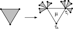
Fig. 1.–: First step in the construction of Husimi cactus with $K=3$ and connectivity $C=4$.

A Husimi cactus with connectivity $C$ is generated starting with a polygon of $K$ vertices with one Ising spin in each vertex (generation $0$). All spins in a polygon interact through a single coupling ${\cal J}_{\mu}$ and one of them is called the base spin. In figure 1 we show the first step in the construction of a Husimi cactus, in a generic step the base spins of the $n-1$ generation polygons, numbering $(C-1)(K-1)$, are attached to $K-1$ vertices of a generation $n$ polygon. This process is iterated until a maximum generation $n_{\mbox{max}}$ is reached, the graph is then completed by attaching $C$ uncorrelated branches of $n_{\mbox{max}}$ generations at their base spins. In that way each spin inside the graph is connected to exactly $C$ polygons. The local magnetisation at the centre $m_{j}$ can be obtained by fixing boundary (initial) conditions in the $0$-th generation and iterating recursion equations until generation $n_{\mbox{max}}$ is reached. Carrying out the calculation in the thermodynamic limit corresponds to having $n_{\mbox{max}}\sim\ln M$ generations and $M\rightarrow\infty$.

The Hamiltonian of the model has the form (2) where ${\cal L}(\mu)$ denotes the polygon $\mu$ of the lattice. Due to the tree-like structure, local quantities far from the boundary can be calculated recursively by specifying boundary conditions. The typical decoding performance can therefore be computed exactly without resorting to replica calculations [22].

We adopt the approach presented in [19] where recursion relations for the probability distribution $P_{\mu k}(\tau_{k})$ for the base spin of the polygon $\mu$ is connected to $(C-1)(K-1)$ distributions $P_{\nu j}(\tau_{j})$, with $\nu\in{\cal M}(j)\setminus\mu$ (all polygons linked to $j$ but $\mu$) of polygons in the previous generation:

$$P_{\mu k}(\tau_{k})=\frac{1}{{\cal N}}\mbox{ Tr}_{\{\tau_{j}\}}\exp\left[\beta\left({\cal J}_{\mu}\tau_{k}\prod_{j\in{\cal L}(\mu)\setminus k}\tau_{j}-1\right)+F\tau_{k}\right]\prod_{\nu\in{\cal M}(j)\setminus\mu}\prod_{j\in{\cal L}(\mu)\setminus k}P_{\nu j}(\tau_{j}),$$ (4)

where the trace is over the spins $\tau_{j}$ such that $j\in{\cal L}(\mu)\setminus k$.

The effective field $\widehat{x}_{\nu j}$ on a base spin $j$ due to neighbours in polygon $\nu$ can be written as :

$$\exp\left(-2\widehat{x}_{\nu j}\right)=\mbox{e}^{2F}\frac{P_{\nu j}(-)}{P_{\nu j}(+)},$$ (5)

Combining (4) and (5) one finds the recursion relation:

$$\exp\left(-2\widehat{x}_{\mu k}\right)=\frac{\mbox{ Tr}_{\{\tau_{j}\}}\exp\left[-\beta{\cal J}_{\mu}\prod_{j\in{\cal L}(\mu)\setminus k}\tau_{j}+\sum_{j\in{\cal L}(\mu)\setminus k}(F+\sum_{\nu\in{\cal M}(j)\setminus\mu}\widehat{x}_{\nu j})\tau_{j}\right]}{\mbox{ Tr}_{\{\tau_{j}\}}\exp\left[+\beta{\cal J}_{\mu}\prod_{j\in{\cal L}(\mu)\setminus k}\tau_{j}+\sum_{j\in{\cal L}(\mu)\setminus k}(F+\sum_{\nu\in{\cal M}(j)\setminus\mu}\widehat{x}_{\nu j})\tau_{j}\right]}.$$ (6)

By computing the traces and taking $\beta\rightarrow\infty$ one obtains:

$$\widehat{x}_{\mu k}=\mbox{atanh}\left[{\cal J}_{\mu}\prod_{j\in{\cal L}(\mu)\setminus k}\mbox{tanh}(F+\sum_{\nu\in{\cal M}(j)\setminus\mu}\widehat{x}_{\nu j})\right]$$ (7)

The effective local magnetisation due to interactions with the nearest neighbours in one branch is given by $\widehat{m}_{\mu j}=\mbox{tanh}(\widehat{x}_{\mu j})$. The effective local field on a base spin $j$ of a polygon $\mu$ due to $C-1$ branches in the previous generation and due to the external field is $x_{\mu j}=F+\sum_{\nu\in{\cal M}(j)\setminus\mu}\widehat{x}_{\nu j}$; the effective local magnetisation is, therefore, $m_{\mu j}=\mbox{tanh}(x_{\mu j})$. Equation (7) can then be rewritten in terms of $\widehat{m}_{\mu j}$ and $m_{\mu j}$ and the PP equations [3, 12, 20] can be recovered:

$$m_{\mu k}=\mbox{tanh}\left(F+\sum_{\nu\in{\cal M}(j)\setminus\mu}\mbox{atanh }(\widehat{m}_{\nu k})\right)\qquad\widehat{m}_{\mu k}={\cal J}_{\mu}\prod_{j\in{\cal L}(\mu)\setminus k}m_{\mu j}$$ (8)

Once the magnetisations on the boundary ($0$-th generation) are assigned, the local magnetisation $m_{j}$ in the central site is determined by iterating (8) and computing :

$$m_{j}=\mbox{tanh}\left(F+\sum_{\nu\in{\cal M}(j)}\mbox{atanh }(\widehat{m}_{\nu j})\right)$$ (9)

The free energy can be obtained by integration as (8) represents extrema of a free energy [15, 16, 23].

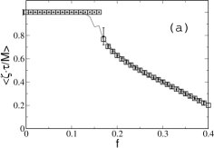
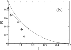
Fig. 2.–: (a) Mean normalised overlap between the actual noise vector ${\zeta}$ and decoded noise $\widehat{\mbox{\boldmath${\tau}$}}$ for $K=4$ and $C=3$ (therefore $R=1/4$). Theoretical values ($\Box$), experimental averages over $20$ runs for code word lengths $M=5000$ ($\bullet$) and $M=100$ (full line). (b) Transitions for $K=6$. Shannon’s bound (dashed line), information theory upper bound (full line) and thermodynamic transition obtained numerically ($\circ$). Theoretical ($\Diamond$) and experimental ($+$, $M=5000$ averaged over $20$ runs) PP decoding transitions are also shown. In both figures, symbols are chosen larger than the error bars.

By applying the gauge transformation ${\cal J}_{\mu}\mapsto 1$ and $\tau_{j}\mapsto\tau_{j}\zeta_{j}$, assigning the probability distributions $P_{0}(x)$ to boundary fields and averaging over random local fields $F\zeta$ one obtains from (7) the recursion relation in the space of probability distributions $P(x)$ [23]:

$$P_{n}(x) = \int\prod_{l=1}^{C-1}d\widehat{x}_{l}\;\widehat{P}_{n-1}(\widehat{x}_{l})\;\left\langle\delta\left[x-F\zeta-\sum_{l=1}^{C-1}\widehat{x}_{l}\right]\right\rangle_{\zeta}$$

$$\widehat{P}_{n-1}(\widehat{x}) = \int\prod_{j=1}^{K-1}dx_{j}\;P_{n-1}(x_{j})\;\delta\left[\widehat{x}-\mbox{atanh}\left(\prod_{j=1}^{K-1}\mbox{tanh}(x_{j})\right)\right],$$ (10)

where $P_{n}(x)$ is the distribution of effective fields at the $n$-th generation due to the previous generations and external fields, in the thermodynamic limit the distribution far from the boundary will be $P_{\infty}(x)$ (generation $n\rightarrow\infty$). The local field distribution at the central site is computed by replacing $C-1$ by $C$ in (10), taking into account $C$ polygons in the generation just before the central site, and inserting the distribution $P_{\infty}(x)$. Equations (10) are identical to those obtained by the replica symmetric theory as in [14, 15, 16].

By setting initial (boundary) conditions $P_{0}(x)$ and numerically iterating (10), for $C\geq 3$ one can find, up to some noise level $f_{s}$, a single stable fixed point at infinite fields, corresponding to a totally aligned state (successful decoding). At $f_{s}$ a bifurcation occurs and two other fixed points appear, stable and unstable, the former corresponding to a misaligned state (decoding failure). This situation is identical to that one observed in [14, 15, 16]. In terms of the local fields distribution $P_{n}(x)$, the aligned state corresponds to a runaway wave travelling to $x(n)\rightarrow\infty$ with $n$ being the time variable. The misaligned state corresponds to a stable wave located at $x(n)\sim{\cal O}(1)$. Representing the distributions (10) by the first cummulants only, one can obtain a rough approximation in terms of one dimensional maps showing a bifurcation at some noise level $\tilde{f}_{s}$, this approach will be further exploited elsewhere.

The practical PP decoding is performed by setting initial conditions as $m_{\mu j}=1-2f$ to correspond to the prior probabilities and iterating (8) until stationarity or a maximum number of iterations is attained [3]. The estimate for the noise vector is then produced by computing $\widehat{\tau}_{j}=\mbox{sign}(m_{j})$. At each decoding step the system can be described by histograms of the variables (8), this is equivalent to iterating (10) (a similar idea was presented in [3, 6]). Below $f_{s}$ the process always converges to the successful decoding state, above $f_{s}$ it converges to the successful decoding only if the initial conditions are fine tuned, in general the process converges to the failure state. In Fig.2a we show the theoretical mean overlap between actual noise ${\zeta}$ and the estimate $\widehat{\mbox{\boldmath${\tau}$}}$ as a function of the noise level $f$ as well as results obtained with PP decoding.

Information theory provides an upper bound for the maximum attainable code rate by equalising the maximal information contents of the syndrome vector ${z}$ and of the noise estimate $\widehat{\mbox{\boldmath${\tau}$}}$ [3, 16]. The thermodynamic phase transition obtained by finding the stable fixed points of (10) and their free energies interestingly coincides with this upper bound within the precision of the numerical calculation. Note that the performance predicted by thermodynamics is not practical as it requires ${\cal O}(2^{M})$ operations for an exhaustive search for the global minimum of the free energy. In Fig.2b we show the thermodynamic transition for $K=6$ and compare with the upper bound, Shannon’s bound and $f_{s}$ values.

Table I.–: Gallager versus MN codes

Gallager MN

dynamical variables M N+M

constraints M-N M

unbiased messages coding for all K K =1,2

Shannon’s bound K$$\rightarrow\infty$$ K 3 and unbiased messages

The geometrical structure of a Gallager code defined by the matrix ${A}$ can be represented by a bipartite graph (Tanner graph) [20] with bit and check nodes. Each column $j$ of ${A}$ represents a bit node and each row $\mu$ represents a check node, $A_{\mu j}=1$ means that there is an edge linking bit $j$ to check $\mu$. It is possible to show [24] that for a random ensemble of regular codes, the probability of completing a cycle after walking $l$ edges starting from an arbitrary node is upper bounded by ${\cal P}[l;K,C,M]\leq l^{2}K^{l}/M$. It implies that for very large $M$ only cycles of at least order $\ln M$ survive. In the thermodynamic limit $M\rightarrow\infty$ the probability ${\cal P}[l;K,C,M]\rightarrow 0$ for any finite $l$ and the bulk of the system is effectively tree-like. By mapping each check node to a polygon with $K$ bit nodes as vertices, one can map a Tanner graph into a Husimi lattice that is effectively a tree for any number of generations of order less than $\ln M$. It is experimentally observed that the number of iterations of (8) required for convergence does not scale with the system size, therefore, it is expected that the interior of a tree-like lattice approximates a Gallager code with increasing accuracy as the system size increases. Fig.2a shows that the approximation is fairly good even for sizes as small as $M=100$. Note that although the local magnetisations $m_{j}$ for a loopy graph are not generally expected to converge to the values computed in a tree, $\mbox{sgn}(m_{j})$ seems to do so. A thorough discussion on this respect for some specific graphical models can be found in [25].

In [3] MacKay and Neal introduced a variation on Gallager codes termed MN codes. The main difference between these codes is that for MN codes the syndrome vector contains also information on the original message in the form $\mbox{\boldmath${z}$}=\mbox{\boldmath${C_{s}}$}\mbox{\boldmath${\xi}$}+\mbox{\boldmath${C_{n}}$}\mbox{\boldmath${\zeta}$}$. The message itself is directly estimated and there is no need for recovering the noise vector. MacKay has formulated and proved a number of theorems simultaneously for both codes using the fact that if both message and noise are sampled from the same distribution, these codes can be formulated as the same estimation problem, to say, finding the most probable vector ${x}$ that satisfies $\mbox{\boldmath${z}$}=\mbox{\boldmath${A}$}\mbox{\boldmath${x}$}$, given the matrix ${A}$ and a prior distribution $P(\mbox{\boldmath${x}$})$. Using statistical physics, we previously analysed MN codes [14, 15, 16]. It is interesting to note that in spite of the similarity between the two codes, there are some important differences in their dependence on the parameters $K$ and $C$. In particular, Shannon’s bound is only attainable by Gallager codes if $K\rightarrow\infty$, in contrast to results obtained for MN codes. Decoding of unbiased messages is generally possible with Gallager codes, but successful convergence is only guaranteed (in the thermodynamic limit) for $K=1,2$ in the MN codes. We outlined those differences in table I.

To summarise, we solved exactly, without resorting to the replica method, a system representing a Gallager code on a Husimi cactus. The results obtained are in agreement with the replica symmetric calculation and with numerical experiments carried out in systems of moderate size. The framework can be easily extended to MN and similar codes. We believe that methods of statistical physics are complimentary to those used in the statistical inference community and can enhance our understanding of general graphical models beyond error-correcting codes.

***

We acknowledge support from EPSRC (GR/N00562), The Royal Society (RV,DS) and from the JSPS RFTF program (YK).

References

- [1] Shannon C., Bell Syst. Tech. J., 27 (1948) 379.
- [2] Viterbi A. J. and Omura J. K., Principles of Digital Communication and Coding, (McGraw-Hill Book Co., Singapore) 1979.
- [3] MacKay D. J. C. and Neal R. M., Electr. Lett., 32 (1996) 1645; MacKay D. J. C., IEEE Trans. Info. Theory, 45(1999) 399.
- [4] Gallager R. G., IRE Trans. Info. Theory, 8 (1962) 21.
- [5] Berrou G. et al., Proc. of the IEEE Int. Conf. on Comm., (Geneva) 1993 p. 1064.
- [6] Davey M. C., Record-braking error-correction using low-density parity-check codes, (Hamilton prize essay, University of Cambridge) 1998.
- [7] Kanter I.and Saad D., Phys. Rev. Lett., 83(1999) 2660; J. Phys A, 33 (2000) 1675.
- [8] Sourlas N., Nature, 339 (1989) 693; Europhys. Lett., 25(1994) 159.
- [9] Derrida B., Phys. Rev. B, 24 (1981) 2613.
- [10] Saakian D.B., Pis’ma Zh. Éksp. Teor. Fiz.[JETP Lett.], 67 (1998) 440.
- [11] Dorlas T.C. and Wedagedera J.R., Phys. Rev. Lett., 83 (1999) 4441.
- [12] Kabashima Y. and Saad D., Europhys. Lett., 44 (1998) 668; Europhys. Lett., 45 (1999) 97.
- [13] Vicente R., Saad D. and Kabashima Y., Phys. Rev. E, 60 (1999) 5352.
- [14] Kabashima Y., Murayama T. and Saad D., Phys. Rev. Lett., 84(2000) 1355.
- [15] Murayama T. et al. , Phys. Rev. E, 62 (2000) in press.
- [16] Vicente R., Saad D. and Kabashima Y., cond-mat/9908358 Preprint, 1999.
- [17] Montanari A., Sourlas N., cond-mat/9909018 Preprint, 1999; Montanari A., cond-mat/0003218 Preprint, 2000.
- [18] Dress C., Amic E. and Luck J.M., J. Phys. A, 28 (1995) 135.
- [19] Rieger H. and Kirkpatrick T.R., Phys. Rev. B, 45(1992) 9772.
- [20] Kschischang F. R. and Frey B. J., IEEE J. Select. Areas in Comm., 16(1998) 153.
- [21] Aji S.M. and McEliece R.J., IEEE Trans. Info. Theory, 46(2000) 325.
- [22] Gujrati P.D., Phys. Rev. Lett., 74(1995) 809.
- [23] Bowman D. R. and Levin K., Phys. Rev. B, 25 (1982) 3438.
- [24] Richardson T. and Urbanke R., Preprint, 1998.
- [25] Weiss Y., Neural Computation, 12 (2000) 1.