Band and filling controlled transitions in exactly solved electronic models

Abstract

We describe a general method to study the ground state phase diagram of electronic models on chains whose extended Hubbard hamiltonian is formed by a generalized permutator plus a band-controlling term. The method, based on the appropriate interpretation of Sutherland’s species, yields under described conditions a reduction of the effective Hilbert space. In particular, we derive the phase diagrams of two new models; the first one exhibits a band-controlled insulator-superconductor transition at half-filling for the unusually high value $U_{c}=6t$; the second one is characterized by a filling-controlled metal-insulator transition between two finite regions of the diagram.

1998 PACS number(s): 71.10.Pm; 71.27.+a; 05.30.-d

Metal-Insulator and Insulator-Superconductor Transitions in chain systems of interacting electrons have recently become a matter of great interest for the physics of new compounds and devices[1]. Although many experimental data are nowadays at disposal, an important open question of this issue is to determine the Hamiltonian that could fairly describe these kinds of transitions. The task is particularly difficult just owing to the low dimensionality, which causes usual mean-field and perturbative approaches to often fail in providing reliable predictions. Fortunately, 1-dimensionality allows to exploit exact analysis techniques which can provide –although only for some particular cases– rigorous informations on the structure of the ground state and on low-energy excitations. For this reason a probative test for theoretical models is the comparison between experimental results and theoretical predictions on the ground state phase diagram.
The ground state is usually given as a function of the filling $n$, i.e. the number of effective carriers, and of a ‘band-parameter’, which indicates the intrinsic unit of energy of the system (its actual definition depends on the theoretical approach envisaged, see below). One can thus distinguish between filling-controlled (FC) and band-controlled (BC) transitions, according to which kind of parameter (number of carriers or energy scale respectively) is tuned to let the transition occur. Both kinds of transitions are very important in practical applications: BC transitions are relevant for instance in Vanadium oxides, where one can modify the band-width through hydrostatic pressure on the sample; FC transitions are frequent in perovskite-like materials such as ${\mathrm{R}}_{1-x}{\mathrm{A}}_{x}{\mathrm{TiO}}_{3}$ (R=rare-earth ion, and A=alkaline-earth-ion), as well as in hole-doped compounds like ${\mathrm{La}}_{1-x}{\mathrm{Sr}}_{x}{\mathrm{CuO}}_{2.5}$. In order to describe these materials, at least as far as their low energy excitations are concerned, where single band picture are often reliable, the class of extended Hubbard models provides an interesting starting point. For these models, which involve strong electronic correlations, the band-parameter is usually [2] taken to be the on-site Coulomb repulsion ($U$), instead of $w=4t$ ($t$ = hopping amplitude), the latter being typical in mean-field approaches. A number of exact results have been obtained in terms of $n$ and $U$. For the ordinary Hubbard model, a FC metal-insulator-metal transition has been shown to occur at half filling ($n=1$) for any $U>0$ ($U$ being the on-site Coulomb repulsion); on the contrary, no BC transition takes place for $U>0$. More recently, some models ([3] and [4]) were solved in which a BC Insulator-Superconductor Transition occurs at half-filling at finite values of $U>0$, while the usual FC Metal-Insulator-Metal transition takes place for $n=1$ and $U>U_{c}$.
At the best of the authors’ knowledge, no detailed investigation has been devoted to either of the following issues: for the BC transitions it has not been pointed out yet what interaction terms are relevant to tune the critical value $U_{c}$ at which the transition occurs: this is quite important because $U_{c}$ can assume different values according to the chemical structure of the material. Secondly, for the FC transitions, all the above models provide an insulating state only at half filling; on the contrary, doped materials exhibit an insulating phase for a finite region of filling values. In this letter we examine the above subjects providing the exact ground state phase diagram of some 1-D electronic models. In particular, we obtain rigorous results which allow us to both discuss the dependence of $U_{c}$ of BC transitions on the Hamiltonian parameters, and to find a FC metal-insulator transition between two finite regions of the phase diagram.
We consider here the most general 1-band extended isotropic Hubbard model preserving the total spin and number $N$ of electrons, which reads

$${\cal H} =-\sum_{\langle{j},{k}\rangle,\sigma}[t-X(\hat{n}_{{j},-\sigma}+\hat{n}_{{k},-\sigma})+\tilde{X}\hat{n}_{{j},-\sigma}\hat{n}_{{k},-\sigma}]c_{{j},\sigma}^{\dagger}c_{{k},\sigma}+U\sum_{j}\hat{n}_{{j},\uparrow}\hat{n}_{{j},\downarrow}+{V\over 2}\sum_{\langle{j},{k}\rangle}\hat{n}_{j}\hat{n}_{k}$$ (1)

$$+ {W\over 2}\sum_{\langle{j},{k}\rangle,\sigma,\sigma^{\prime}}c_{{j},\sigma}^{\dagger}c_{{k},\sigma^{\prime}}^{\dagger}c_{{j},{\sigma}^{\prime}}c_{{k},\sigma}+Y\sum_{\langle{j},{k}\rangle}c_{{j},\uparrow}^{\dagger}c_{{j},\downarrow}^{\dagger}c_{{k},\downarrow}c_{{k},\uparrow}+P\sum_{\langle{j},{k}\rangle}\hat{n}_{{j},\uparrow}\hat{n}_{{j},\downarrow}\hat{n}_{k}+{Q\over 2}\sum_{\langle{j},{k}\rangle}\hat{n}_{{j},\uparrow}\hat{n}_{{j},\downarrow}\hat{n}_{{k},\uparrow}\hat{n}_{{k},\downarrow}\,,$$ (2)

In (1) $c_{{j},\sigma}^{\dagger},c_{{j},\sigma}\,$ are fermionic creation and annihilation operators on a 1-dimensional chain with $L$ sites, $\sigma\in\{\uparrow,\downarrow\}$, $\,\hat{n}_{{j},\sigma}=c_{{j},\sigma}^{\dagger}c_{{j},\sigma}$, $\hat{n}_{j}=\sum_{\sigma}\hat{n}_{{j},\sigma}$, and $\langle{j},\,{k}\rangle$ stands for neighboring sites. $t$ represents the hopping energy of the electrons (henceforth we set $t=1$), while the subsequent terms describe their Coulomb interaction energy in a narrow band approximation: $U$ parametrizes the on-site repulsion, $V$ the neighboring site charge interaction, $X$ the bond-charge interaction, $W$ the exchange term, and $Y$ the pair-hopping term. Moreover, additional many-body coupling terms have been included in agreement with [5]: $\tilde{X}$ correlates hopping with on-site occupation number, and $P$ and $Q$ describe three- and four-electron interactions. In the following we shall identify the 4 physical states $|\uparrow\rangle$, $|\downarrow\rangle$, $|0\rangle$ and $|\downarrow\uparrow\rangle$ at each lattice site with the canonical basis $e_{\alpha}$ of ${\mathbb{C}}^{4}$, and denote $n_{\uparrow}=N_{\uparrow}/L$; $n_{\downarrow}=N_{\downarrow}/L$; $n_{o}=N_{o}/L$; $n_{\uparrow\downarrow}=N_{\uparrow\downarrow}/L$ the densities of these 4 species of physical states.
In [6] it has been shown that, by fixing all the coupling constants of (1) to appropriate values, one can rewrite ${\cal H}$ as a generalized permutator (GP) between neighboring sites (minus some constant terms). Here we add to the latter a further arbitrary term $U\sum_{j}\hat{n}_{j\uparrow}\hat{n}_{j\downarrow}$, which is easily proved to commute with the GP. In matrix representation, the Hamiltonian (1) that we consider reads

$$H=-\sum_{\alpha\geq\beta}\,\Pi_{\alpha\beta}\,+\,UN_{\uparrow\downarrow}\,-\,const.terms$$ (3)

where $\Pi_{\alpha\beta}$ acts as a GP $\Pi$ (see below) whenever 2 neighboring sites of the chain are occupied by $e_{\alpha}$ and $e_{\beta}$, otherwise it gives zero. The constant terms are of the form ${\bar{U}}N_{\uparrow\downarrow}+\bar{\mu}N+\bar{c}\,{\mathbb{I}}$, where ${\bar{U}},{\bar{\mu}}$ and ${\bar{c}}$ are fixed values.
The purpose of this letter is to show how to investigate the ground state phase diagram of (3) as a function of the band parameter $U$ and the filling of the carriers $n$.

Let us first recall some basic properties of the GP’s. With respect to an ordinary permutator, a generalized permutator can either permute or leave unchanged the states of the 2 neighboring sites (including a possible additional sign); explicitly:

$$\Pi\,(e_{\alpha}\otimes e_{\beta})=\theta^{d}_{\alpha\beta}\,(e_{\alpha}\otimes e_{\beta})\,+\,\theta^{o}_{\alpha\beta}\,(e_{\beta}\otimes e_{\alpha})$$ (4)

where $\theta^{d}_{\alpha\beta}$ and $\theta^{o}_{\alpha\beta}$ are two discrete valued (0, -1 or 1) functions determining on $\Pi$ the positions and the signs of the diagonal and off-diagonal entries respectively. Also, $\theta^{d}$ and $\theta^{o}$ are ‘complementary’, i.e. $|\theta^{d}_{\alpha\beta}|=1-|\theta^{o}_{\alpha\beta}|$, so that $\Pi$ has only one non-vanishing entry for row or column. Moreover, $\theta^{o}_{\alpha\beta}=\theta^{o}_{\beta\alpha}$, hence $\Pi$ is a symmetric matrix. The set of couples of subscripts $(\alpha,\beta)$ for which $\theta^{d}_{\alpha\beta}\neq 0$ (resp.$\theta^{o}_{\alpha\beta}\neq 0$) is denoted by ${\cal A}^{d}$ (resp.${\cal A}^{o}$). It is easily seen that ${\cal A}^{d}$ is always of the form ${\cal A}^{d}=\cup_{i}\,{\cal S}_{i}\times{\cal S}_{i}$, the ${\cal S}_{i}$’s being disjoint subsets of the set ${\cal S}=\{1,2,3,4\}$. By varying the functions $\theta^{d}$ and $\theta^{o}$ one obtains different kinds of GP’s.

In order to determine the ground state phase diagram of (3), the difficult task is to calculate the contribution to the energy of the first term. To solve this issue, one can reconduct it to a problem defined in a smaller Hilbert space. Indeed it can be seen that:

1) Under the conditions precised below, a generalized permutator between physical states is equivalent to an ordinary permutator between the so called Sutherland’s species (SS). The latter do not need to be identified with the physical species (PS) of the states. Indeed, the number of PS is determined by the nature of the problem (in our cases they are always the four $e_{\alpha}$), while the number of SS is determined by the structure of the GP entering the Hamiltonian. In particular, it may happen that different PS constitute a single SS, so that the number of the latter is $\leq 4$, leading to a reduction of the dimensionality of the effective Hilbert space. Through a suitable identification of the Sutherland’s species, the first term of (3) can be rewritten in the form:

$$H_{0}=-\sum_{A}p_{A}N_{AA}-\sum_{A>B}\sigma_{AB}\Phi_{AB}\quad,$$ (5)

where $p_{A}=\pm 1$ determines the nature of the $A$-th species, even (${\cal E}$)/odd (${\cal O}$) for $+1/-1$; $N_{AA}$ is the number of neighboring sites occupied by the same species $A$, and $\Phi_{AB}$ permutes objects of species $A$ and $B$ that occupy two neighboring sites, otherwise it gives zero. The $\sigma_{AB}$ are signs. For a given GP, the SS are to be identified through the subsets ${\cal S}_{i}$’s of ${\cal A}^{d}$. In practice, the reduction to Sutherland’s species is possible if: $a)$ $\theta^{d}_{\alpha\beta}=p_{i}\,\,\forall\alpha,\beta\in{\cal S}_{i}$ and $b)$ $\theta^{o}_{\alpha\beta}=\sigma_{ij}\,,\,\forall\alpha\in{\cal S}_{i}\,,\,\forall\beta\in{\cal S}_{j}$, where $i\neq j$.

2) In the case where (5) has $\sigma_{AB}$=+1 $\forall\,A,B\in{\cal E}$, and $\sigma_{AB}$ independent of $B$ for $B\in{\cal O}$ and $A\in{\cal E}$ (Sutherland’s Hamiltonian), it is possible to reduce the number of even species down to only one. Indeed in this case the ground state energy of hamiltonian (5) for a system with $x$ even species and $y$ odd species is equal to that of the same hamiltonian acting on a system with the same number of odd species but just one even species collecting all the previous ones (as implied by a simple extension of Sutherland’s theorem, see [7]).

Remark: For a given GP, the fulfillment of the conditions given at points 1) and 2) depends also on the normalization chosen to define the basis vectors. It is worth emphasizing that some GP, though apparently violating the above requirements, can be brought to fulfill them through a mere redefinition of the phase of a given physical species $\bar{\alpha}$, i.e. $|e_{\bar{\alpha}}\rangle_{j}\rightarrow(-1)^{j}|e_{\bar{\alpha}}\rangle_{j}$. We shall make use of this remark in the following.

To illustrate how the above observations can be exploited, we start with a known case, the AAS model [4], which differs from the ordinary Hubbard model only for a correlated-hopping term ($X=1;\tilde{X}=V=W=Y=P=Q=0$). This model is of the form (3), with ${\bar{U}}=-4$, $\bar{\mu}=2$, and $\bar{c}=-1$. Its GP reduces to (5) by identifying the following two Sutherland’s species: $A=\{|\uparrow\rangle,|\downarrow\rangle\}$ (odd) and $B=\{|0\rangle,|\downarrow\uparrow\rangle\}$ (even). In this formalism the model is nothing but a free spinless fermion model, and its energy per site is given by

$$\epsilon=2n_{A}-1-{2\over\pi}\sin(\pi n_{A})+(U-{\bar{U}})n_{\uparrow\downarrow}-\bar{\mu}n-\bar{c}\,,$$ (6)

where $n_{A}=n_{\uparrow}+n_{\downarrow}$. The phase diagram as a function of the filling $n=N/L$ and $U$ can be easily derived by exploiting the identity $n_{\uparrow\downarrow}=(n-n_{A})/2$ and minimizing $\epsilon$ with respect to $n_{A}$ ($n_{A}\in[0,n]$ for $0\leq n\leq 1$ and $n_{A}\in[0,2-n]$ for $1\leq n\leq 2$) and coincides with that derived in [4]. We also notice that the model with $X=1;\tilde{X}=2;V=W=Y=P=Q=0$ has the same energy as AAS. In fact, using the above Remark and redefining the basis vector $|\downarrow\uparrow\rangle_{j}\rightarrow(-1)^{j}|\downarrow\uparrow\rangle_{j}$, it can be cast in the form (3) with the same GP as AAS.

The method just outlined allows the solution of a wide class of models whose Hamiltonian has the form (3)[6]. In particular, as the AAS model displays both a BC and a FC transitions, here we apply it to the study of similar, but new, models in which further terms are included, yielding a change in the value of the parameters characterizing the transition. We consider the model with coupling constants $X=1;\tilde{X}=(1-\sigma);Y=-\sigma;P=-1;Q=2$ where $\sigma=\pm 1$. The resulting Hamiltonian has the form (3) with ${\bar{U}}=-2$, $\bar{\mu}=2$, $\bar{c}=-1$ in both cases $\sigma=\pm 1$. $\Pi$ has diagonal entries characterized by the subsets ${\cal S}_{1}=\{1,2\}$ , ${\cal S}_{2}=\{3\}$ , ${\cal S}_{3}=\{4\}$, and off-diagonal entries $\theta^{o}_{\alpha\beta}=+1$ $\forall\alpha\in{\cal S}_{1}\,,\,\beta\in{\cal S}_{2}$ and $\theta^{o}_{\alpha\beta}=\sigma$ $\forall\alpha\in{\cal S}_{1}$ or ${\cal S}_{2}\,,\,\beta\in{\cal S}_{3}$. Both the conditions $a)$ and $b)$ to identify Sutherland’s species are thus fulfilled, and the species read: $A=\{|\uparrow\rangle,|\downarrow\rangle\}$ (which is ‘odd’ because $\theta^{d}_{\alpha\beta}=-1$ if $\alpha,\beta\in{\cal S}_{1}$) ; $B=|0\rangle$ (‘even’ because $\theta^{d}_{33}=+1$) and $C=|\downarrow\uparrow\rangle$ (‘even’ because $\theta^{d}_{44}=+1$). For the case $\sigma=+1$ one can straightforwardly apply Sutherland’s theorem (see point 2)) to reduce the number of even species to 1, ending up with a free spinless fermion problem, where occupied sites are represented by $A$ and empty sites by $B$ and $C$. The ground state energy $\epsilon$ per site has the same form as (6), in which again $n_{\uparrow\downarrow}=(n-n_{A})/2$, and it has to be minimized with respect to $n_{A}$. For the case $\sigma=-1$, before using Sutherland’s theorem, one has to apply again the Remark, changing $|\downarrow\uparrow\rangle_{j}\rightarrow(-1)^{j}|\downarrow\uparrow\rangle_{j}$. The expression of $\epsilon$ is identical.
The phase diagram is given in fig.1; the lower region I is characterized by $n_{A}=0$, so that only doubly occupied or empty sites are present in the ground state; in this region the ground state $|\Psi_{0}\rangle$ is made of the so-called (pure) eta-pairs, i.e. $|\Psi_{0}\rangle=(\eta^{\dagger}_{\varphi})^{N/2}|0\rangle$, where $\eta^{\dagger}_{\varphi}=\sum_{j}e^{i\varphi j}c^{\dagger}_{j\uparrow}c^{\dagger}_{j\downarrow}=\sum_{k}c^{\dagger}_{k\uparrow}c^{\dagger}_{\varphi-k\downarrow}$ with pair momentum $\varphi=0,\pi$. In the case $\sigma=+1$ we have 0-pairs, whereas if $\sigma=-1$ the pairs have $\pi$-momentum. The latter case is particularly important because the $\pi$-pairs (and not $0$-pairs) are expected to survive as the constraint $X=1$ is relaxed (see [8]). In region II, delimited by $U_{\mbox{II-III}}=2-4\cos(\pi n)$, we have the simultaneous presence of empty ($\circ$), singly occupied ($\circ$ $\mathbf{\shortmid}\hskip 4.19998pt$) and doubly occupied ($\bullet$) sites; this is called mixed region and the ground state is $|\Psi_{0}\rangle=(\eta^{\dagger}_{\varphi})^{N/2}|U=\infty\rangle$, where $|U=\infty\rangle$ are the eigenstates of the $U=\infty$ Hubbard model[5]. In both region I and II the ground state is superconducting, because the 2-particle reduced density matrix exhibits long range correlation[4], i.e. $g(i,j)=\langle\Psi_{0}|c^{\dagger}_{i\uparrow}c^{\dagger}_{i\downarrow}c_{j\downarrow}c_{j\uparrow}|\Psi_{0}\rangle\,\nrightarrow 0$ for $|i-j|\rightarrow+\infty$. Finally, the region III-a ($0\leq n\leq 1$) is made of singly occupied and empty sites; in this region the ground-state of the $U=\infty$ Hubbard model is eigenstate of the Hamiltonian and is metallic. The region III-b ($1\leq n\leq 2$) is the particle-hole transformed of III-a, and the metallic carriers are holes. One can show that at half-filling the system is an insulator with gap $\Delta=U-6$.
With respect to the AAS model we observe that the pair-hopping term has two main effects: first it removes the degeneracy in $\varphi$ in this region (only $\varphi=0$ or $\pi$ survive, according to the sign $\sigma$ of $Y$); secondly it raises the borderline of such region upwards: in fact it can be generally shown [9] that a pair hopping term acts as an effective attraction ($\propto\,-|Y|$) renormalizing the Coulomb repulsion $U$. The superconducting region II of our model is enhanced also with respect to that of the EKS model. Indeed, although the pair-hopping term is also present in the EKS model (the borderlines of region I coincide), its effect is strongly reduced near half-filling due to the Coulomb attraction term between neighboring sites ($V=-1$), which is known to compete with the formation of on-site pairs.
As a consequence, the BC insulator-superconductor transition occurring at half-filling corresponds to the maximum critical value $U_{c}^{max}=6$, higher than for all other exactly solved models. This is important because higher values of $U_{c}$ reduce the probability that thermal fluctuations may destroy the superconducting phase.

Because of the particle-hole symmetry of the models we have considered so far, the insulating phase can exist just at half filling. In order to investigate FC transitions between finite metal-insulator regions of the phase diagram, we now discuss a simple model not particle-hole invariant, describing a competition between the $U=\infty$ Hubbard model (excluding doubly-occupancy), and the pair-hopping (favouring the formation of pairs), modulated by the band parameter $U$ (explicitly $X=\tilde{X}=1$; $Y=\sigma$; $V=W=P=Q=0$). It is easy to realize that (up to the application of the Remark) this model can be set in the form (3) (${\bar{U}}=-2$, $\bar{\mu}=2$, and $\bar{c}=-1$). The GP is now equivalent to an ordinary permutation between the two Sutherland’s species: $A=\{|\uparrow\rangle,|\downarrow\rangle,|\downarrow\uparrow\rangle\}$ (which is ‘odd’ because $\theta^{d}_{\alpha\beta}=-1$ if $\alpha,\beta\in{\cal S}_{1}=\{1,2,4\}$); $B=|0\rangle$ (‘even’ because $\theta^{d}_{33}=+1$). The ground state energy per site is still given by eq. (6), where now $n_{\uparrow\downarrow}=n-n_{A}$, . The phase diagram –obtained by minimizing $\epsilon$ at fixed $n$ with respect to $n_{A}$ in the range $n/2\leq n_{A}\leq\min(n,1)$– is presented in fig. 2, and exhibits again four regions. However, due to the absence of particle-hole invariance, the shape is not symmetric around half-filling.
In region I (just doubly occupied and empty sites) only the $Y$ and $U$ terms act: the model behaves like a spin isotropic XX model ($\tilde{S}^{+}_{i}=c^{\dagger}_{i\uparrow}c^{\dagger}_{i\downarrow}$, $\tilde{S}^{-}_{i}=c_{i\downarrow}c_{i\uparrow}$) with the $U$ term acting as a magnetic field; it is well known that at $U=0$ the correlation function has a power law decay $g(i,j)\propto|i-j|^{-1/2}$, whereas $g$ is not known for non-vanishing magnetic field. However, as far as $U\leq 2$, long-range order arises for any non-zero value of anisotropy. The borderline of this region is given by $U_{\mbox{I-II}}=-2\cos(\pi n/2)$. Notice that this region raises up to positive values of $U$ for $1\leq n\leq 2$. The mixed region II is entered as the double occupancy begins to decrease from its maximum value, yielding the increase of the local magnetic moment $M_{0}=3/4\,L^{-1}\sum_{j}\langle\Psi_{0}|(\hat{n}_{j,\uparrow}-\hat{n}_{j,\downarrow})^{2}|\Psi_{0}\rangle=$ $3/4\,(2\pi^{-1}\arccos(-U/2)-n)$. The value of $n_{\uparrow\downarrow}$ reaches its minimum for $U_{\mbox{II-IIIa}}=-2\cos(\pi n)$ when $n\leq 1$, and for $U_{\mbox{II-IIIb}}=2$ when $n\geq 1$. Correspondingly, regions III-a and III-b are entered. The former is metallic, the ground-state is that of the $U=\infty$ Hubbard model, and the system behaves like a Tomonaga-Luttinger liquid. The most interesting feature is that region III-b is a finite insulating region. More precisely, at exactly half filling the gap is $\Delta=U-2$, while for $1<n\leq 2$ no empty site is present, and the model behaves like the Hubbard model in the atomic limit. Hence here the FC transition takes place between two finite regions, in analogy with experimental observations on chain hole-doped compounds. Interestingly, for the the special value $U=2$, our model and the $U$-supersymmetric model coincide. As a consequence, our ground state energy in this case is equal to that obtained in [10].

In this letter we have presented exact ground state phase diagrams of two electron models, and studied their BC and FC transitions. Our analysis supports the relevance of the pair-hopping term in raising the critical value of $U$ for BC superconducting-insulator transitions, as well as the importance of particle-hole not invariant terms in the apperance of a finite insulating region. The method we used can be implemented on all those models described by Hamiltonian (3) in which the GP verifies conditions a) and b). We stress that such GPs all correspond to integrable models [6], i.e. they are solutions of the Yang-Baxter Equation (consistency equation for factorizability). The Hamiltonians exhibit therefore a set of conserved quantities mutually commuting.

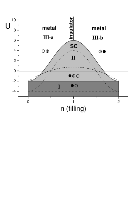
FIG. 1.: Ground state phase diagram of the model $X=1;\tilde{X}=(1-\sigma);Y=-\sigma;P=-1;Q=2$. The model exhibits a BC transition insulator-superconductor transition at $n=1$, for $U_{c}=6$. The dashed line is the EKS model, and the dotted line corresponds to the AAS model.

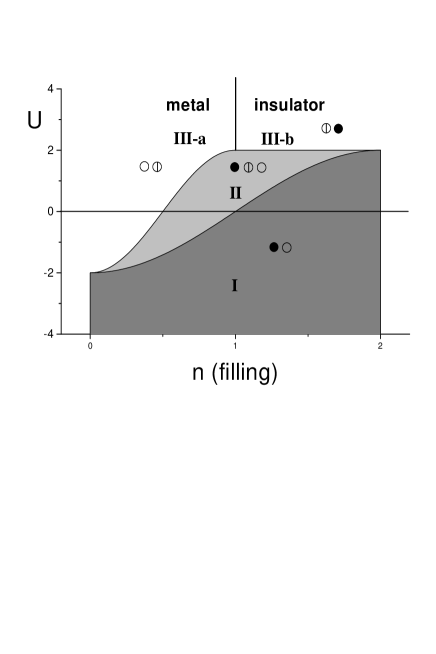
FIG. 2.: Ground state phase diagram of the model $X=\tilde{X}=1$ ; $Y=\sigma$; $V=W=P=Q=0$. A FC metal-insulator transition takes place for $U\geq 2$ between two finite regions, III-a and III-b.

REFERENCES

- [1] M.Dumm et al., Phys. Rev. B 61, 511 (2000); R. Farchioni, P. Vignolo, and G. Grosso, Phys. Rev. B 60, 15705 (1999); E. Chow, P. Delsing and D.B. Haviland, Phys. Rev. Lett. 81, 204 (1998)
- [2] M. Imada, A. Fujimori, Y. Tokura, Rev. Mod. Phys. 70, 1039 (1998)
- [3] F.H. Essler, V. Korepin, and K. Schoutens, Phys. Rev. Lett. 68, 2960 (1992); Phys. Rev. Lett. 70, 73 (1993)
- [4] L.Arrachea, and A.Aligia, Phys. Rev. Lett. 73, 2240 (1994); A.Schadschneider, Phys. Rev. B 51, 10386 (1995)
- [5] J. de Boer, V. Korepin, A. Schadschneider, Phys. Rev. Lett. 74, 789 (1995); C. Castellani, C. Di Castro, M. Grilli, Phys. Rev. Lett. 72, 3626 (1994)
- [6] F. Dolcini, and A. Montorsi, Int. J. Mod. Phys. B (to be published)
- [7] B. Sutherland, Phys. Rev. B 12, 3795 (1975)
- [8] A. Montorsi, and D.K. Campbell, Phys. Rev. B 53, 5153 (1996)
- [9] S. Robaszkiewicz, B.Bulka, Phys. Rev. B 59, 6430 (1999)
- [10] G.Bedürftig, H. Frahm, J.Phys. A; 28 4453 (1995)