On nonlinear susceptibility in supercooled liquids

Abstract

In this paper, we discuss theoretically the behavior of the four point nonlinear susceptibility and its associated correlation length for supercooled liquids close to the Mode Coupling instability temperature $T_{c}$. We work in the theoretical framework of the glass transition as described by mean field theory of disordered systems, and the hypernetted chain approximation. Our results give an interpretation framework for recent numerical findings on heterogeneities in supercooled liquid dynamics.

1 Introduction

Recently, a lot of attention has been devoted to understanding the nature of dynamical heterogeneities in supercooled liquids [1, 2, 3, 4, 5, 6, 7]. Many numerical experiments have found long lived dynamical structures which are characterized by a typical length and a typical relaxation time which depend on the values of the external parameters (temperature and density). A way to quantify this dynamical heterogeneities is in terms of the 4-point density function, and its associated non-linear susceptibility, which show power law behavior as one approaches the Mode Coupling temperature $T_{c}$ from above. In this paper we review the details of the theoretical calculations of this function put forward in [8, 9, 10] and discuss some new results.

At the glass transition one observes freezing of density fluctuations. The function

$$g_{2}(x)=\langle(\rho(x+y)-\overline{\rho})(\rho(y)-\overline{\rho})\rangle$$ (1)

is often regarded as the Edwards-Anderson order parameter signaling the onset of glassiness. It is therefore quite natural to try to interpret the dynamical heterogehinities and the correlation length in terms of fluctuations of the order parameter, and study the 4-point function

$$g_{4}(x)=\langle[(\rho(x+y)-\overline{\rho})(\rho(y)-\overline{\rho})]^{2}\rangle-\langle(\rho(x+y)-\overline{\rho})(\rho(y)-\overline{\rho})\rangle^{2},$$ (2)

and its related non-linear susceptibility $\chi_{4}=\int dxg_{4}(x)$. To our knowledge the first proposal to study the 4-point function to identify a growing correlation length in structural glasses was in [11] in the context of a numerical study of a Lennard-Jones liquid. There no sign of growing correlation was found, probably because of the insufficient thermalization. However, more accurate measurements [4, 5, 9, 12] show that there is a dynamical correlation length which grows as $T_{c}$ is approached.

Here we would like to investigate theoretically the behavior this function in the context of the picture of the glass transition that comes out from the study of disordered mean-field models [13], and from some approximation scheme of molecular liquids [14].

In mean field disordered systems one finds that decreasing the temperature from the liquid phase, two different transitions appear: a dynamical transition at a temperature $T_{c}$, and a static (Kauzmann-like) transition at a lower temperature $T_{K}$. At the dynamical transition $T_{c}$, identified with the Mode Coupling Theory [15] transition temperature, equilibrium density fluctuations freeze and ergodicity breaks down. Below that temperature, the Boltzmann distribution is decomposed in an exponentially large number of ergodic components $\rme^{N\Sigma(T)}$. $\Sigma(T)$, the logarithm of the number of these components is the configurational entropy, which decreases for decreasing temperatures, and the “static” transition signals the point where $\Sigma(T_{K})=0$. Dynamically, a non zero Edwards-Anderson order parameter signals freezing.

As it has been many times remarked, this theory misses the existence of local activated processes which restore ergodicity below $T_{c}$. These can be included phenomenologically to complete the picture. We will suppose that the ergodic components which the ideal theory predicts below $T_{c}$ become in real systems metastable states (or quasistates), capable to confine the system for some large, but finite times on given portions of the configuration space. The inclusion of activated processes, although done by hand, has far reaching consequences.

The foundation of the notion of quasistates is based on the time scale separation (as it can be seen in the shape of the structure function), which allows to consider “fast” degrees of freedom quasi-equilibrated, before the “slow” degrees of freedom can move. So, this notion applies below as well as above $T_{c}$, where the two step relaxation is predicted even by the ideal theory. This point has been recently stressed in [16] in a different context. Both above and below $T_{c}$ we can talk of quasistates in which the system equilibrates almost completely before relaxing further. The typical life time of the quasistate will be of the order of the alpha relaxation time $\tau_{\alpha}$.

Our basic observation is that within the described theoretical framework, the quasistates correspond to highly correlated regions of the configuration space, typical configurations belonging to the same quasistate would appear to be highly correlated. On the other hand, configurations belonging to distant quasistates as the ones which correspond to large time separation $t>>\tau_{\alpha}$, show typically low correlations.

We argue then, that the dynamical correlation length and susceptibility observed in the simulations referred to above, can be estimated by the corresponding quantities within a quasistate. On the other hand, the long time limit of the same quantities, i.e. the value reached for times much larger then the lifetime of the quasistates, correspond to maximally distant quasistates. This predicts maximal fluctuations and heterogeneity on a time scale of the order of $\tau_{\alpha}$.

2 How to compute quasistate averages: “recipes for metastable states”

In this section, we address the question on how to compute correlation functions within singles quasistates, reviewing some “recipes” that were put forward in [17, 18]. Let us consider the case of mean-field spin glass models below $T_{c}$, where there is true ergodicity breaking and the quasistates are true ergodic components. Suppose to be above $T_{K}$ so that the configurational entropy $\Sigma(T)>0$. Given any local observable $A(x)$, its Boltzmann average can be decomposed as

$$\langle A(x)\rangle_{Boltzmann}=\sum_{\alpha}w_{\alpha}\langle A(x)\rangle_{\alpha},$$ (3)

where the index $\alpha$ runs over all the $e^{N\Sigma}$ states, the weights of the different states $w_{\alpha}$ would all be of the same order $w_{\alpha}\approx\exp(-N\Sigma(T))$. In the following we will be interested to compute space averages (correlation functions) among local observables, $\int dx\langle A(x)\rangle\langle B(x+y)\rangle$. If by $\langle\cdot\rangle$ we mean Boltzmann average, we can expand each of the two averages according to (3) and find that

$$\int dx\langle A(x)\rangle\langle B(x+y)\rangle=\int dx\sum_{\alpha,\beta}w_{\alpha}w_{\beta}\langle A(x)\rangle_{\alpha}\langle B(x+y)\rangle_{\beta},$$ (4)

which, due to the fact that the number of ergodic components is exponentially large, is dominated by the terms in the double sum with $\alpha\neq\beta$.

Our major interest will be to compute instead averages of the kind $\int dx\sum_{\alpha}w_{\alpha}\langle A(x)\rangle_{\alpha}\langle B(x+y)\rangle_{\alpha}$ i.e. correlation function in the same ergodic component. To this purpose we can use a conditional Boltzmann prescription [17, 18], where one fixes a reference configuration $Y=\{y_{1},...,y_{N}\}$, and only the configurations $X=\{x_{1},...,x_{N}\}$ similar enough to the reference configuration are given a non vanishing weight.

Let us consider as a notion of similarity among two configurations $X$ and $Y$ the function, that we call overlap,

$$q(X,Y)=\int dxdy(\rho_{X}(x)-\overline{\rho})(\rho_{Y}(y)-\overline{\rho})w(|x-y|)$$ (5)

where:

• $\rho_{Z}(z)$ ($Z=X,Y$) is the microscopic density corresponding to the configuration $Z$: $\rho_{Z}(z)=\sum_{i}\delta(z_{i}-z)$

• the function $w(r)$ is a short range sigmoid (or step) function such that if $r_{0}$ denotes the typical radius of the particles, $w(r)$ is close to 1 for $r\leq ar_{0}$ and close to zero otherwise. The value of $a=0.3$ gives a notion of overlap not too sensitive to small atomic displacements.

Notice that with this definition $q(X,Y)$ is maximal if $X=Y$, while it is equal to zero if $X$ and $Y$ are uncorrelated. Notice also that one can write $q(X,Y)=\sum_{i,j}w(|x_{i}-y_{j}|)$, a form which is manifestly invariant under permutations of the particles.

Suppose now to fix a reference configuration $Y$, chosen with Boltzmann probability at temperature $T$, and consider the conditional probability

$$P_{q}(X|Y)=\frac{e^{-\beta H(X)}\delta(q(X,Y)-q)}{Z_{q}(Y)}$$ (6)

where the constrained partition function is

$$Z_{q}(Y)={\int dXe^{-\beta H(X)}\delta(q(X,Y)-q)}.$$ (7)

As $Y$ by hypothesis is an equilibrium configuration, it will belong to some quasistate $\alpha$, so, if we choose $q$ as the typical overlap among configurations in this quasistate (with probability one almost all configurations have the same overlap), i.e. the Edwards-Anderson parameter of the state $q_{EA}$, we will be able to compute the quasistate averages: given two observables $A(X)$ and $B(X)$ we can write:

$$\sum_{\alpha}w_{\alpha}\langle A\rangle_{\alpha}\langle B\rangle_{\alpha}=\int dY\frac{e^{\-\beta H(Y)}}{Z}A(Y)\int dX\frac{e^{-\beta H(X)}\delta(q(X,Y)-q)}{Z_{q}(Y)}B(X)$$ (8)

Notice that, if on the other hand in (6) we would choose $q$ as the typical overlap among different quasistates, the constraint would be completely irrelevant and we could get the Boltzmann average (4).

Notice that the overlap we consider, is a masked integral of the density-density correlation function among the two configurations $X$ and $Y$. We are interested to study the fluctuation of this quantity, which is the following integral of the 4-point function:

$$\chi_{4}= \beta(\overline{\langle q\rangle^{2}}-\overline{\langle q\rangle}^{2})$$

$$= \int\;dx\;dy\;dz\;drw(x-y)w(z-r)$$ (9)

$$\left(\overline{\langle(\rho_{X}(x)-\overline{\rho})(\rho_{Y}(y)-\overline{\rho})\rangle\langle(\rho_{Y}(z)-\overline{\rho})(\rho_{Z}(r)-\overline{\rho})\rangle}\right.$$

$$\left.-\overline{\langle(\rho_{X}(x)-\overline{\rho})(\rho_{Y}(y)-\overline{\rho})\rangle}\times\overline{\langle(\rho_{X}(z)-\overline{\rho})(\rho_{Y}(r)-\overline{\rho})\rangle}\right)$$

where we have denoted with the angular brackets the conditional average with the distribution (6), and with the bar the average over the canonical distribution of the reference configuration $Y$.

Within this formalism, the generating functional of the correlation functions is the constrained free-energy

$$V(q)=-\beta/N\int dY\frac{e^{\-\beta H(Y)}}{Z}\log(Z_{q}(Y)).$$ (10)

This function has been computed in various models having a glass transition, including mean field disordered models and simple liquids in the HNC approximation, all giving consistent results [17, 18]. The shape of $V$ as a function of $q$ allows to distinguish among liquid and glass phase. We show the potential in figure 1 for hard spheres in the HNC approximation.

In the liquid phase at high temperature, the potential is convex with a unique minimum for $q=0$ which corresponds to the typical overlap among random liquid configurations. Lowering the temperature, the potential looses the convexity, until, when $T_{c}$ is reached, it develops a secondary minimum, at a high value of $q$. The height of the secondary minimum with respect to the first one is related to the configurational entropy by: $V_{sec}-V_{pri}=T\Sigma(T)$, which vanishes at $T_{K}$.

Figure 1: The potential for HNC hard spheres at several densities. We show the high and low $q$ regions of the potential. The lines joining them are just guides for the eyes.Lower curves correspond to higher densities. At low density the potential is convex. The appearance of a secondary minimum signals the breaking of ergodicity, with exponentially many states.

A remarkable fact that has been often discussed [17], is that while the properties of the low $q$ minimum reflect the properties of the full Boltzmann average, the properties of the high $q$ minimum reflect the properties of averages in a single ergodic component.

In the shape of the potential the MC transition appears as a spinodal point and as such it has a divergent susceptibility. In fact, general relations in the effective potential theory, imply that the susceptibility is given just by the inverse curvature of the potential in the minimum, i.e. $\chi_{4}=1/V^{\prime\prime}(q)|_{secondary\;\;minimum}$. This quantity, diverges for $T\to T_{c}$, which, in turn, implies the divergence of the spatial range of the correlations. Generically, in all the model studied, the slope of the flex vanishes linearly for $T\to T_{c}$, implying $\chi_{4}(T)\simeq|T-T_{c}|^{-\gamma}$ with a mean field exponent $\gamma=1/2$. We notice that $\chi_{4}$ computed in the primary minimum represents the Boltzmann average of the order parameter fluctuations and is completely regular at $T_{c}$.

In figure 2 we see the susceptibility computed with this procedure (circles), which shows a divergence at $T_{c}$.

Figure 2: The susceptibility of the metastable states for the $p$-spin model with $p=3$. Here $T_{c}=0.612$. The low temperature data come from the potential theory. The high temperature data from the dynamical equations.

3 A dynamical approach

The idea of considering a system coupled with a reference configuration can also be used in dynamics to compute the time dependent susceptibility. In this context it is convenient to couple with the initial configuration $X_{0}$. Consider a system at equilibrium at time zero with respect to the Hamiltonian $H(X)$ which evolves for positive times with the modified Hamiltonian

$$H_{tot}(X)=H(X)-\epsilon q(X,X_{0}).$$ (11)

For small $\epsilon$, linear response theory at equilibrium implies that

$$\chi_{4}(t)=\beta\left(\langle q(X_{t},X_{0})^{2}\rangle-\langle q(X_{t},X_{0})q(X_{0},X_{0})\rangle\right)=\frac{\partial\langle q(X_{t},X_{0})\rangle}{\partial\epsilon}$$ (12)

The problem of studying the evolution of a system with Hamiltonian (11) can in principle be issued within any dynamical approximation scheme (e.g. MCT).

However for the time being we have only addressed the problem in the context of the p-spin model, which, for all the present purposes should capture the essential features of the function $\chi_{4}(t)$. Clearly, lacking completely in the model any spatial structure, in order to infer from the behavior of $\chi_{4}$ something about a correlation length we need to resort to eq. 9.

The p-spin model [19] describes $N$ interacting variables $S_{1},...,S_{N}$ (spins) on the sphere $\sum_{i}S_{i}^{2}=N$, with Hamiltonian $H=\sum_{i_{1}<...<i_{p}}J_{i_{1}...i_{p}}S_{i_{1}}...S_{i_{p}}$ where the couplings are random independent Gaussian variables with zero mean and variance $J^{2}=p!/(2N^{p-1})$. The appropriate notion of overlap for this system is $q(S,S^{\prime})=1/N\sum_{i}S_{i}S^{\prime}_{i}$. For this model it is customary to consider Langevin dynamics, which in our case will be performed with Hamiltonian $H_{tot}(S)=H(S)-\epsilon q(S,S_{0})$, where $S_{0}=S(t=0)$ is an equilibrium initial condition.

$$\frac{dS_{i}(t)}{dt}=-\frac{\partial H(S(t))}{\partial S_{i}}+\epsilon S_{i}(0)+\eta_{i}(t)$$ (13)

where $\eta_{i}(t)$ is a white noise with amplitude $2T$ and $\mu(t)$ is a Lagrange multiplier which ensures the spherical constraint at all times.

Using standard manipulations based on the Martin-Siggia-Rose functional integral, one can write a self consistent equation for a single spin which, using the notation $f(q)=1/2q^{p}$, reads:

$$\frac{dS(t)}{dt}= -\mu(t)S(t)+\int_{0}^{t}ds\;f^{\prime\prime}(C(t,s))R(t,s)S(s)$$ (14)

$$+\beta f^{\prime}(C(t,0))S(0)+\epsilon S(0)+\xi_{i}(t)$$

where $\xi(t)$ is a colored Gaussian noise with variance

$$\langle\xi(t)\xi(s)\rangle=f^{\prime}(C(t,s))+2T\delta(t-s)$$ (15)

where $C$ and $R$ are the correlation and response functions of the system, to be determined self-consistently by $C(t,s)=<S(t)S(s)>$, $R(t,s)=\langle\frac{\delta S(t)}{\delta\xi(s)}\rangle$. The detailed derivation of (14) is rather standard (see e.g. [20]) and we do not reproduce it here.

From (14), taking the correlations with $S(s)$ and $\xi(s)$ one can derive equations for $C$ and $R$, which read, for $t>s$

$$\frac{\partial C(t,s)}{\partial s} = -\mu(t)C(t,s)+\int_{0}^{t}duf^{\prime\prime}(C(t,u))R(t,u)C(u,s)$$

$$+\int_{0}^{s}f^{\prime}(C(t,u))R(s,u)+\beta f^{\prime}(C(t,0))C(s,0)+\epsilon C(s,0)$$

$$\frac{\partial R(t,s)}{\partial s} = -\mu(t)R(t,s)+\int_{s}^{t}duf^{\prime\prime}(C(t,u))R(t,u)R(u,s).$$ (16)

Together with the equation specifying the time dependence of $\mu(t)$

$$\mu(t) =\int_{0}^{t}duf^{\prime\prime}(C(t,u))R(t,u)C(u,t)$$ (17)

$$+\int_{0}^{t}f^{\prime}(C(t,u))R(t,u)+\beta f^{\prime}(C(t,0))C(t,0)+\epsilon C(t,0)+T.$$

Equations (16,17) form a complete set, that can be solved numerically, to derive the value of $\chi_{4}(t)$ as

$$\chi_{4}(t)=dC(t,0)/d\epsilon.$$ (18)

With a simpl step-by-step integration [21] we could reach times of the order of 1000. This allowed us, in the case $p=3$, to compute the function $\chi_{4}(t)$ down to temperature $T=0.7$, compared with a critical temperature $T_{d}=0.612$. More sophisticated algorithms (see the contribution of Latz to these proceedings) will allow in the next future to approach the critical temperature much more. Our results for the function $\chi_{4}(t)$ are displayed in figure 3 for various temperatures. We see that $\chi$ has a maximum which becomes higher and higher as the temperature is lowered, and is pushed towards larger and larger times. This is the behavior that qualitatively is seen in the numerical simulations [9, 12].

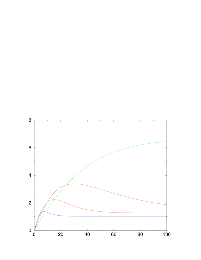
Figure 3: The dynamical susceptibility for the p-spin model (p=3) as a function of time for several temperatures the lower is the maximum the higher is the temperature. From bottom to top $T=1.0,0.9,0.8,0.7$.

As shown in ref. [9] we define $t^{*}$ as the time at which $\chi^{*}$ is maximum, we find that $\chi^{*}_{4}=\chi_{4}(t^{*})$ exhibit a divergence at $T_{c}$, as it is presented in figure 2. Both quantities behave as powers of $T-T_{c}$ $t^{*}\sim(T-T_{c})^{-\alpha}$, $\chi^{*}_{4}\sim(T-T_{c})^{-\gamma}$. A best fit gives the values $\gamma=0.52\pm 0.02$, $\alpha=1.1\pm 0.1$.

4 Conclusions

In this paper we have reviewed the analysis of the non linear susceptibility in supercooled liquids and glasses that comes from the mean field theory of disordered systems, and liquid models in the HNC approximation.

The theory predicts that while the long time, equilibrium susceptibility remains finite and is regular at all temperatures, the finite time susceptibility displays a maximum as a function of time which becomes higher and higher and displaced to larger and larger times for temperatures close to $T_{c}$. This behavior is a consequence of the critical character of the Mode Coupling like dynamical transition predicted by the ideal theory described in this paper. I real systems one can expect a similar behavion but with a round off of the divergence.

5 Acknowledgments

We thank C. Donati and S. Glotzer for many discussions on the topics of this paper.

6 References

References

- [1] W.Kob, C.Donati, S.J.Plimpton, P.H. Poole and S.C. Glotzer, Phys. Rev. Lett. 79 (1997) 2827. C. Donati, J.F. Douglas, W. Kob, S.J. Plimpton, P.H. Poole and S.C. Glotzer, Phys. Rev. Lett. 80 (1998) 2338.
- [2] Y. Hiwatari and T. Muranaka, J. Non-Cryst. Sol. 235-237, 19 (1998); D. Perera and P. Harrowell, ibid, 314.; A. Onuki and Y. Yamamoto, ibid, 34.
- [3] B. Doliwa and A. Heuer, Phys. Rev. Lett. 80, 4915 (1998).
- [4] C. Donati, S. C. Glotzer and P. H. Poole, Phys. Rev. Lett. in press.
- [5] C. Benneman, C. Donati, J. Baschnagel and S.C. Glotzer, Nature, 399, 246 (1999). See also p. 207.
- [6] C. Donati, S.C. Glotzer, P.H. Poole, W. Kob, and S.J. Plimpton, Phys. Rev. E 60 3102 (1999).
- [7] G. Parisi, J. Phys. Chem, 103(20), 4128 (1999).
- [8] S. Franz and G. Parisi, unpublished comment cond-mat/9804084.
- [9] C.Donati, S.Franz, G.Parisi, S.C. Glotzer, Theory of Non-linear Susceptibility and Correlation Length in Glasses and Liquids Preprint cond-mat/9905433
- [10] S.Franz, C.Donati, G.Parisi and S.C. Glotzer, Phyl. Mag. B 79 1827 (1999).
- [11] C. Dasgupta, A.V. Indrani, S. Ramaswami, and M.K. Phani, Europhys. Lett. 15 (1991) 307 [Addendum: Europhys. Lett. 15 (1991) 467].
- [12] S.C. Glotzer, V.N. Novikov, T.B. Schroeder preprint cond-mat/9909113
- [13] T.R. Kirkpatrick and P.G. Wolynes, Phys. Rev. A 35, 3072 (1987); T.R. Kirkpatrick and D. Thirumalai, Phys. Rev. B 36, 5388 (1987); T.R. Kirkpatrick and P. G. Wolynes, Phys. Rev. B 36, 8552 (1987).
- [14] M. Mezard and G. Parisi, J. Phys. A 29 65155 (1996).
- [15] W. Götze, Aspects of the Structural Glass Transition in Liquids, Freezing and the Glass Transition J.P. Hansen, D. Levesque, J. Zinn-Justin eds. North Holland 1990.
- [16] S. Franz and M. A. Virasoro Quasi-equilibrium interpretation of aging dynamics preprint cond-mat/9907438.
- [17] S. Franz and G. Parisi, J.Physique I 5 (1995) 1401; Phys. Rev. Lett. 79 (1997) 2486; Physica A 261, 317 (1998).
- [18] M. Cardenas, S. Franz, G. Parisi, J.Phys. A: Math. Gen. 31 L163 (1998); J. Chem. Phys. 110, 1726 (1999).
- [19] A review of the -spin model can be found in A. Barrat cond-mat/9701031 (unpublished).
- [20] A. Crisanti, H. Horner and H.J. Sommers, Z. Phys. B 92, 257 (1993).
- [21] S. Franz and M. Mezard, Physica A 210 (1994) 48.