Thermostatistics of extensive and non–extensive systems using generalized entropies

Abstract

We describe in detail two numerical simulation methods valid to study systems whose thermostatistics is described by generalized entropies, such as Tsallis. The methods are useful for applications to non-trivial interacting systems with a large number of degrees of freedom, and both short–range and long–range interactions. The first method is quite general and it is based on the numerical evaluation of the density of states with a given energy. The second method is more specific for Tsallis thermostatistics and it is based on a standard Monte Carlo Metropolis algorithm along with a numerical integration procedure. We show here that both methods are robust and efficient. We present results of the application of the methods to the one–dimensional Ising model both in a short–range case and in a long–range (non–extensive) case. We show that the thermodynamic potentials for different values of the system size $N$ and different values of the non–extensivity parameter $q$ can be described by scaling relations which are an extension of the ones holding for the Boltzmann–Gibbs statistics ($q=1$). Finally, we discuss the differences in using standard or non–standard mean value definitions in the Tsallis thermostatistics formalism and present a microcanonical ensemble calculation approach of the averages.

1 Introduction

Non–extensive systems are those for which the thermodynamic potentials do not scale linearly with the system size. As a way of example, in some electric or magnetic systems with very long–range interactions the ground state energy per particle increases with the number of particles. In the absence of other effects, such as screening, these system are “genuinely” non–extensive. If we apply to them the standard Boltzmann–Gibbs formalism of the Statistical Mechanics, we find that the internal energy, Helmholtz free energy and other thermodynamic potentials are non–extensive as well. This standard formalism can be implemented by using the definition of the entropy $S$ in terms of the probabilities $p_{i}$ of the $i=1,\dots,W$ possible microscopic configurations:

$$S=-\sum_{i}p_{i}\ln p_{i}$$ (1)

The actual calculation of the entropy assumes a set of probabilities $\{p_{i}\}$. These are computed by finding the maximum of the above expression when some extra conditions defining an ensemble (fixed number of particles and mean energy, for example) are imposed.

Even for systems in which the energy levels do scale with the system size, it is possible, by using generalized definitions of the entropy, to obtain non–extensive thermodynamic potentials. One of the most successful generalizations is that of Tsallis which in 1988 proposed [1] the following alternative expression for the entropy:

$$S_{q}=\frac{1-\sum_{i}p_{i}^{q}}{q-1}$$ (2)

where $q$ is an entropic index that characterizes the degree of non–extensivity. It is possible to show that the entropy of the composed system A+B satisfies the relation:

$$S_{q}(A+B)=S_{q}(A)+S_{q}(B)+(1-q)S_{q}(A)S_{q}(B)$$ (3)

when A and B are independent systems in the sense that $p_{ij}(A+B)=p_{i}(A)p_{j}(B)$. We see that for $q\neq 1$ there is no additivity in the entropy, which also implies non–extensivity. The Boltzmann–Gibbs entropy, Eq. (1), and extensivity are recovered in the limit $q\to 1$. Since the probabilities $\{p_{i}\}$ satisfy $p_{i}^{q}>p_{i}$ for $q<1$ and $p_{i}^{q}<p_{i}$ for $q>1$, the superextensive, $q<1$, and the subextensive, $q>1$, regimes will privilege the rare and frequent events respectively.

In the last years there have been many studies in which Tsallis non–extensive statistics has been applied to different situations (See [2, 3] for a review). In some cases, the systems considered are genuinely non–extensive (in the sense defined above) while in others the non–extensivity arises as a result of the application of the new statistics. In fact, and due to the intrinsic non–extensivity of the Tsallis statistics, it has been argued that its natural range of applicability should include systems with long–range interactions or long–range microscopic memory processes, as well as dynamical systems in which the space–time geometry has a multifractal–like structure, because those systems are in general genuinely non–extensive. Although most of the literature (including this paper) basically derives equilibrium properties starting from the generalized definition of the entropy, it has been conjectured recently [3], however, that the Tsallis entropy could be relevant instead in the study of non–equilibrium processes.

Due to the difficulty of deriving exact results, it is natural to use numerical methods to obtain the properties of a system with many degrees of freedom when studied under the rules of the new statistics. This is necessary in order to extract results that could be checked against experiments. However, these studies have been hampered by the failure of the typical Monte Carlo methods to adequately generate representative equilibrium configurations distributed according to Tsallis statistics. It is the purpose of this paper to explain in detail new methods that can be used to study the equilibrium properties of a many–particle system when it is considered under generalized statistics. Although our methods are quite general, we will illustrate their use by considering a prototypical genuinely non–extensive system: the Ising ferromagnet model with long–range interactions. We will also consider the short–range Ising model in order to test the simulation methods and to compare the results obtained from the use of Tsallis statistics in extensive and non–extensive systems.

In the remaining of the section, we will outline briefly which are the basic difficulties one encounters when trying to generalize the standard Monte Carlo methods (such as the Metropolis algorithm) to the study of Tsallis statistics. The main problem is that the probabilities $\{p_{i}\}$ can not be given an explicit expression, as we will see in the following discussion. Let us consider the canonical ensemble. The probabilities $\{p_{i}\}$ in this ensemble are found by solving the maximization problem of the entropy $S_{q}$ as given by Eq.(2) subject to the constrains of (i) positivity: $p_{i}\geq 0$, (ii) normalization: $\sum_{i}p_{i}=1$ and (iii) a fixed mean value for the internal energy: $\langle{\cal H}\rangle=U$, where $\cal H$ is the Hamiltonian of the system and the mean value of any function $O$ of the microscopic configurations is computed according to the general rule:

$$\langle O\rangle=\sum_{i}O_{i}u(p_{i}),$$ (4)

$O_{i}$ is the value of $O$ at the configuration whose probability is $p_{i}$ and we have introduced a function $u(p_{i})$ that allows the definition of generalized mean values. The standard mean values are recovered by taking $u(p_{i})=p_{i}$. Although, initially, the choices $u(p_{i})=p_{i}$ (first option), and $u(p_{i})=p_{i}^{q}$ (second option) were considered, later, it was shown that a better choice, in the sense that it preserves the Legendre structure of the resulting thermodynamics formalism, is to consider $u(p_{i})=p_{i}^{q}/\sum_{j}p_{j}^{q}$ (third option) [4]. We will use the following notation of the averages in this third option:

$$\langle O\rangle_{q}=\sum_{i}O_{i}P_{i}~{};~{}~{}~{}~{}~{}~{}~{}~{}~{}~{}P_{i}=\frac{p_{i}^{q}}{\sum_{j}p_{j}^{q}}.$$ (5)

$\{P_{i}\}$ are known as the “escorts” probabilities [5]. It is possible to recover the configuration probabilities $p_{i}$ from the escorts probabilities using:

$$p_{i}=\frac{P_{i}^{1/q}}{\sum_{j}P_{j}^{1/q}}.$$ (6)

The entropy, in terms of the $\{P_{i}\}$’s is given by:

$$S_{q}=\frac{1-(\sum_{i}P_{i}^{1/q})^{-q}}{q-1}$$ (7)

Concerning the different definitions for the averages, it should be said that it has been shown recently [6, 7, 8] that the standard mean values of the first option, $u(p_{i})=p_{i}$, can be also made compatible with the Legendre structure of the thermodynamics and the resulting formalism also represents a thermodynamically stable description. In this paper, we follow mainly the formulation in terms of the mean values defined by Eq.(5), although in a later section we will show that the results obtained using the standard mean values can be mapped onto the ones obtained using Eq. (5).

The maximization problem for the unknown escort probabilities $P_{i}$ in the canonical ensemble with a given internal energy $U_{q}$ is:

$$\frac{\delta~{}~{}}{\delta P_{i}}\bigl{[}S_{q}-\beta\sum_{i}\varepsilon_{i}P_{i}-\alpha\sum_{i}P_{i}\bigr{]} = 0$$ (8)

$$P_{i} \geq 0$$ (9)

$$\sum_{i}P_{i} = 1$$ (10)

$$\sum_{i}\varepsilon_{i}P_{i} = U_{q}$$ (11)

where $\alpha$, $\beta$ are Lagrange multipliers. $\{\varepsilon_{i}\}$ are the energy levels of the system under consideration whose ground state energy will be denoted by $E_{0}$. Solving the problem Eq.(8-11) one obtains the probabilities for the canonical ensemble as [4]:

$$P_{i}=\left\{\begin{array}[]{lr}0,&1-\frac{(1-q)\beta(\varepsilon_{i}-U_{q})}{(\sum_{j}P_{j}^{1/q})^{q}}<0\\ \frac{[1-(1-q)\beta(\varepsilon_{i}-U_{q})/(\sum_{j}P_{j}^{1/q})^{q}]^{\frac{q}{1-q}}}{\sum_{k}[1-(1-q)\beta(\varepsilon_{k}-U_{q})/(\sum_{j}P_{j}^{1/q})^{q}]^{\frac{q}{1-q}}},&{\rm otherwise}\end{array}\right.$$ (12)

The probabilities defined in this way are real and non–negative. The condition giving the possible values of $\beta$ and $\varepsilon_{i}$ for which $P_{i}\neq 0$ in Eq. (12) is called the cut–off condition. One can show that the probabilities Eq. (12) are invariant under a change in the energy levels $\varepsilon_{i}\to\varepsilon_{i}+\Delta\varepsilon$ (and the same change in the internal energy $U_{q}\to U_{q}+\Delta\varepsilon$) for arbitrary $\Delta\varepsilon$. By introducing the temperature $T=1/\beta$, it is possible to show also the validity of the relation [7, 4]

$$1/T=\partial S_{q}/\partial U_{q}$$ (13)

which reflects the Legendre structure of the thermodynamics obtained.

Notice that Eq.(12) does not give yet the actual values of the probabilities since the $\{P_{i}\}$’s appear in a non–trivial way in both sides of the equation (either explicitly or in the cut-off condition). This is different from the solution obtained in the usual Boltzmann–Gibbs canonical ensemble (recovered in the limit $q\to 1$) in which the solution adopts the explicit form:

$$P_{i}=\frac{{\rm e}^{-\beta\varepsilon_{i}}}{\sum_{j}{\rm e}^{-\beta\varepsilon_{j}}}$$ (14)

(although, of course, it is very difficult to compute the denominator of this expression, the partition function, for an interacting system). An iterative method to solve Eq.(12) has been used in [4]. In this method, an initial guess for the probabilities is fed in the right hand side of (12) and this equation is used recursively until convergence is achieved. We will see, however, that for many–particle systems, it might very difficult to achieve convergence in some cases.

A convenient way of writing Eq. (12) is by using an auxiliary parameter $\beta^{\prime}$ defined as [4]:

$$\beta^{\prime}=\frac{\beta}{(1-q)\beta\sum_{j}\varepsilon_{j}P_{j}+(\sum_{j}P_{j}^{1/q})^{-q}}$$ (15)

Defining $T^{\prime}\equiv 1/\beta^{\prime}$, and using Eqs. (7) and (11) one can rewrite this equation as

$$T=\frac{T^{\prime}-(1-q)U_{q}}{1+(1-q)S_{q}}$$ (16)

In terms of $\beta^{\prime}$ the solution adopts a form similar to that of the standard canonical ensemble:

$$P_{i}=\left\{\begin{array}[]{lr}0,&1-(1-q)\beta^{\prime}\varepsilon_{i}<0\\ \frac{[1-(1-q)\beta^{\prime}\varepsilon_{i}]^{\frac{q}{1-q}}}{\sum_{j}[1-(1-q)\beta^{\prime}\varepsilon_{j}]^{\frac{q}{1-q}}},&{\rm otherwise}\end{array}\right.$$ (17)

One can then adopt the following practical procedure [4]: choose a value for the parameter $T^{\prime}$ and compute the probabilities $P_{i}$ as a function of $T^{\prime}$ using Eq.(17). Compute the internal energy $U_{q}$, the entropy $S_{q}$ and the temperature $T$, always as a function of $T^{\prime}$, using Eqs. (11), (7) and (16), respectively. Finally, vary $T^{\prime}$ in order to make the parametric plots $U_{q}(T)$ and $S_{q}(T)$. Other thermodynamic potentials follow the usual definition. For instance, the Helmholtz free energy is $F_{q}=U_{q}-TS_{q}$.

It is important to realize that although the probabilities $P_{i}$, when considered as a function of $T$, do not depend on an arbitrary shift $\Delta\varepsilon$ of the energy levels or, in other words, do not depend on the zero of energy, $E_{0}$, they do depend on $E_{0}$ when considered as a function of $T^{\prime}$. This means that the averages as a function of $T^{\prime}$ can not be physically relevant because they depend on the zero of energy. This is why $T^{\prime}$ has to be interpreted only as an auxiliary parameter, not as an actual temperature. Of course, the relation $T^{\prime}\to T$ depends also on the zero of energy in such a way that both dependences cancel and the averages as a function of $T$ are independent of a shift in the energy levels. An interesting question is to determine the range of values for the parameter $T^{\prime}$ that should be used in order to obtain the usual range $0\leq T<\infty$ for the temperature $T$. Using that, according to the definition (2), it is $1+(1-q)S_{q}>0$ we obtain from Eq.(16) that $T^{\prime}$ should vary in the range $[(1-q)E_{0},\infty)$, where we have used that the energy at zero temperature is the ground state energy $U_{q}(T=0)=E_{0}$. Therefore, it is important to use the right range of values for $T^{\prime}$ in order to reach all the possible values for $T$. In particular, $T^{\prime}$ might need to take negative values either for $q<1$ or for $q>1$ unless one adopts $E_{0}=0$ as we will throughout this paper. To our understanding, it is not clear in the literature the fact that the averages as a function of the parameter $T^{\prime}$ depend on the zero of energy and that it might be necessary to consider negative values for $T^{\prime}$ in order to span the whole range of values for $T$.

As stated before, the main problem to perform Tsallis thermostatistics simulations at a given temperature $T$ is that there is not an explicit expression for the probabilities $P_{i}$, c.f. see Eq. (12). The practical procedure outlined above (compute $P_{i}$ as a function of $T^{\prime}$ and then compute $U_{q}$, $S_{q}$ and $T$ as a function of $T^{\prime}$ in order to make parametric plots by varying $T^{\prime}$) is not straightforward to implement numerically since it is very difficult to use Eq.(7) to compute the entropy. This is because the usual Monte Carlo methods, i.e. the Metropolis algorithm, require only the probabilities $P_{i}$ up to a normalization factor where Eq.(7) requires the absolute, normalized values of $P_{i}$. It is the object of this paper to explain in detail some numerical methods of the Monte Carlo type that can be used to perform the necessary averages for generalized statistics, including Tsallis.

There have been previous attempts to perform numerical simulations of Tsallis statistics using Monte Carlo methods. An earlier work in this direction is that of T. Penna et. al. [9] who extended the Metropolis acceptance procedure to include a dependence in the $q$ parameter. However, this method does not satisfy the detailed balance condition which is a key ingredient of Monte Carlo methods. Another interesting approach is that of I. Andricioaei et. al. [10], who performed a Metropolis Monte Carlo algorithm which does satisfy the detailed balance condition for the probability $P_{i}$ as a function of the parameter $T^{\prime}$ but, since they do not make the temperature transformation $T^{\prime}\to T$, they are unable to determine the actual temperature $T$ of the simulation. All these works considered the second version, $u(p_{i})=p_{i}^{q}$, for the definition of averages, which, as discussed before, has proven afterwards not to be the optimal election [4]. We have used also a similar sampling in the context of Simulated Annealing [11, 12]. A recent approach proposed by A. R. Lima et. al. [13] uses the broad histogram Monte Carlo method, which determines the number of microstates using a balance equation between near neighbor energy levels. They are able to apply this method to the Ising Model with short–range interactions. This is a valid Monte Carlo simulation with full control of the temperature $T$ but its applicability is somewhat restricted. As we will show, the Ising model with long–range interactions can not be treated straightforwardly with this method because the spin flip dynamics does not produce transitions between near energy levels and, consequently, the broad histogram Monte Carlo method, in its present form, can not be used to study long–range interacting systems. We are able to overcome these difficulties by extending a method which had been developed some time ago [14, 15, 16, 17] to compute directly the number of states with a given energy and which does not depend on the definition of the entropy. In fact, our method can be used to study any statistics and applications will be shown both for the Boltzmann–Gibbs and the Tsallis statistics. We develop yet a second method which is devised specifically for the Tsallis statistics and that has the advantage that it uses the familiar Metropolis algorithm plus a numerical integration.

This paper is organized in the following form: in section 2 we use a simple and limited enumeration procedure valid only for small system sizes. However, this method is exact and can be used to check against some of the approximated methods we will introduce later. In this section we also introduce the short–range Ising model (SRIM) and the long–range Ising Model (LRIM). These two models will be employed in this paper in order to test the numerical methods described here and to compare the behavior of the non–extensive Tsallis thermostatistics in genuinely extensive and non–extensive systems. In section 3 we explain in some detail the Histogram by Overlapping Windows (HOW) method. We show that this method has a wide range of applicability since it can be used both for short–range and long–range systems as well as for any kind of statistics. Section 4 presents a Metropolis Monte Carlo type method specially devised to study systems in the Tsallis statistics. In section 5 we present some results concerning the validity of some scaling relations for the SRIM and LRIM in the Tsallis thermostatistics context. These scaling relations are an extension of the ones holding for the Boltzmann–Gibbs statistics . In section 6 we present results for these models using standard mean values instead of those defined by Eq. (5). In section 7 we discuss the results of using Tsallis statistics in the microcanonical ensemble. Finally, in section 8 we summarize the main conclusions of this work.

2 Exact enumeration

The problem to compute the probabilities $\{P_{i}\}$ using Eq.(17) is that the number of terms in the sum of the denominator of this equation, the number of microstate configurations $W$, is extremely large (typically scales exponentially with the system size). However, for small systems, it might be possible to enumerate completely the microstates and, therefore, to compute magnitudes of interest such as the internal energy $U_{q}(T)$, the entropy $S_{q}(T)$, the free energy $F_{q}(T)$, etc. We follow this approach in this section. Although the system sizes one can usually study with this method are very far from reaching a situation in which scaling laws with system size apply, we use the results as a bench-test in order to compare with other approximate methods that will be introduced in the following sections.

We will consider Ising type models with Hamiltonian:

$${\cal H}=\sum_{(i,j)}J_{ij}({1-s_{i}s_{j}})$$ (18)

where each of the $N$ spin variables $s_{i}$, $i=1,\dots,N$ can take the values $\pm 1$. The sum $\sum_{(i,j)}$ runs over all distinct pairs of sites on a $d$-dimensional regular lattice of linear size $L=N^{1/d}$ with periodic boundary conditions and lattice constant equal to $1$. $J_{ij}$ is the coupling parameter between spins $i$ and $j$. Note that for ferromagnetic couplings, $J_{ij}\geq 0$, the ground state is double degenerate and its energy is $E_{0}=0$. The usual, nearest–neighbors, or short–range Ising model (SRIM), is obtained taking $J_{ij}=1$, if $r_{ij}=1$ and $J_{ij}=0$, if $r_{ij}>1$. The long–range Ising model (LRIM) is defined by using

$$J_{ij}=1/r_{ij}^{\alpha},$$ (19)

where $r_{ij}$ is the distance between the spins $i$ and $j$, and the parameter $\alpha$ sets the interaction range. The SRIM is formally recovered by taking the limit $\alpha\to\infty$. Depending on the value of $\alpha$ and the space dimension $d$, the LRIM has two regimes: the extensive regime, $\alpha>d$, and the non–extensive regime, $\alpha\leq d$. This can be seen by roughly estimating the mean energy per spin in an infinite system as $\int_{1}^{\infty}drr^{d-1}r^{-\alpha}$. We obtain a convergent integral if $\alpha>d$ (extensive behavior), and for $\alpha\leq d$ the integral diverges (non–extensive). More precisely, a convenient scale for the mean energy per spin in a finite system of size $N$ is given by [18]:

$$\tilde{N}=1+d\int_{1}^{L}drr^{d-1}r^{-\alpha}=\frac{N^{1-\alpha/d}-\alpha/d}{1-\alpha/d}$$ (20)

The definition of $\tilde{N}$ is such that the limit $\alpha\to d$ is well defined. Again, we see that for $\alpha>d$ the internal energy per spin scales as a constant in the limit of large $N$, but for $\alpha\leq ad$, it grows with the system size. The system is, in this latter case, genuinely non–extensive. The SRIM limit, $\alpha\to\infty$, gives the expected result $\tilde{N}=1$.

The number of configurations in the Ising model is $W=2^{N}$. We have made a complete enumeration of the $i=1,\dots,W$ configurations and their energies $\varepsilon_{i}$ for a linear chain, $d=1$, of sizes up to $N=34$. We have used these results to compute the probabilities $P_{i}$ and then the thermodynamic magnitudes of interest using Tsallis statistics with the third option for the averages. In Fig. 1, we plot the exact internal energy $U_{q}$ as a function of the temperature $T$, for several values of the parameter $q$ for the LRIM in a genuinely non–extensive situation, $\alpha=0.8$, Fig. 1.b, and for the SRIM, Fig. 1.a. In the $q<1$ case we observe that there is a range of temperatures for which the internal energy is not a single–valued function of the temperature and, for a given value of $T$, there are several possible values for $U_{q}$. This ambiguity is resolved by using a Maxwell–like construction [19, 4] that replaces the loop in the energy curves by a vertical straight line connecting the two points with the same free energy $F_{q}(T)$.

Figure 1: Internal energy $U_{q}$ as a function of the temperature $T$, from the exact evaluation of Eqs. (11,12) for one–dimensional Ising models with $N=34$ spins. Plot (a) is for the SRIM and plot (b) for the LRIM in a genuinely long-range case, $\alpha=0.8$. The insert shows the free energy $F_{q}$ for $q=0.6$. In this case, a part of the energy curve is replaced by a vertical straight line (shown by dots in the plot) such that the Maxwell criterion of equal free energies is satisfied.

Figure 2: The $T^{\prime}\to T$ transformation for the one–dimensional Ising models as obtained from the exact evaluation of Eq. (16) for a system size $N=34$ and different values of $q$. Plot (a) is for the SRIM, while plot (b) is for the LRIM for $\alpha=0.8$. Notice that, in both cases, there is a temperature range for which the curves are almost horizontal. This makes it very difficult to use iterative methods for the determination of the probabilities using directly Eq. (12).

We stress that the loops in the energy curves appear as a result of the $T^{\prime}\to T$ transformation and, therefore, will not be observed when plotting the energy as a function of $T^{\prime}$. Typical $T^{\prime}\to T$ transformations are shown in Fig. 2. We observe in this figure that for $q<1$ a same value of $T^{\prime}$ can correspond, in some cases, to three or more values of $T$ giving rise to the observed multivalued behavior in the energy. Figure 2 helps us to understand the failure of the iterative method that has been proposed [4] to solve the set of equations (12). Although each value of $T^{\prime}$ defines a unique set $\{P_{i}\}$. We see Fig. 2 that for $q>1$ there are some intervals of $T^{\prime}$ where the transformation $T^{\prime}\to T$ is almost horizontal. Therefore, one value of $T$ corresponds nearly to a complete interval for $T^{\prime}$ and hence, there are many possible solutions for $\{P_{i}\}$ very close to the real one. This is the main reason for the failure of iterative methods for $q>1$. The situation worsens for increasing system size $N$.

Whatever illuminating the method of exact enumeration is, its validity is limited to very small values for $N$. To our knowledge, the largest value ever considered in an exact enumeration scheme for a short–range Ising model is $N=4^{3}=64$ [20]. Simulations at larger $N$ sizes require other methods, as the ones presented in the next two sections.

3 The Energy Histogram Method using Overlapping Windows

Although the number of possible microscopic configurations is in general very large, the range of possible energy values usually takes a much smaller value. For instance, for the one–dimensional SRIM introduced in the previous section, with $N$ spins we have $W=2^{N}$, but the number of possible energy values is $N/2+1$. Let $M$, in general, be the number of possible energy levels. We denote by $\Omega(E_{k})$ the number of microscopic states sharing the same energy $E_{k}$, $k=0,\dots,M-1$. Obviously $\sum_{k}\Omega(E_{k})=W$. We rewrite all the sums in Eqs. (17,7,5) as:

$$P(E_{k}) = \left\{\begin{array}[]{lr}0,&1-(1-q)\beta^{\prime}E_{k}<0\\ \frac{[1-(1-q)\beta^{\prime}E_{k}]^{\frac{q}{1-q}}}{\sum_{n}\Omega(E_{n})[1-(1-q)\beta^{\prime}E_{n}]^{\frac{q}{1-q}}},&{\rm otherwise}\end{array}\right.$$ (23)

$$S_{q} = \frac{1-(\sum_{k}\Omega(E_{k})P(E_{k})^{1/q})^{-q}}{q-1}$$ (24)

$$\langle O\rangle_{q} = \sum_{k}\Omega(E_{k})O(E_{k})P(E_{k})$$ (25)

where the sums run over the $M$ energy levels.

Notice that, once the $\Omega(E_{k})$’s have been computed, any statistics can be performed upon the system. Whether we use Tsallis, Boltzmann–Gibbs or any other generalized statistics is simply a trivial change in the computational scheme. Moreover, it is also trivial to compute the averages for any value of the parameters, say $T$ or $q$. Therefore, although the calculation of the $\Omega_{k}$’s might be time consuming, the pay–off is tremendous.

In general, the $\Omega(E_{k})$ are very difficult to obtain exactly. An important exception that will be used throughout this paper is the SRIM in 1-d, for which the energy levels are given by $E_{k}=4k$ for $k=0,\dots,N/2$ and whose degeneracy is:

$$\Omega(E_{k})=2{N\choose{E_{k}/2}}$$ (26)

In the cases in which $\Omega(E_{k})$ is not known we need approximate numerical methods. The most naive way to find the $\Omega(E_{k})$’s is to generate different system configurations randomly and count how many times a configuration with energy $E_{k}$ appears. However, this approach fails because the complete set of $\Omega(E_{k})$ values span too many orders of magnitude. In general, two energy levels $E_{k}$ and $E_{n}$ could differ as much as $\Omega_{k}/\Omega_{n}\sim\exp{N}$. This means that the range of variation of $\Omega(E_{k})$ over the $M$ different energy levels is very large and it is not possible to generate in a single run a histogram that covers all the energy levels, unless one generates a number of configurations of the order of the total number available to the system, $W$.

The Histogram by Overlapping Windows method (HOW) used here [14] avoids this problem by generating system configurations within a restricted energy interval and estimating the relative weights of these energy levels from the number of times they appear in each interval. By generating enough intervals spanning the whole energy range, one is able to obtain good quality estimators of the numbers $\Omega(E_{k})$. An earlier account of the method has been given in [21] and we explain now in some detail how the method works.

Let us consider first the SRIM in arbitrary dimension. In this case, the possible energy values are $E_{k}=4k$ for $k=0,\dots,dN/2$. Following the original work [14], we consider the intervals (windows) $\{E_{0},E_{1},E_{2},E_{3}\}$, $\{E_{3},E_{4},E_{5},E_{6}\}$, $\{E_{6},E_{7},E_{8},E_{9}\}$, etc. Each window consists of $4$ consecutive energy levels and the last energy value of one window is the first of the next one. The next step is to take one of the intervals and to generate configurations whose energy belongs to it. This is achieved, after preparing the system initially with one of the energies of the interval, by flipping spins chosen at random. A spin flip is accepted only if it leaves the system in one of the energy levels of the interval and it is rejected otherwise. The ratio of the number of generated states with energy $E_{k}$ to the number of generated states with energy $E_{n}$ is an unbiased estimator of $\Omega(E_{k})/\Omega(E_{n})$, for $E_{k}$ and $E_{n}$ within the energy window. The quality of the estimator increases with the number of generated configurations. From the overlap between windows one can compute $\Omega(E_{k})$ for the whole range of energies. The number of energy values in each window ($4$ in the previous example) is not important as far as it is not too large (such that the ratios $\Omega(E_{k})/\Omega(E_{n})$ are not extremely small or large) and it is not too small either. If the window is very small, most spin flips will yield an energy outside the range of allowed values and the number of accepted, i.e. independent, configurations will be very small. Moreover, the final algorithm must be ergodic: any energy value in a window should be obtained from any other value in the same window after a sufficient number of spin flips.

Figure 3: The number of states $\Omega(E_{k})$ for $N=34$ calculated exactly (lines), and using the HOW method (symbols). (a) SRIM, (b) LRIM.

Figure 4: All the possible jumps from the energy level mark in black generated by a single spin flip. (a) SRIM, (b) LRIM. Note in (b) the small modulation in $\Omega(E_{k})$ of the order of $l_{E}=2\sum_{i=1}^{N}r_{ij}^{-\alpha}$ (See the text).

The same basic idea has been used in other short–range Hamiltonians [14, 15, 16, 17, 22]. We are concerned now with the extension of this method to consider long–range interactions, in particular the LRIM introduced before. A modification needed is that the energy values $E_{k}$ will represent now a continuum set of energies with a bin size $\delta E$. The energy levels are then $E_{k}=k\delta E$ $k=1,\dots,M$ and $\Omega(E_{k})$ counts all the configurations $i$ whose energy $\varepsilon_{i}$ satisfies $E_{k}\leq\varepsilon_{i}<E_{k}+\delta E$. In other words, one makes the approximation of considering that all the energies lying in one bin count as one single level. This turns out not to be a critical point, although one has to check that the results are independent, within the simulation errors, of the magnitude of $\delta E$.

Figure 5: The number of states $\Omega(E_{k})$ calculated using the HOW method for the 1–d Ising models for several values of $N$. (a) SRIM, (b) LRIM. In (b) we have shifted vertically the curves to avoid overlapping. The inserts show the collapse of all the curves using Eq. (27).

A more important point concerns the optimal size $l$ of the energy window $\{E_{k},E_{k+1},\dots,E_{k+l}\}$. Since, for a long–range interacting system, a single spin flip can produce a very large change in the energy, it is important not to choose $l$ too small. To make this point clear, we have calculated exactly the number of states $\Omega(E_{k})$ for a system with $N=34$ by using the complete enumeration of the $W=2^{34}$ possibles configurations, see Fig. 3. Using these exact results we study the energy changes that a single spin flip makes both in the SRIM and the LRIM cases. A typical situation is shown in Fig.4. In this figure we plot the histogram of the (exact) number of configurations using a value for the bin $\delta E=4$ for the SRIM, and $\delta E=1$ for the LRIM. We select several configurations belonging to one of the energy bins (marked black in the figure) and we dash all the levels that are obtained from these configurations by flipping one spin. We see that, as expected, the change in energy for the SRIM brings the system to one of its neighboring energy levels. However, for the LRIM the energy changes are very large and, in fact, the nearest–neighbor energy levels can not be reached by using the spin flip dynamics [23]. A measure of the typical change in energy obtained when flipping one spin is estimated by considering the ferromagnetic ground state configuration with all the spins pointing in the same direction. One spin flip in this configuration produces a change in energy $\Delta E=2\sum_{i=1}^{N}r_{ij}^{-\alpha}$. The equivalent number of energy bins is $\xi=\Delta E/\delta E$. We finally take the size of the energy windows $l=3\xi$. In order to make sure that ergodicity is satisfied, we adopt a large overlap of size $2\xi$ between the windows. This means that a window goes from $E_{k}$ to $E_{k+3\xi}$, but the next window goes from $E_{k+\xi}$ to $E_{k+4\xi}$ and so on. For the window $\{E_{k},E_{k+1},\dots,E_{k+3\xi}\}$ only those values in the interval $\{E_{k+\xi},\dots,E_{k+2\xi}\}$ are considered for the evaluation of the ratios $\Omega(E_{k})/\Omega(E_{n})$. To summarize, for the LRIM, it is necessary that both the window size and the overlap between windows has the correct size, depending on $\alpha$. For $\alpha=0.8$, used in our simulations, we take $\xi=4$ independently of the system size and adjust $\delta E$ accordingly. We have checked that $\xi=10$ gives the same results within the numerical errors. The number of configurations necessary increases with the required accuracy. We have adopted in our simulations the criterion that the minimum number of counts for any energy bin within a window is $100$. The knowledge of the exact degeneration of the ground state $\Omega(E_{0})=2$ allows finally the calculation of all the $\Omega(E_{k})$.

Figure 6: Internal energy $U_{q}(T)$ for 1–dimensional Ising models with $N=34$ and $q=0.8,1.0,1.2$. Symbols are obtained using the HOW method and lines show the exact results. (a) SRIM, (b) LRIM.

Figure 7: Internal energy $U_{q}$ as a function of temperature $T$ for one–dimensional Ising models and different values of $N$ and $q$, as coming from the application of the HOW method in the (a) SRIM and (b) LRIM. The values of $q$ are $q=0.8,0.9,1.0,1.1,1.2$ (curves from left to right).

In Fig. 3, we plot the number of states computed either exactly or by using the HOW method, for $N=34$ both for the SRIM and the LRIM. At the resolution of the figure, the exact results and the approximate ones are indistinguishable. This serves as a test that the HOW method, as implemented here, is capable or reproducing accurately the number of states in a known case. In Figs. 5, we show the number of states for sizes $N=34,100,200,400,1000$ as computed using the HOW method. The inserts of these figures show that this function scales as:

$$\Omega(E_{k})=\e^{N\phi(E_{k}/N\tilde{N})}$$ (27)

This is valid both for the SRIM and for the LRIM, if we recall that $\tilde{N}=1$ for the SRIM. The scaling function $\phi(x)$ is different for the SRIM and the LRIM. For the SRIM, the result (26) leads to:

$$\phi_{SRIM}(x)=\frac{x}{2}\ln\left(\frac{2}{x}-1\right)-\ln\left(1-\frac{x}{2}\right)$$ (28)

No analytical expression is available for the LRIM. Fig. 6 compares the result for the internal energy $U_{q}$ obtained using the HOW method and the exact results obtained from the exact enumeration algorithm in the case $N=34$. Again, we can see that differences are too small to show up in this plot. Finally, in Fig. 7 we make a similar plot for larger values of $N$ obtained in this case by application of the HOW method.

4 The Monte Carlo method

We have mentioned already that the usual Monte Carlo algorithms of the Metropolis type can not be applied to Tsallis statistics, because the probabilities $\{P_{i}\}$ are not known as a function of the temperature $T$. However, it is possible to use them to compute averages as a function of the parameter $T^{\prime}$ because the probabilities are known as a function of $T^{\prime}$ except for a normalizing factor, which is irrelevant in the Monte Carlo methods. Those averages can be performed by using the Metropolis algorithm to generate configurations distributed according to the probabilities $\{P_{i}\}$ as follows: consider the configuration $i$ with energy $\varepsilon_{i}$, flip a spin chosen at random to produce configuration $j$ with energy $\varepsilon_{j}$, accept this change with a probability $\min(1,P_{j}/P_{i})$. For the Boltzmann–Gibbs statistics the acceptance probability is the celebrated factor $\min[1,\exp(-\beta(\varepsilon_{j}-\varepsilon_{i}))]$. For Tsallis statistics, Eq. (17), it is instead:

$$P(i\to j)=\left\{\begin{array}[]{lr}0,&1-(1-q)\beta^{\prime}\varepsilon_{j}<0\\ \min\Biggl{[}1,\frac{1-(1-q)\beta^{\prime}\varepsilon_{j}}{1-(1-q)\beta^{\prime}\varepsilon_{i}}\Biggr{]}^{\frac{q}{1-q}},&{\rm otherwise}\end{array}\right.\\$$ (29)

This acceptance probability was used for the first time by I. Andricioaei et. al. [10]. After generating ${\cal N}$ configurations, the averages $\langle O\rangle_{q}$ at fixed $T^{\prime}$ are obtained as the sum: $\langle O\rangle_{q}={\cal N}^{-1}\sum_{s=1}^{\cal N}O(s)$, where $O(s)$ is the value of the observable $O$ at the configuration $s$ in the sequence of configurations generated by the Monte Carlo method.

Figure 8: The integration procedure implicit in the Eq. (32) to perform the $T^{\prime}\to T$ transformation in the Monte Carlo method. We use here $N=34$, $q=0.6$ and $T^{A}=0$. (a) SRIM, (b) LRIM.

Still, we need to perform the $T^{\prime}\to T$ transformation, in order to plot averages with respect to $T$, using Eq. (16). In this equation, we can use the Monte Carlo averages for the internal energy $U_{q}=\langle{\cal H}\rangle$, but the entropy is yet unknown. In order to compute the entropy, we combine Eq. (16) and Eq. (13):

$$\frac{\partial S_{q}}{\partial U_{q}}=\frac{1+(1-q)S_{q}}{T^{\prime}-(1-q)U_{q}}$$ (30)

which can be integrated between arbitrary points $A$ and $B$:

$$\frac{1}{1-q}\ln[1+(1-q)S_{q}]\biggr{|}_{A}^{B}=\int\limits_{U_{q}(A)}^{U_{q}(B)}\frac{dU_{q}}{T^{\prime}-(1-q)U_{q}}$$ (31)

to obtain:

$$S_{q}(B)=\frac{[1+(1-q)S_{q}(A)]\e^{\Bigl{[}(1-q)\int\limits_{U_{q}(A)}^{U_{q}(B)}\frac{dU_{q}}{T^{\prime}-(1-q)U_{q}}\Bigr{]}}-1}{1-q}$$ (32)

Figure 9: Internal energy $U_{q}$ as a function of the temperature $T$, for $N=34$ and $q=0.6$. By symbols we show the results of the Monte Carlo method and by lines the exact results. In the inserts we show the free energy criterion explained in the main text. (a) SRIM, (b) LRIM.

Finally, we need to know the value of the entropy, $S_{q}(A)$ at the initial integration point A. This depends on the particular system considered, but usually the extreme temperature cases are known. For the Ising models (both long–range and short–range), Eq. (18), the limits $T\to 0$ and $T\to\infty$ are:

• $S_{q}(T=0)=\frac{2^{(1-q)}}{1-q}$.

• $S_{q}(T=\infty)=\frac{2^{N(1-q)}}{1-q}$.

We have implemented this Monte Carlo method using a system size $N=34$. Fig. 8 shows that the function that needs to be integrated in order to perform the $T^{\prime}\to T$ transformation is a smooth one. Fig. 9 compares the internal energy obtained by this Monte Carlo method with the exact results obtained by the exact enumeration procedure showing the validity of this Monte Carlo scheme.

The main disadvantage of this Monte Carlo method is that one might need to simulate a large range of values of $T^{\prime}$ to be able to perform accurately the integration needed for the $T^{\prime}\to T$ transformation. However, the use of extrapolation techniques, such as the multiple histogram reweighting [24, 25], which permit to extend the results of a simulation at a value of the temperature to a continuum range of temperatures, allows to reduce dramatically the number of simulation points needed [21].

5 The scaling functions

For extensive systems, the internal energy per particle is just a function of the temperature, $U(N,T)/N=u(T)$. Clearly, by definition, this scaling relation does not hold for non–extensive systems and there has been some recent interest in finding the correct scaling laws that apply to non–extensive systems. A first result was to obtain the scaling laws that follow from the application of Boltzmann–Gibbs statistics to a genuinely non–extensive system such as the LRIM in the regime $\alpha<d$. The results for the internal energy, $U$, the magnetization $M$ (defined as $M=|\sum_{i=1}^{N}s_{i}|$ and computed using Eq. (25)), the Helmholtz free energy $F$ and the entropy $S$ can be summarized by the following relations [26, 27, 18, 28, 29, 30]:

$$U(N,T) = N\tilde{N}u(T/\tilde{N})$$ (33)

$$M(N,T) = Nm(T/\tilde{N})$$ (34)

$$F(N,T) = N\tilde{N}f(T/\tilde{N})$$ (35)

$$S(N,T) = Ns(T/\tilde{N})$$ (36)

where $m$,$u$,$f$,$s$ are the scaling functions. The argument justifying these scaling laws can be summarized as follows: the internal energy and the entropy appear in the definition of the free energy as $F=U-TS$, therefore one expects that $U$ and $TS$ should have the same behavior for large $N$. Since $U$ scales as $N\tilde{N}$ and $S$ scales as $N$ one obtains that $T$ must scale as $\tilde{N}$ thus leading to the previous scaling ansatzs. Note that the SRIM case is recovered from the LRIM case in the limit $\alpha\to\infty$, when $\tilde{N}\to 1$ and the scaling relations, Eq. (33-36), become the standard ones for extensive systems.

We present now the extensions of these scaling laws in the case that the models are considered under the rules of Tsallis entropy [22]. In the case $q\neq 1$, the entropy is no longer an extensive quantity (this is true both for the SRIM and the LRIM). In order to generalize the argument of the previous paragraph giving the correct scale factor for the temperature, we derive from Eq. (3) the following general expression for the entropy $A_{q}(N)$ of a set of $N$ independent particles:

$$A_{q}(N)=S_{q}(N,T=\infty)=\frac{[1+(1-q)S_{q}(1)]^{N}-1}{1-q}$$ (37)

here $S_{q}(1)$ is the one particle entropy. In the Ising model case, one particle can be in any of the two states with probability $1/2$, yielding: $S_{q}(1)=[1-2(1/2)^{q}]/(q-1)=[2^{1-q}-1]/(1-q)$. After replacing in Eq. (37), we obtain:

$$A_{q}(N)=\frac{2^{N(1-q)}-1}{1-q}$$ (38)

Assuming that Tsallis entropy will be scaled generically with $A_{q}(N)$, we now assume that $U$ and $TS$ scale in the same way as $N\tilde{N}$. Since $TS/N\tilde{N}=[TA_{q}(N)/N\tilde{N}][S/A_{q}(N)]$ we conjecture that the temperature has to be scaled with $N^{\prime}\equiv N\tilde{N}/A_{q}(N)$. However, it turns out that the numerical results do not support this expression for the rescaling factors in the case $q>1$. Therefore, we write the scaling relations in the following more general form:

$$U_{q}(N,T) = N\tilde{N}u_{q}(T/N_{U}^{\prime})$$ (39)

$$M_{q}(N,T) = Nm_{q}(T/N_{U}^{\prime})$$ (40)

$$F_{q}(N,T) = N\tilde{N}f_{q}(T/N^{\prime})$$ (41)

$$S_{q}(N,T) = A_{q}(N)s_{q}(T/N_{S}^{\prime})$$ (42)

The previous argument, valid in the case $q\leq 1$, implies simply $N^{\prime}_{U}=N^{\prime}_{S}=N^{\prime}$. For consistency in the notation, we define $A_{q}^{U}(N)$ and $A_{q}^{S}(N)$ by means of $N_{U}^{\prime}\equiv N\tilde{N}/A^{U}_{q}(N)$ and $N_{S}^{\prime}\equiv N\tilde{N}/A_{q}^{S}(N)$, respectively. Notice that for $q=1$ it is $A_{1}(N)\propto N$ and the scaling laws (33-36) are recovered. In order to obtain a good scaling description in the case $q>1$ it is seen numerically that one needs to assume the limits $A_{q}^{U}(N)\sim 2^{N(1-q)}/(q-1)$ and $A_{q}^{S}(N)\sim 2^{N(q-1)}/(q-1)$. A unifying expression that reduces to the necessary ones for large $N$ and for all values of $q$ is:

$$A_{q}^{S}(N)=\frac{2^{N(1-q)}}{q-1},\hskip 56.9055ptA_{q}^{U}(N)=\frac{A_{q}(N)^{2}}{A_{q}^{S}(N)}$$ (43)

Although we lack a satisfactory explanation for these relations, we note that similar scaling factors have been used previously to plot in the same scale curves for the specific heat in infinite–range Ising models and non–interacting ideal paramagnet [31, 32].

Figure 10: Internal energy $U_{q}(T)$ plotted in order to check the scaling relation Eq.(39) for $q=0.9,1.0,1.1$ and different system sizes. (a) SRIM, (b) LRIM.

Figure 11: Internal energy (top graph), magnetization (middle graph) and entropy (lower graph) plotted in order to check the proposed scaling relations Eqs. (39,40,42) for the short–range Ising model (SRIM). We have use $N=1000$ and the curves with $q<1$ include $q=0.2,\,0.4,\,0.6,\,0.8$ while the curves with $q>1$ include $q=1.2,\,1.4,\,1.6,\,1.8$. For clarity, in the entropy plot, the insert shows all the values of $q$, whereas the main plot shows only $q>1$.

Figure 12: Same plot that Fig. 11 but for the long–range Ising model (LRIM). We plot all the same $q$ values than in Fig. 11, although the different curves are almost indistinguishable with the resolution of this figure.

In order to check the validity of these scaling relations, we have used the HOW method to simulate the one-dimensional SRIM and LRIM with $\alpha=0.8$, for system sizes $N=34,100,200,400,800,1000$, and several values for the non–extensive parameter $q\in[0.1,1.9]$. We test the proposed scaling relations, Eq. (39-42), by plotting the scaled results in Figs. 10,11,12. One can observe in the Fig. 10 that, for the same value of $q$, the collapse of curves of different sizes $N$. This is similar to what has been observed in the $q=1$ case [27].

It is more remarkable the fact that, with the previous choice for the scaling factors, all the $q<1$ data collapse in a single curve. The same thing occurs for the $q>1$ curves. Therefore, data can be described by just three universal scaling functions, corresponding to $q<1$, $q=1$, and $q>1$ regimes respectively (See Figs. 11,12).

One can see in Figs. 11,12 that the collapse in the entropy curves for $q>1$ is very poor. This is easily understood by noticing that the low temperature limit of the entropy for infinite system size is $S_{q}(T=0)=(1-2^{1-q})/(q-1)$ whereas the high temperature limit is $S_{q}(T\to\infty)=1/(q-1)$ and those two finite values can not be rescaled simultaneously. This is different of what happens for the internal energy and the magnetization for which the limits $T\to 0$ and $T\to\infty$ coincide for different values of $q$. Finally, the scaling for the free energy follows directly from its definition $F_{q}=U_{q}-TS_{q}$. For $q\leq 1$ it is $f_{q}(x)=u_{q}(x)-xs_{q}(x)$, whereas for $q>1$ and in the limit of large $N$, the scaling function is given simply by $f_{q}(x)=u_{q}(0)-xs_{q}(\infty)=-x$.

In summary, the scaling laws given by Eqs. (39-42) work for all values of $q$ when using the scaling factors given by Eqs.(43). Moreover, the scaling functions $u_{q}$, $m_{q}$ and $f_{q}$ adopt only three different forms for each magnitude corresponding to $q>1$, $q=1$ and $q<1$, both in the SRIM and LRIM cases.

6 Thermostatistics using standard mean values

It has been shown recently [6, 7, 8] that the use of the standard rule for the calculation of the mean values in Tsallis statistics provides also a valid thermodynamical formalism. By “standard” rule we mean the use of the first option for the averages in which $u(p_{i})=p_{i}$ is used in (4). Moreover, it has been argued [4, 33] that the results of using this first option coincide with the results of the third option (the one used up to here in this paper) with a trivial change in the parameter $q\to 1/q$. In this section we show that it is possible indeed to map the results of one option into the results of the other, although the relation between them implies, besides the previous change in the parameter $q$, a non–trivial mapping for the temperature. Numerical results using the techniques developed in the previous sections, will allow us to plot the relation between the temperatures of the two options.

For the sake of clarity in the exposition we will use the subindexes “1” and “3” to denote the results one obtains in each option. Hence, the first option seeks the maximization of

$$S_{1}(q)=\frac{1-\sum_{i}p_{i}^{q}}{q-1}$$ (44)

subject to the canonical ensemble constrains: $p_{i}>0$, $\sum_{i}p_{i}=1$, $\sum_{i}\varepsilon_{i}p_{i}=U$. The third option, on the other hand, seeks the maximization of

$$S_{3}(q)=\frac{1-(\sum_{i}p_{i}^{1/q})^{-q}}{q-1}$$ (45)

subject to the same constrains. Of course, in the third option, the probabilities $p_{i}$ should be interpreted as “escort” probabilities, but this interpretation has no practical consequence whatsoever in the calculation of the averages. The key point now is that both entropies are related by:

$$S_{1}(1/q)=G_{q}[S_{3}(q)]$$ (46)

Figure 13: Transformation function between the two entropic forms $S_{3}(q)$ and $S_{1}(1/q)$ as indicated in Eq. (46).

Where $G_{q}(x)=\frac{q}{1-q}[1-(1+(1-q)x)^{-1/q}]$ is a monotonically increasing function of $x$. This function satisfies the property: $G_{q}^{-1}(x)=G_{1/q}(x)$, see Fig.(13). Hence, the same set of probabilities $\{p_{i}\}$ that maximize $S_{3}(q)$ for a given value of $U$ will maximize $S_{1}(1/q)$, for the same value for $U$. However, the fact that the probabilities coincide in both options does not mean that the averages computed using these probabilities coincide when they are plotted as a function of the temperature because it turns out that there is a non–trivial relation between the temperatures of both options. Let us denote by $T_{1}$ and $T_{3}$, respectively, the temperatures of the 1st and 3rd options. They can be defined as the (inverse of the) Lagrange multiplier needed to satisfy the constraint of fixed mean energy or, alternatively, they have been shown to satisfy the relations [7]:

$$1/T_{1}(q)=\frac{\partial S_{1}(q)}{\partial U}\hskip 56.9055pt1/T_{3}(q)=\frac{\partial S_{3}(q)}{\partial U}$$ (47)

Using (46) we find the desired relation between the two temperatures:

$$T_{3}(q)=T_{1}(1/q)/G^{\prime}_{1/q}[S_{1}(1/q)]$$ (48)

$G^{\prime}_{q}(x)$ is the derivative of $G_{q}(x)$. After substitution of Eq.(44), we find:

$$T_{3}(q)=T_{1}(1/q)(\sum_{i}p_{i}^{1/q})^{q+1}$$ (49)

Therefore, it is true that the results of the third option at the value $q$ of the parameter can be obtained from those of the first one at the value $1/q$. However, the mapping requires a non–trivial rescaling of the temperature, as given by Eq.(49). Let us recall again that only the dependence with $T$ does not vary when changing the zero of energies and, hence, can be the only physically relevant one.

Figure 14: The same plot as in Fig. (7) but using lineal mean values instead non–lineal ones for the values of $N$ indicated and $q=0.8,0.9,1.0,1.1,1.2$. (a) SRIM, (b) LRIM.

Figure 15: Transformation between temperatures $T_{1}$ and $T_{3}$ using Eq. (49) for $N=100$ and the indicated $q$ values. (a) SRIM, (b) LRIM.

In order to give an alternative explanation of the relation between the temperatures of both options, let us write down the solutions for the probabilities using the $\beta^{\prime}$ parameter. For the third option, the solution is read directly from Eq.(17) that we rewrite using the notation of this section:

$$p_{i}=\left\{\begin{array}[]{lr}0,&1-(1-q)\beta_{3}^{\prime}\varepsilon_{i}<0\\ \frac{[1-(1-q)\beta_{3}^{\prime}\varepsilon_{i}]^{\frac{q}{1-q}}}{\sum_{j}[1-(1-q)\beta_{3}^{\prime}\varepsilon_{j}]^{\frac{q}{1-q}}},&{\rm otherwise}\end{array}\right.$$ (50)

where the parameter $\beta^{\prime}_{3}=1/T^{\prime}_{3}$ is related to the temperature $T_{3}$ by Eq.(16) which reads:

$$T^{\prime}_{3}(q)=T_{3}(q)[1+(1-q)S_{3}(q)]+(1-q)U$$ (51)

For the first option, it is possible to write the solution in the following form:

$$p_{i}=\left\{\begin{array}[]{lr}0,&1-(1-1/q)\beta_{1}^{\prime}\varepsilon_{i}<0\\ \frac{[1-(1-1/q)\beta_{1}^{\prime}\varepsilon_{i}]^{\frac{1}{q-1}}}{\sum_{j}[1-(1-1/q)\beta_{1}^{\prime}\varepsilon_{j}]^{\frac{1}{q-1}}},&{\rm otherwise}\end{array}\right.$$ (52)

where the parameter $\beta^{\prime}_{1}=1/T^{\prime}_{1}$ is related to the temperature $T_{1}$ by [34]

$$T^{\prime}_{1}(q)=T_{1}(q)[1+(1-q)S_{1}(q)]+(1-1/q)U$$ (53)

Now, it is clear by comparing Eqs. (50) and (52) that the probabilities $p_{i}$ of the third option computed at $q$ are equal to the probabilities $p_{i}$ of the first option computed at $1/q$ provided that we choose the same values for the primed temperatures, $T^{\prime}_{3}(q)=T^{\prime}_{1}(1/q)$. After substitution of (51) and (53) and using (45), (44) we recover Eq.(49)

It is straightforward now to use the number of states $\Omega(E_{k})$ obtained using the HOW method to compute Eqs.(52,53,44) by replacing the sums over the configurations to sums over energy levels weighted by $\Omega(E_{k})$. In this way, we can perform the necessary averages implied in the first option as well as the temperature transformation factor needed in Eq. (49). In Fig. 14 we plot the internal energy $U_{q}$ as a function of the temperature using the standard averages of the first option. The most noticeable difference with the results of the third option, see figure (5) is that it is not necessary now to use the Maxwell construction because there are no loops with the temperature. In Fig. 15 we plot $T_{3}(q)$ vs. $T_{1}(1/q)$ in the LRIM and SRIM cases. Using these two results, it is possible to obtain the averages within the third option as a function of $T_{3}$. Of course, the results agree perfectly with those shown in Fig. 7. It is possible also to obtain from Eqs.(39-42) the scaling relations valid when the standard calculation of mean values is used for the calculation of thermodynamic quantitities.

7 Microcanonical Ensemble

As mentioned in the introduction, the third option can be formulated by using the entropic form Eq. (7) plus the standard rule for the calculation of mean values, Eq. (5) or, alternatively, by using the original entropic form Eq. (2), but with a mean value definition:

$$\langle O\rangle_{q}=\sum_{i}O_{i}\frac{p_{i}^{q}}{\sum_{j}p_{j}^{q}}.$$ (54)

These two points of view are completely equivalent. The first option, as explained in the previous section, uses also the original entropic form but with standard mean values. We will consider in this section Tsallis original entropic form $S(q)$ in the context of the microcanonical formalism. The aim is to be able to derive the internal energy without any a priori assumption about the definition of averages. In the microcanonical ensemble we consider the maximization problem for the original entropic form $S_{q}$ given by Eq.(2) with the constrain of given energy $E$. The solution is the equiprobability,

$$p_{i}=\left\{\begin{array}[]{lr}\Omega(E)^{-1},&\varepsilon_{i}=E\\ 0,&{\rm otherwise}\end{array}\right.$$ (55)

Where $\Omega(E)$ is the number of configurations with energy $E$. The entropy as a function of the energy is:

$$S_{q}(E)=\frac{\Omega(E)^{1-q}-1}{1-q}$$ (56)

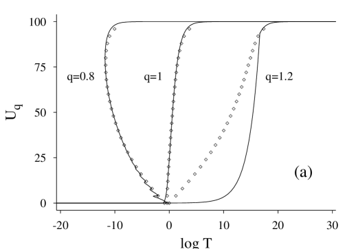
Figure 16: Plot of the internal energy as a function of the temperature for $N=100$. By points we show the results of using the microcanonical ensemble described in the text, and by lines the results obtained from the canonical ensemble (see Fig. 7) by using the non standard mean values of the third option. (a) SRIM, (b) LRIM.

The temperature is defined by the thermodynamic relation Eq. (13), $\frac{1}{T}=\frac{\partial S_{q}}{\partial E}$ or

$$\frac{1}{T}=\Omega(E)^{-q}\frac{\partial\Omega}{\partial E}$$ (57)

Inverting this relation, we obtain the energy as a function of the temperature, $E(T)$. In general, this relation needs to be inverted numerically. In terms of the scaling function $\phi(x)$ defined in (27) we have:

$$T=\frac{\tilde{N}\e^{(q-1)N\phi(E/N\tilde{N})}}{\phi^{\prime}(E/N\tilde{N})}$$ (58)

Figure 17: Plot of the energy fluctuations in the canonical ensemble $\sigma({\cal H)}/N\tilde{N}=\sqrt{\langle{\cal H}^{2}\rangle-\langle{\cal H}\rangle^{2}}/N\tilde{N}$ as a function of the scaled temperature for the indicated values of the sizes $N$ and the $q$ parameters. (a) SRIM, (b) LRIM.

where $\phi(x)$ is known exactly for the SRIM and can be evaluated numerically using the HOW method for the LRIM (from the plot in the insert of Fig. 5b). Results are shown in Fig 16 where we plot the internal energy coming from the application of the microcanonical ensemble to both the SRIM and the LRIM. In the same figure we have also plotted the energy coming from the canonical ensemble using non standard mean values (third option). We can see that both approaches coincide for $q\leq 1$, and differ for $q>1$ in some temperature range. The ultimate reason for not having equivalence between the two ensembles is that fluctuations of the energy in the canonical ensemble can not be neglected. We have checked that this is indeed the case by computing the energy fluctuations $\sigma({\cal H)}=\sqrt{\langle{\cal H}^{2}\rangle-\langle{\cal H}\rangle^{2}}$ as a function of the system size. In the Fig. (17) we see that fluctuations, normalized by the scale of energy, $N\tilde{N}$, do not decay to zero for increasing $N$ in the range of temperatures for which the microcanonical and canonical ensemble do not agree. For $q\leq 1$ fluctuations do decay to zero with the system size in all the temperature range.

If we compare the microcanonical and the canonical ensemble using the standard mean values (the first option studied in the last section) we observe the coincidence of both ensembles for $q\geq 1$, and disagreement (in a given temperature range) for $q<1$. This turns out to be also consistent with non–vanishing energy fluctuations in the appropriate range. This is the expected result because of the mapping $q\to 1/q$ implied in going from the third option to the first one.

8 Conclusions

In this paper, we have given details of two methods that can be used to perform numerical simulations for many particle systems that are governed by generalized statistics, such as the Tsallis one. The first method extends the Histogram by Overlapping Windows method, devised originally for short range Hamiltonians, to systems with very–long range interactions. The second method, devised specifically for the Tsallis thermostatistics, uses a typical Metropolis Monte Carlo updating scheme combined with a numerical integration. We have emphasized the need of using the right temperature definition if averages are to be independent of the zero of energy. We have applied our methods to the case of the Ising model with either short range (SRIM) or long range (LRIM) interactions. The latter case corresponds to a situation genuinely non–extensive in which the energy levels scale as $N^{\chi}$ with $\chi>1$, $N$ being the number of variables. We have compared the methods with some exact results available in the case of one–dimensional short range Ising model of arbitrary size and the long–range model for small system sizes.

We have shown that the internal energy, entropy, Helmholtz free–energy and magnetization follow non trivial scaling laws with the temperature $T$ and the number of variables $N$. We have justified these scaling laws by some heuristic arguments that, however, fail to reproduce the observed behavior for $q>1$. These scaling laws for $q\neq 1$ are non–extensive in the sense that the different thermodynamic potentials have to be scaled with a factor that depends in a non–trivial, i.e. non linear, way of $N$. The scaling laws hold for both the LRIM and the SRIM (with different scaling functions in each case), independently of the fact that the systems are genuinely non–extensive or extensive. This shows that the non–extensivity arises mainly because of the application of the Tsallis statistics.

We have discussed the differences between the use of standard (first option) and non–standard (third option) mean value definitions for the Tsallis Thermostatistics formalism. We show that, although the results of both definitions can be mapped onto each other by using the $q\to 1/q$ transformations, this mapping requires as well a non–trivial change in the temperature. Finally, we have shown that the use of the microcanonical ensemble coincides with the results of the canonical ensemble in the third option only for $q\leq 1$. We interpret this result as the non–vanishing energy fluctuations that occur in the corresponding case.

An obvious extension of the results presented here is to consider the Ising models in spatial dimension greater than one, [35]. The HOW method can be extended in any dimension for short range and long range interactions. For the SRIM in $d=2$ the exact results [36] should be used.

We remark that the present work concerns equilibrium systems and there is no time dependence in our simulations. However, it has been recently conjectured [3] that Tsallis statistics appears in some non–equilibrium systems such as the relaxation of the non–neutral plasma experiments in [37]. To study these non–equilibrium systems within the Tsallis statistics formalism, it would be more appropriate to use Molecular Dynamics (MD) methods in which the evolution equations are solved as a function of time. We are currently working on a MD simulation valid for a Lennard–Jones system within the Tsallis statistics. This MD method uses a Kusnezov, Bulgac and Bauer thermostat [38, 39] where additionally the actual temperature has to be calculated using a relation similar to the Eq. (32).

Acknowledgments

We wish to thank A.R. Plastino for several discussions about the Tsallis statistics and for useful suggestions. We acknowledge financial support from DGES, grants PB94-1167 and PB97-0141-C02-01.

References

- [1] C. Tsallis, Journal of Statistical Physics 52, 479 1988.
- [2] C. Tsallis, Physica A 221, 277 1995.
- [3] C. Tsallis, Braz. J. Phys. 29, 1 1999.
- [4] C. Tsallis, R.S Mendes, y A.R. Plastino, Physica A 261, 534 1998.
- [5] C. Beck y F. Schlgl, en Thermodynamics of chaotic systems. An introduction, Cambridge Nonlinear Science Series 4 Cambridge 1993.
- [6] R.S. Mendes, Physica A 242, 299 1997.
- [7] A. Plastino y A.R. Plastino, Physics Letters A 226, 257 1997.
- [8] G.R. Guerberoff y G.A. Raggio, J. Math Phys. 37, 1776 1996.
- [9] T.J.P. Penna, Physical Review E 51, R1 1995.
- [10] I. Andricioaei y J.E. Straub, Physical Review E 53, R3055 1996.
- [11] R. Salazar y R. Toral, Computer Physics Communications 121, 40 1999.
- [12] R. Salazar y R. Toral, Journal of Statistical Physics 89, 1047 1997.
- [13] A.R. Lima, J.S. Sá Martins, y T.J.P. Penna, Physica A 268, 553 1999.
- [14] G. Bhanot, R. Salvador, S. Black, P. Carter, y R. Toral, Physical Review Letters 59, 803 1987.
- [15] G. Bhanot, S. Black, P. Carter, y R. Salvador, Physics Letters B 183, 331 1987.
- [16] G. Bhanot, K. Bitar, S. Black, P. Carter, y R. Salvador, Physics Letters B 187, 381 1987.
- [17] G. Bhanot, K. Bitar, y R. Salvador, Physics Letters B 188, 246 1987.
- [18] P. Jund, S.G. Kim, y C. Tsallis, Physical Review B 52, 50 1995.
- [19] A.R. Lima y T.J.P. Penna, Phys. Lett. A 256, 221 1999.
- [20] R.B. Pearson, Phys. Rev. B 26, 6285 1982.
- [21] R. Salazar y R. Toral, Submitted to Physica A 1999.
- [22] R. Salazar y R. Toral, Phys. Rev. Lett. 83, 4233 1999.
- [23] This affirmation is valid for small values, which are needed in the method used in [13].
- [24] A.M. Ferrenberg y R.H Swendsen, Phys. Rev. Lett. 61, 2635 1988.
- [25] A.M. Ferrenberg y R.H Swendsen, Phys. Rev. Lett. 63, 1195 1989.
- [26] C. Tsallis, Fractals 3, 541 1995.
- [27] S.A. Cannas y F.A. Tamarit, Physical review B 54, R12661 1996.
- [28] L.C. Sampaio, M.P de Albuquerque, y F.S. de Menezes, Physical review B 55, 5611 1997.
- [29] J.R. Grigera, Physics Letters A 217, 47 1996.
- [30] H.H.A Rego, L.S. Lucena, L.R. da Silva, y C. Tsallis, Physica A 266, 42 1999.
- [31] F.D Nobre y C. Tsallis, Physica A 213, 337 1995.
- [32] F.D Nobre y C. Tsallis, Philosophical Magazine B 73, 745 1996.
- [33] G.A. Raggio, 1999, e–print cond–mat/9908207.
- [34] To prove this relation it is useful to consider the following identity: .
- [35] A study of the 2-d SRIM using the broad histogram Monte Carlo method was carried in [13]. .
- [36] P.D. Beale, Physical Review Letters 76, 78 1996.
- [37] X.P. Huang y C.F. Driscoll, Physical Review Letters 72, 2187 1994.
- [38] D. Kusnesov, A. Bulgac, y W. Bauer, Annals of Physics 204, 155 1990.
- [39] A.R. Plastino y C. Anteneodo, Annals of physics 255, 250 1997.