Hydrostatic theory of superfluid ³He-B

Abstract

The determination of the texture of the order parameter is important for understanding many experiments in superfluid ³He. In addition to reviewing the theory of textures in superfluid ³He-B we give several new results, in particular on the surface parameters in the Ginzburg-Landau region and bulk parameters at arbitrary temperature. Special attention is paid to separate the results that are valid at all temperatures from those which are limited to the Ginzburg-Landau region. We study the validity of a trivial strong-coupling model, where the energy gap of the weak-coupling theory is scaled by a temperature dependent factor. We compare the theory with several experiments. For some quantities the theory seems to work fine and we extract the dipole-dipole interaction parameter from the measurements.

I Introduction

The superfluid phases of liquid ³He show complex behavior, which still can be understood theoretically. Many phenomena have been studied in a pure form in ³He, and the knowledge can then be applied to other physical systems. For example, several structures of quantized vorticity have been seen in both A and B phases of ³He [1]. The effect of impurities has recently been studied in many laboratories by aerogel immersed in liquid ³He [2]. Recent experiments on the Josephson effect show unexpected behavior [3]. Theoretical understanding of all these phenomena requires good quantitative understanding of the basic properties of superfluid ³He. This provides the motivation for the present paper.

The purpose of hydrodynamics is to determine the behavior of a fluid on length and time scales that are long compared to some microscopic lengths and times [4]. Hydrostatics is a subfield of hydrodynamics. It is restricted to study the equilibrium properties of the fluid. In simple fluids hydrostatics reduces to statements about the pressure variation in the fluid, which either rotates uniformly or is exposed to some external field. The problem becomes more difficult, if the fluid has some broken symmetry. Particular examples of these are liquid crystals and superfluids ⁴He and ³He. In both superfluids, the equilibrium mass current belongs to the scope of the hydrostatic theory. The order parameter of ³He has also other degrees of freedom. The structure of those, which is often called texture, also has to be incorporated. In ³He the hydrostatic theory is limited to length scales that are large in comparison to the superfluid coherence length $\xi_{0}\approx 10\,$nm. The theory is valid at all temperatures. The hydrostatic theory can still be applied when the motion of the quasiparticles at low temperatures becomes ballistic rather than diffusive. The hydrostatic theory can be generalized to hydrodynamic theory by using conservation laws and adding the transport coefficients.

Our purpose is to make a systematic presentation of the hydrostatic theory for the B phase of superfluid ³He. Part of the reason is that presently the various results are scattered over a large literature. Previous reviews treat hydrostatics only as a side topic and cover only a small part of the subject [5, 6, 7, 8, 9, 10, 11]. The existing papers are often unclear whether they treat general temperatures or are restricted to the neighborhood of the superfluid transition temperature $T_{\rm c}$. We note that the hydrostatics of the A phase is better presented in the existing literature [6, 8, 9, 11] than the B phase considered here. In addition to reviewing, we present several results that have not been published before.

We will begin with a general formulation of the hydrostatics of ³He-B. Our approach is general enough to allow an external magnetic field and uniform rotation, both in the leading order. We write down an energy functional that consists of bulk terms and boundary conditions. All structures on the length scale of $\xi_{0}$, such as surface layer or vortex lines, have to be treated as boundary conditions. The theory is found to split into two pieces: one for the superfluid velocity and the other for the texture. The former is identical to the hydrostatics of superfluid ⁴He, whereas the latter can be solved only after the superfluid velocity is determined.

The coefficients of the hydrostatic energy can either be obtained experimentally or be calculated by some more microscopic theory. The calculation is discussed in sections III and IV. The former considers the quasiclassical theory of ³He [7]. The coefficients can be calculated using the weak-coupling quasiclassical theory at arbitrary temperature. We also discuss a “trivial strong-coupling” (TSC) model, where the weak-coupling coefficients are improved by scaling the energy gap. A different approach is studied in section IV, where the hydrostatic coefficients are related to the parameters of the phenomenological Ginzburg-Landau (GL) theory at $T\approx T_{\rm c}$.

Before any quantitative tests of the theory, we still have to determine the parameters that the quasiclassical theory needs as input. This is discussed in Section V, where we analyze several experiments. We find that certain quantities are reasonably well fitted using TSC model, but errors of 50% may occur for other quantities.

II Hydrostatic free energy

The superfluidity in a Fermi system arises from formation of Cooper pairs. A macroscopic number of pairs occupies the same pair state in the superfluid state [12]. The relative orbital wave function of a pair has p-wave symmetry in ³He and the spin state is a triplet [5, 13]. The state of the pairs is thus described by an order parameter, which is a complex $3\times 3$ matrix $A_{\alpha i}$. It gives the projections of the Cooper-pair wave function on the three p-wave orbitals ($p_{x}$, $p_{y}$, and $p_{z}$, index $i$) and on the three spin triplet states ($|-\uparrow\uparrow+\downarrow\downarrow\rangle$, ${\rm i}|\uparrow\uparrow+\downarrow\downarrow\rangle$, and $|\uparrow\downarrow+\downarrow\uparrow\rangle$, index $\alpha$). In unperturbed B phase the order parameter has the form

$$A_{\alpha j}=\Delta e^{{\rm i}\phi}R_{\alpha j}$$ (1)

with real $\Delta$, $\phi$ and $R_{\alpha j}$. Here the amplitude $\Delta$ has a fixed (temperature and pressure dependent) value and $R_{\alpha i}$ is constrained to be a rotation matrix, i.e. $R_{\alpha i}R_{\alpha j}=\delta_{ij}$. (Summation over repeated indices is assumed.) The phase $\phi$ and the more detailed form of the spin-orbit rotation matrix $R_{\alpha i}$ are not fixed on the scale of the superfluid condensation energy. These soft variables allow a dissipationless flow of both mass and spin. The order parameter can be interpreted as the wave-function of the center of mass of a pair. Using standard quantum mechanics, we can then define a mass-flow velocity

$${\bf v}_{\rm s}={\hbar\over 2m}{\mbox{\boldmath$\nabla$}}\phi,$$ (2)

where $m=5.0097\cdot 10^{-27}$ kg is the mass of a ³He atom. In a similar way one can also define a spin-flow velocity

$${\bf v}^{\rm spin}_{{\rm s},\alpha}=-{\hbar\over 4m}\epsilon_{\alpha\beta\gamma}R_{\beta i}{\mbox{\boldmath$\nabla$}}R_{\gamma i}\equiv{\hbar\over 4m}R_{\alpha i}\epsilon_{ijk}R_{\beta j}{\mbox{\boldmath$\nabla$}}R_{\beta k},$$ (3)

where $\epsilon_{ijk}$ is the maximally antisymmetric tensor. For example, if the axis of the spin-orbit rotation is constant and parallel to $z$, the pairs with spin states $|\uparrow\uparrow\rangle$, $|\downarrow\downarrow\rangle$, and $|\uparrow\downarrow+\downarrow\uparrow\rangle$ flow with velocities ${\bf v}_{\rm s}+{\bf v}^{\rm spin}_{{\rm s},z}$, ${\bf v}_{\rm s}-{\bf v}^{\rm spin}_{{\rm s},z}$, and ${\bf v}_{\rm s}$, respectively. The three-dimensional rotation matrices are conveniently parametrized by an angle $\theta$ and an axis $\hat{\bf n}$ of rotation as

$$R_{ij}(\hat{\bf n},\theta)=\cos\theta\delta_{ij}+(1-\cos\theta)\hat{n}_{i}\hat{n}_{j}-\sin\theta\epsilon_{ijk}\hat{n}_{k},$$ (4)

where $\hat{\bf n}\cdot\hat{\bf n}=1$. We note also the trivial identity $\hat{\bf a}\cdot\tensor{R}\cdot\hat{\bf a}=\cos\theta+(1-\cos\theta)(\hat{\bf a}\cdot\hat{\bf n})^{2}$, where $\hat{\bf a}$ is an arbitrary unit vector.

The soft variables $\phi$ and $R_{\alpha i}$ are determined by the interaction of the order parameter with various perturbations. The perturbations can be divided into external fields and boundary conditions. Experimentally, the most common field is the magnetic one ${\bf H}$. It would also be straightforward to include the electric field, but we will neglect it here because its coupling is very weak [14]. The motion of the ³He container can also be treated as an external field. In equilibrium the normal fluid component (velocity ${\bf v}_{\rm n}$) will follow the motion of the container, and the only allowed motions are uniform translation and rotation. The former is automatically taken into account because of Galilean invariance of the theory. The rotation will appear as a field $\nabla\times{\bf v}_{\rm n}$, which equals twice the angular velocity.

It is possible to construct a hydrostatic theory for any magnitude of the external fields. Here we assume the fields are small enough that the order parameter is not distorted strongly from the bulk form (1). Strong perturbations, such as a surface or a vortex core, are treated as boundary conditions. These cause the order parameter to deviate substantially from the bulk form within a length scale of the coherence length $\xi_{0}\approx 10$ nm, but on longer length scales also they act as weak perturbations.

The degrees of freedom $\phi$ and $R_{\alpha i}$ differ crucially in the following respect. The mass flow can be written as ${\bf j}_{{\rm s}}=\tensor{\rho}_{\rm s}\cdot{\bf v}_{{\rm s}}$, where $\tensor{\rho}_{\rm s}$ is a phenomenological tensor. In the absence of external fields, $\tensor{\rho}_{\rm s}$ must be a scalar because of the isotropy of the unperturbed $A_{\alpha i}$ (1). The mass current has also to be conserved: $\nabla\cdot{\bf j}_{\rm s}=0$. Thus we arrive at the Laplace equation $\nabla^{2}\phi=0$. Adding the boundary conditions, this completely determines $\phi$. The external fields cause only a small correction to this. Throughout the rest of this paper we neglect the small correction and start out from the assumption that the Laplace equation for $\phi$ is already solved, and thus ${\bf v}_{\rm s}$ is known.

The problem that remains is to determine the rotation matrix $R_{\alpha i}$. What makes this different from $\phi$ is that there exists interaction between the nuclear dipole moments of the ³He atoms. It is of the form [15]

$$F_{\rm D}=\lambda_{\rm D}\int d^{3}r(R_{ii}R_{jj}+R_{ij}R_{ji})=4\lambda_{\rm D}\int d^{3}r\cos\theta(1+2\cos\theta).$$ (5)

Although this interaction is weak, it partly removes the degeneracy with respect to the rotation matrix. This means that the spin current is not conserved, but decays on a scale $\xi_{\rm D}\approx 10\ \mu$m. On the same scale, the rotation angle $\theta$ becomes fixed to $\arccos(-1/4)\approx 104^{\circ}$, which corresponds to the minimum of $F_{\rm D}$ (5), but the degeneracy with respect to the rotation axis $\hat{\bf n}$ remains. Because no conservation laws exist, the rotation axis $\hat{\bf n}$ is more susceptible to all kinds of perturbations than $\phi$. The subject of the rest of this paper is to study the texture, i.e. $\hat{\bf n}({\bf r})$ on a length scale $\gg\xi_{\rm D}$.

We write down the free energy functional that governs the texture. The form of the energy terms is based on symmetry properties alone. The functional is valid in the limit of low fields and velocities, small gradients of the order parameter and weak coupling between the spin and orbital parts of the order parameter. The last condition is practically always satisfied because the coupling is due to the dipole-dipole interaction (5), which is small compared to the superfluid condensation energy by factor $10^{-6}(1-T/T_{c})^{-1}$. We neglect all constant terms, i.e. terms that do not depend on $\hat{\bf n}$. The leading terms in the expansion can be written as follows

$$F_{\rm DH}=-a\int d^{3}r(\hat{\bf n}\cdot{\bf H})^{2}$$ (6)

$$F_{\rm DV}=-\lambda_{\rm DV}\int d^{3}r[\hat{\bf n}\cdot({\bf v}_{\rm s}-{\bf v}_{\rm n})]^{2}$$ (7)

$$F_{\rm HV}=-\lambda_{\rm HV}\int d^{3}r[{\bf H}\cdot\tensor{R}\cdot({\bf v}_{{\rm s}}-{\bf v}_{{\rm n}})]^{2}$$ (8)

$$F_{\rm HV1}=-\lambda_{\rm HV1}\int d^{3}r{\bf H}\cdot\tensor{R}\cdot\mbox{\boldmath$\nabla$}\times{\bf v}_{{\rm n}}$$ (9)

$$F_{\rm G}=\int d^{3}r\left[\lambda_{\rm G1}{\partial R_{\alpha i}\over\partial r_{i}}{\partial R_{\alpha j}\over\partial r_{j}}+\lambda_{\rm G2}{\partial R_{\alpha j}\over\partial r_{i}}{\partial R_{\alpha j}\over\partial r_{i}}\right].$$ (10)

The dipole-field term $F_{\rm DH}$ is discussed in Refs. [16, 17], the gradient term $F_{\rm G}$ in Refs. [18, 17], the dipole-velocity $F_{\rm DV}$ and field-velocity $F_{\rm HV}$ in Ref. [6], and the first-order field-velocity term $F_{\rm HV1}$ in Ref. [19]. Because of Galilean invariance only the combination ${\bf v}_{\rm s}-{\bf v}_{\rm n}$ appears in Equations (7) and (8). The superfluid velocity does not appear in the gyromagnetic term (9) because ${\bf v}_{\rm s}$ is curl free. Terms that are linear in $\hat{\bf n}\cdot{\bf H}$, $\hat{\bf n}\cdot({\bf v}_{\rm s}-{\bf v}_{\rm n})$ or ${\bf H}\cdot\tensor{R}\cdot({\bf v}_{{\rm s}}-{\bf v}_{{\rm n}})$ are prohibited by parity and time-reversal symmetry. Equations (6)-(10) serve as definitions of the parameters $a$, $\lambda_{\rm DV}$, $\lambda_{\rm HV}$, $\lambda_{\rm HV1}$, $\lambda_{\rm G1}$ and $\lambda_{\rm G2}$, which depend on temperature and pressure. The calculation of these parameters are discussed in Sections III and IV. For some of the parameters we use names given in Ref. [17] instead of the more systematic names introduced here; for example $\lambda_{\rm DH}\equiv a$ and $\lambda_{\rm SH}\equiv d$.

The derivation of the gradient energy (10) deserves special consideration. Originally, one starts from a general expression that is quadratic in the spin velocity (3). Making use of the properties of the rotation matrices, it is possible to simplify the energy to a form that is bilinear in the rotation matrices $R_{\alpha i}$. In addition to the two terms in (10), this form contains a third term of the form $\partial_{i}R_{\alpha j}\partial_{j}R_{\alpha i}$. The form (10) can then be obtained by partial integration which converts the third term into the form $\partial_{i}R_{\alpha i}\partial_{j}R_{\alpha j}$.

It should be noted that the partial integration of the gradient energy (10) produces a surface term that is similar to $F_{\rm SG}$ below. Thus the value of the surface coefficient $\lambda_{\rm SG}$ is unique only if the form of the bulk gradient energy is properly defined. Here the uniqueness of $\lambda_{\rm SG}$ is guaranteed by restricting the bulk gradient energy to the form (10).

The gradient term can also be expressed explicitly as a function of $\hat{\bf n}$ using the representation (4) [17]. The needed identities are given in the Appendix. Our preference is to keep the shorter form (10) because a numerical algorithm can directly be based on it.

The dipole length $\xi_{\rm D}$ is defined by $\xi_{\rm D}=\sqrt{\lambda_{\rm G2}/\lambda_{\rm D}}$. It is conventional to define dipole velocity $v_{\rm D}$ and dipole field $H_{\rm D}$ by writing $\lambda_{\rm HV}=2a/(5v_{\rm D}^{2})$ and $\lambda_{\rm DV}=aH_{\rm D}^{2}v_{\rm D}^{-2}$. We can also define a magnetic coherence length $\xi_{\rm H}=\sqrt{65\lambda_{\rm G2}/(8aH^{2})}$, which is inversely proportional to the field. The parameters defined here are temperature dependent. Near $T_{\rm c}$ they reduce to constants that are commonly used. For example, $\xi_{\rm H}\rightarrow R_{\rm c}H_{\rm B}/H$ defined in Ref. [17].

In addition to the bulk terms (6)-(10), there are boundary terms. These energy terms originate from regions where the order parameter is strongly distorted from the form (1). We are here interested in two cases: surfaces and vortex cores. The boundary terms below are valid in the limit that the length scale of the distorted region ($\approx\xi_{0}$) is small compared to the dipole length $\xi_{\rm D}$. In reality this is well the case. It guarantees that the rotation angle $\theta$ is not affected by the boundary. The form of the allowed boundary terms depends on the symmetry of the order parameter at the boundary.

We assume that the surface structure has the maximal symmetry, i.e. time-inversion symmetry, rotation symmetry around the surface normal and reflection symmetry in planes perpendicular to the surface. (We note that also less symmetric states are possible [20].) We also assume that the curvature of the surface is small. Such a surface gives rise to the energy terms

$$F_{\rm SH}=-d\int_{S}d^{2}r({\bf H}\cdot\tensor{R}\cdot\hat{\bf s})^{2}$$ (11)

$$F_{\rm SHV1}=-\lambda_{\rm SHV1}\int_{S}d^{2}r{\bf H}\cdot\tensor{R}\cdot\hat{\bf s}\times({\bf v}_{{\rm s}}-{\bf v}_{{\rm n}})$$ (12)

$$F_{\rm SG}=\lambda_{\rm SG}\int_{S}d^{2}r\hat{s}_{j}R_{\alpha j}{\partial R_{\alpha i}\over\partial r_{i}}$$ (13)

$$F_{\rm SD}=\int_{S}d^{2}r[b_{4}(\hat{\bf s}\cdot\hat{\bf n})^{4}-b_{2}(\hat{\bf s}\cdot\hat{\bf n})^{2}].$$ (14)

Here $\hat{\bf s}$ is a unit vector that is perpendicular to the surface and points towards the superfluid. The surface-field term $F_{\rm SH}$ is discussed in Ref. [18, 17], the surface-dipole term $F_{\rm SD}$ in Ref. [18, 21, 17], and the first-order surface-field-velocity term $F_{\rm SHV1}$ in Ref. [19]. There are two contributions to the surface-gradient coefficient, $\lambda_{\rm SG}=\lambda_{\rm SG}^{\rm a}+\lambda_{\rm SG}^{\rm b}$. The former comes from the equilibrium spin current that flows spontaneously along any surface[22]. In fact, the surface spin current $J^{\rm ss}_{\alpha i}=\lambda_{\rm SG}^{\rm a}R_{\alpha j}\epsilon_{ijk}\hat{s}_{k}$. (Note that $J^{\rm ss}$ contains the factor $\hbar/2$ for each fermion and thus has the unit J/m.) The other contribution $\lambda_{\rm SG}^{\rm b}$ comes from the partial integration that depends on the chosen form of $F_{\rm G}$ [17]. Note that there exists only one surface-gradient term (13) because $R_{\alpha i}\nabla R_{\alpha j}$ is antisymmetric in $i$ and $j$. For the same reason the term (13) does not depend on the normal derivative. We have constructed the definitions (6)-(14) so that all surface ($d$, $\lambda_{\rm SHV1}$, $\lambda_{\rm SG}$, $b_{2}$, $b_{4}$) and bulk coefficients are non-negative, at least in the Ginzburg-Landau region.

The order parameter is strongly distorted from the bulk form (1) in the cores of quantized vortex lines. Therefore the cores must be treated as boundary regions. We describe a vortex line by unit vector $\hat{\bf l}$ that is parallel to the line and points in the direction of the circulation $\nabla\times{\bf v}_{\rm s}$. The maximal point-symmetry operations of a vortex are a) reflection in plane perpendicular to $\hat{\bf l}$, b) rotation around $\hat{\bf l}$ (combined with a phase shift) and c) reflection in plane containing $\hat{\bf l}$. The last one has to be combined with time inversion because otherwise the circulation would change direction. Assuming that the order parameter in the core has all these symmetries, we get the phenomenological terms

$$F_{\rm LH}=\lambda_{\rm LH}\int_{L}d^{3}r({\bf H}\cdot\tensor{R}\cdot\hat{\bf l})^{2}$$ (15)

$$F_{\rm LH1}=\lambda_{\rm LH1}\int_{L}d^{3}r{\bf H}\cdot\tensor{R}\cdot\hat{\bf l}$$ (16)

$$F_{\rm LD}=\lambda_{\rm LD}\int_{L}d^{3}r[(\hat{\bf l}\cdot\hat{\bf n})^{2}+\hbox{corrections}].$$ (17)

The line-field term $F_{\rm LH}$ is discussed in Ref. [23], the first-order line-field term $F_{\rm LH1}$ in Ref. [24], and line-dipole term $F_{\rm LD}$ in Ref. [25]. Here $L$ denotes the region where vortices are present. In $F_{\rm LD}$ only the dominant term is written explicitly.

It is well known that the vortex cores do not have the maximal symmetry [25]. In the A-phase-core vortex the symmetry (a) is broken. Because this can take place in two different ways, we have to assign to each vortex line a new variable $q$ that equals either +1 (left-handed vortex) or -1 (right handed vortex). This allows the line-gradient term [9]

$$F_{\rm LG}=\lambda_{\rm LG}\int_{L}d^{3}r\,\langle q\rangle\hat{l}_{j}R_{\alpha j}{\partial R_{\alpha i}\over\partial r_{i}},$$ (18)

where $\langle\ldots\rangle$ denotes the average because $q$ may change from one vortex to another. Similar to the surface term $F_{\rm SG}$, $F_{\rm LG}$ arises from spontaneous spin currents. For an isolated vortex these currents form closed loops in the plane perpendicular to $\hat{\bf l}$. All vortices in ³He-B also have axial spin currents but they do not couple to external spin velocity in the lowest order because the net current vanishes.

The double-core vortex also allows the term (18). Additionally, the circular symmetry (b) is broken leaving only discrete symmetry in rotations by $\pi$. Thus an additional unit vector $\hat{\bf b}$ perpendicular to $\hat{\bf l}$ is needed to describe the vortex. This gives rise to line-anisotropy terms

$$F_{\rm LAH}=\lambda_{\rm LAH}\int_{L}d^{3}r\langle({\bf H}\cdot\tensor{R}\cdot\hat{\bf b})^{2}\rangle$$ (19)

$$F_{\rm LAD}=\lambda_{\rm LAD}\int_{L}d^{3}r\langle(\hat{\bf b}\cdot\hat{\bf n})^{2}+\hbox{corrections}\rangle.$$ (20)

We note that there is flexibility in the definitions of the different terms. For example, the superflow around a vortex has to be counted into term $F_{\rm LH}$ (15) in the region where the order parameter is strongly distorted but at larger distances it also can be included as the bulk term $F_{\rm HV}$ (8).

III Connection to the quasiclassical theory

The energy terms (5)-(20) contain a number of phenomenological coefficients. They should either be determined experimentally or calculated from a more microscopic theory than the hydrodynamic one. Pursuing the latter, there exists the quasiclassical theory [7]. This theory bypasses the difficult many-body problem of strongly interacting ³He atoms by concentrating in the low-energy range. It uses an expansion, where the relevant expansion parameter for the superfluid phases is the transition temperature divided by the Fermi temperature, $T_{\rm c}/T_{\rm F}\sim 0.001$. The lowest nontrivial order in this expansion is known as the weak-coupling theory. It effectively contains the Bardeen-Cooper-Schrieffer theory as a special case, but it also reduces to the Landau Fermi-liquid theory in the normal state. This theory is adequate for some properties of superfluid ³He, especially at low pressures, but it fails, for example, to stabilize the A phase. For many purposes it is important to continue the expansion to the next order in $T_{\rm c}/T_{\rm F}$. We call this the strong-coupling theory. (Serene and Rainer use the name “weak-coupling plus”, but we think this is too modest since there seems to be very little hope to calculate further orders in the expansion.) We will not go into the details of the quasiclassical theory, which is extensively discussed by Serene and Rainer [7].

It is important to realize that the quasiclassical theory is not microscopic in the sense that it would depend only on fundamental constants. Instead, it needs several parameters as input. This is especially a problem in the strong coupling case, which needs as input the scattering amplitude of quasiparticles (in the normal state) that is not accurately known. Additionally, the needed calculations are rather complicated at general temperature. There are two practical ways to proceed. The first is to restrict to the temperature region close to $T_{\rm c}$ and use the Ginzburg-Landau theory. This approach will be described in Section IV. The second way is to work at arbitrary temperature but to use the weak-coupling approximation in the quasiclassical theory. The latter approach is discussed in this section. At the end of this section we discuss how to improve the weak-coupling results by including a trivial strong-coupling correction.

In the weak-coupling theory, the properties of the normal state are included via spin symmetric and antisymmetric Fermi-liquid parameters, $F_{l}^{\rm s}$ and $F_{l}^{\rm a}$ ($l=0$, 1, 2, $\ldots\infty$). We assume that the pairing interaction is effective in the p-wave channel only. The symmetry between particle and hole types of quasiparticles is consistently assumed in the quasiclassical theory. It turns out that all results presented below depend only on five Fermi-liquid parameters: $F_{1}^{\rm s}$ and $F_{l}^{\rm a}$ with $l=0$, 1, 2, and 3. (Infinite number of coefficients is needed in the hydrostatics of the A phase [26].) In addition, the results depend on the mass density $\rho$ of ³He liquid, on the superfluid transition temperature $T_{\rm c}$ and on the magnetic dipole-dipole interaction parameter $g_{\rm D}$.

In the Bardeen-Cooper-Schrieffer model $g_{\rm D}$ has the expression [15] (in SI units)

$$g_{\rm D}={\mu_{0}\over 40}\bar{R^{2}}\left(\hbar\gamma N(0)\pi k_{\rm B}T\sum_{\epsilon_{n}=-\epsilon_{\rm c}}^{\epsilon_{\rm c}}{1\over\sqrt{\epsilon_{n}^{2}+\Delta^{2}}}\right)^{2},$$ (21)

where $\bar{R^{2}}$ is a renormalization constant and $\epsilon_{\rm c}$ a high energy cut-off. (Note that our definition of $g_{\rm D}$ [8] is different from that in Ref. [15].) The Matsubara energies $\epsilon_{n}$ and the weak-coupling energy gap $\Delta(T)$ are defined in the Appendix, the gyromagnetic ratio of the ³He nucleus $\gamma=-2.04\cdot 10^{8}\ ({\rm T\ s})^{-1}$, and the density of states at the Fermi energy $2N(0)=(1+{1\over 3}F_{1}^{\rm s})(3m^{2}\rho/\pi^{4}\hbar^{6})^{1/3}$. It is very convenient that the dependence of $g_{\rm D}$ on temperature is so weak that we can safely ignore it. In the weak-coupling approximation the constancy of $g_{\rm D}(T)$ would be exact if the cut-off energy $\epsilon_{\rm c}$ in (21) were the same in the gap equation (54). (For the standard choice $\epsilon_{\rm c}\rightarrow\infty$ in the gap equation and $\bar{R^{2}}=1$, the relative variation of $g_{\rm D}(T)$ is less than $10^{-5}$.) In the trivial strong-coupling model (see below) Eq. (21) gives the maximum variation at the melting pressure, where $g_{\rm D}$ decreases monotonically by 1.3% when $T$ decreases from $T_{\rm c}$ to zero (assuming $\bar{R^{2}}=1$). Because of uncertainties associated with $\epsilon_{\rm c}$ and $\bar{R^{2}}$ in Eq. (21), we prefer to extract $g_{\rm D}$ from experiments, as will be discussed in section V.

For completeness, we give the results for nuclear magnetic susceptibility $\chi$ [27], superfluid density $\rho_{\rm s}$, and $\lambda_{\rm D}$ (5)

$$\chi=2\mu_{0}N(0)\left({\hbar\gamma\over 2}\right)^{2}{{2\over 3}+({1\over 3}+{1\over 5}F^{\rm a}_{2})Y\over 1+F_{0}^{\rm a}({2\over 3}+{1\over 3}Y)+{1\over 5}F_{2}^{\rm a}({1\over 3}+({2\over 3}+F_{0}^{\rm a})Y)}$$ (22)

$$\rho_{\rm s}=\rho{1-Y\over 1+{1\over 3}F_{1}^{\rm s}Y}$$ (23)

$$\lambda_{\rm D}=g_{\rm D}\Delta^{2}.$$ (24)

All the following coefficients can be understood as corrections to these. Here $Y(T)=1-Z_{3}(T)$ is the Yoshida function, and the functions $Z_{j}(T)$ are defined in the Appendix.

The basic principle for calculating the hydrostatic parameters is explained in Section VI of Ref. [7]. For the coefficient of the dipole-field energy $F_{\rm DH}$ the main part of the work, the calculation of the gap distortion, is explained in detail in Ref. [28]. The result is

$$a={5g_{\rm D}\over 2}\left[{{1\over 2}\hbar\gamma\mu_{0}(1+{1\over 5}F^{\rm a}_{2})\over 1+F_{0}^{\rm a}({2\over 3}+{1\over 3}Y)+{1\over 5}F_{2}^{\rm a}({1\over 3}+({2\over 3}+F_{0}^{\rm a})Y)}\right]^{2}\left[5-{3Z_{5}\over Z_{3}}-{3F^{\rm a}_{2}Z_{3}\over 5(1+{1\over 5}F^{\rm a}_{2})}\right].$$ (25)

The coefficient of the dipole-velocity energy (7) can be calculated in a similar way and we obtain

$$\lambda_{\rm DV}=5g_{\rm D}\left({m^{*}v_{\rm F}\over 1+{1\over 3}F_{1}^{\rm s}Y}\right)^{2}\left(1-{3Z_{5}\over 2Z_{3}}\right).$$ (26)

Here $m^{*}$ is the effective mass given by $m^{*}/m=1+F^{\rm s}_{1}/3$. The Fermi velocity $v_{\rm F}$ is related to basic parameters by $v_{\rm F}=\hbar(3\pi^{2}\rho/m)^{1/3}/m^{*}$. As far as we know, the expressions (25) and (26) have not been published before. Rather tedious calculation is needed for the coefficient in the field-velocity energy (8). This is done in Ref. [29], and we quote the result

$$\lambda_{\rm HV} = {\rho\over\Delta^{2}}{m^{*}/m\over(1+{1\over 3}F_{1}^{\rm s}Y)^{2}}\left[{{1\over 2}\hbar\gamma\mu_{0}(1+{1\over 5}F^{\rm a}_{2})\over 1+F_{0}^{\rm a}({2\over 3}+{1\over 3}Y)+{1\over 5}F_{2}^{\rm a}({1\over 3}+({2\over 3}+F_{0}^{\rm a})Y)}\right]^{2}$$ (28)

$$\times\left[Z_{3}-{9\over 10}Z_{5}+{9\over 10}{Z_{5}^{2}\over Z_{3}}-{3\over 2}Z_{7}+{3F^{\rm a}_{2}Z_{3}\over 50(1+{1\over 5}F^{\rm a}_{2})}(3Z_{5}-2Z_{3})\right].$$

The gyromagnetic coefficient $\lambda_{\rm HV1}=0$ because of particle-hole symmetry [30]. The gradient energy coefficients are calculated in Ref. [31], and can also be found in Appendix F of Ref. [7]. They are

$$\lambda_{\rm G2}={\hbar^{2}\rho\over 40mm^{*}}{(1+{1\over 3}F_{1}^{\rm a})(1+{1\over 7}F_{3}^{\rm a})(1-Y)\over 1+{1\over 3}F_{1}^{\rm a}({2\over 5}+{3\over 5}Y)+{1\over 7}F_{3}^{\rm a}({3\over 5}+({2\over 5}+{1\over 3}F_{1}^{\rm a})Y)}$$ (29)

$${\lambda_{\rm G1}\over\lambda_{\rm G2}}=2+{({1\over 3}F_{1}^{\rm a}-{1\over 7}F_{3}^{\rm a})(1-Y)\over(1+{1\over 7}F_{3}^{\rm a})(1+{1\over 3}F_{1}^{\rm a}Y)}$$ (30)

The structure of the order parameter near surfaces has been studied for a long time (for example in Refs. [32] and [22]), but the surface terms have been evaluated only quite recently. The gyromagnetic surface term (12) vanishes identically because of particle-hole symmetry. As discussed above, the surface-gradient (13) term has two contributions: $\lambda_{\rm SG}=\lambda_{\rm SG}^{\rm a}+\lambda_{\rm SG}^{\rm b}$. For the part that arises from the partial integration in the derivation of (10) we find $\lambda_{\rm SG}^{\rm b}=2\lambda_{\rm G2}$. The other part $\lambda_{\rm SG}^{\rm a}$ coming from spontaneous spin currents has recently been calculated in Ref. [33]. The same reference evaluates also the surface dipole coefficients in (14). The field term (11) has not been calculated. Until this is done, we can use an extrapolation of the Ginzburg-Landau result $d={\mu_{0}\over 2}(\chi_{\rm n}-\chi)\xi_{\rm GL}d_{0}$, where $d_{0}=d/g_{\rm H}\Delta^{2}\xi_{\rm GL}$ is plotted by solid lines in Fig. 1. The Ginzburg-Landau coherence length $\xi_{\rm GL}$ can be extrapolated to general temperature by $\xi_{\rm GL}(T)=\hbar v_{\rm F}/\sqrt{10}\Delta(T)$. (Note that no strong-coupling correction to the weak-coupling $\Delta$ is allowed in this equation.) $\chi_{\rm n}$ is the susceptibility in the normal state [given by (22) with $Y=1$].

For accurate calculation of the vortex terms, one needs a calculation of the order parameter in the vortex core. This has been done at general temperature by Fogelström and Kurkijärvi [34], but they do not give explicit values of $\lambda_{\rm LH}$. However, at not too high rotation velocities, the most of the contribution to $\lambda_{\rm LH}$ comes from outside of the vortex core, and therefore a reasonable estimate at all temperatures is

$$\lambda_{\rm LH}\approx{1\over 2}\lambda_{\rm HV}\langle|{\bf v}_{\rm s}-{\bf v}_{\rm n}|^{2}\rangle_{L}\approx{\hbar\over 2m}\Omega\lambda_{\rm HV}(\ln{R\over r_{\rm L}}-{3\over 4}),$$ (31)

where $\Omega$ is the angular velocity of rotation, $R=\sqrt{\hbar/2m\Omega}$ the unit cell radius of a vortex, and $r_{\rm L}$ the radius of the vortex core. Because $\lambda_{\rm LH}$ is rather insensitive to $r_{\rm L}$, we may use $r_{\rm L}\approx\xi_{\rm GL}$ [25], and use the same extrapolation of $\xi_{\rm GL}$ as for the surface term.

The weak coupling approximation used above is not expected to be accurate at high pressures, where strong coupling corrections are largest. As mentioned above, accurate strong-coupling calculations are very cumbersome, and introduce the scattering amplitude, which is poorly known. However, there is a simple procedure that is expected to take into account a major part of the strong coupling effects. This “trivial strong coupling correction” is to scale the energy gap $\Delta$ by a temperature and pressure dependent factor. This factor is tabulated by Serene and Rainer [7] as a function of the temperature and the relative jump $\Delta C/C_{\rm n}$ of the specific heat at $T_{\rm c}$. The latter can be related to pressure according to the measurements by Greywall [35]. Such scaling of $\Delta$ affects all hydrostatic coefficients (21)-(31) directly and/or via modification of the functions $Z_{j}$ and $Y$.

IV Connection to the Ginzburg-Landau theory

The hydrostatic theory was based on expansion of the free energy in small gradients and external fields. The Ginzburg-Landau (GL) theory is based on additional expansion in the amplitude of the order parameter [36]. The expansion can be limited to a small number of terms near the superfluid transition temperature $T_{\rm c}$, where the order parameter is small. In most superconductors and in ³He, the GL theory gives reliable results in the neighborhood of $T_{\rm c}$ because the fluctuation range, where it becomes invalid, consists of a negligible temperature range just at $T_{\rm c}$.

The order parameter in ³He is $3\times 3$ matrix $A_{\alpha j}$. The GL theory consists of writing down the terms in the free energy that are allowed by known symmetries. The superfluid condensation energy must be invariant in separate rotations in the spin and orbital spaces. This allows the leading terms [37]

$$F_{\rm cond} = \int d^{3}r\big{[}-\alpha A_{\mu i}^{*}A_{\mu i}+\beta_{1}A_{\mu i}^{*}A_{\mu i}^{*}A_{\nu j}A_{\nu j}+\beta_{2}A_{\mu i}^{*}A_{\mu i}A_{\nu j}^{*}A_{\nu j}$$ (33)

$$+\beta_{3}A_{\mu i}^{*}A_{\nu i}^{*}A_{\nu j}A_{\mu j}+\beta_{4}A_{\mu i}^{*}A_{\nu i}A_{\nu j}^{*}A_{\mu j}+\beta_{5}A_{\mu i}^{*}A_{\nu i}A_{\nu j}A_{\mu j}^{*}\big{]}.$$

The zero of the coefficient $\alpha=\alpha^{\prime}(1-T/T_{\rm c})$ defines the transition temperature $T_{\rm c}$. Other coefficients $\beta_{i}$ ($i=1...5$) as well as $\alpha^{\prime}$ can be taken as constants in the expansion of $F_{\rm cond}$ to order $(1-T/T_{\rm c})^{2}$. In the presence of nonuniform order parameter one needs the gradient energy [38]

$$F_{\rm G} = K\int d^{3}r\left[(\gamma-2\eta)(\partial_{i}A_{\mu i})^{*}\partial_{j}A_{\mu j}+(\partial_{i}A_{\mu j})^{*}\partial_{i}A_{\mu j}+(2\eta-1)(\partial_{i}A_{\mu j})^{*}\partial_{j}A_{\mu i}\right]$$ (34)

$$= K\int d^{3}r\left[(\gamma-1)({\partial_{i}}A_{\mu i})^{*}\partial_{j}A_{\mu j}+(\partial_{i}A_{\mu j})^{*}\partial_{i}A_{\mu j}-{\rm i}(2\eta-1)\epsilon_{kij}(\mbox{\boldmath$\nabla$}\times{\bf v}_{\rm n})_{k}A_{\mu i}^{*}A_{\mu j}\right]$$ (35)

with the Galilean-invariant derivative $\mbox{\boldmath$\partial$}=\mbox{\boldmath$\nabla$}+2{\rm i}m{\bf v}_{\rm n}/\hbar$. In addition there are the energy caused by the magnetic field ${\bf H}$ [39, 37]

$$F_{\rm H}=\int d^{3}r\left(-{\rm i}g_{\rm H1}\epsilon_{\kappa\mu\nu}H_{\kappa}A_{\mu i}^{*}A_{\nu i}+g_{\rm H}H_{\mu}A_{\mu i}^{*}A_{\nu i}H_{\nu}+g_{\rm H}^{\prime}H^{2}A_{\mu i}^{*}A_{\mu i}\right),$$ (36)

and the energy of the magnetic dipole-dipole interaction [15]

$$F_{\rm D}=g_{\rm D}\int d^{3}r(A_{ii}^{*}A_{jj}+A_{ij}^{*}A_{ji}-{\textstyle{2\over 3}}A_{\mu i}^{*}A_{\mu i}).$$ (37)

We neglect all terms in the free energy that are independent of $A_{\alpha j}$. The gradient energy (35) is parametrized using two dimensionless parameters $\gamma$ and $\eta$, which are related to parameters introduced by Serene and Rainer [26] as $\gamma=K_{\rm L}/K_{\rm T}$ and $\eta=K_{\rm C}/K_{\rm T}$. The two different forms (35) are equivalent, as can be verified by partial integration. In contrast to the hydrostatic case (10), the surface term in the partial integration vanishes here because of the boundary condition $\hat{s}_{i}A_{\mu i}=0$.

The parameters of the GL theory have been calculated using the weak-coupling quasiclassical theory, and the results are well known (see Refs. [40, 25], for example). There are two alternatives to incorporate the strong-coupling effects. One is to determine the coefficients purely experimentally. The $\beta_{i}$’s, or at least some combinations of them, have been determined using experiments in the superfluid phases [41, 42, 43]. The other alternative is to consider the GL theory as a limiting case of the strong-coupling quasiclassical theory near $T_{\rm c}$ [44]. Here the problem of the poorly-known scattering amplitude is encountered again, but fortunately there exists model calculations for the most important coefficients. We give here a short summary of the results.

There is a small correction to $\alpha^{\prime}$ arising from finite lifetime of quasiparticles [45]. There are several suggestions for the $\beta_{i}$’s that are based on different theoretical assumptions about the scattering amplitude and measurements in the normal state of ³He [46, 47, 48]. Although the strong-coupling corrections generally are small, they can be quite substantial in some combinations of $\beta_{i}$’s. For example, $\beta_{345}\equiv\beta_{3}+\beta_{4}+\beta_{5}$ may differ 50% from its weak-coupling value. The corrections to $K$, $\gamma$, $\eta$, $g_{\rm H}$, and $g_{\rm H}^{\prime}$ are calculated by Serene and Rainer in Ref. [26]. They find that $\eta$ is unchanged from its weak-coupling value 1, but $\gamma$ increases from its weak coupling value 3 to $\approx 3.1$ at the melting pressure. $g_{\rm H}^{\prime}$ is found to vanish even after strong-coupling corrections, and therefore it is dropped in the following. The parameter $g_{\rm H1}$ vanishes in the quasiclassical theory because of particle-hole symmetry, but this term is still kept because it is important in several situations. Its value is best extracted from measurements of the splitting of the A transition in magnetic field [49, 50]. We have assumed that the nontrivial corrections to the dipole energy (37) are small, and therefore use the same coefficient $g_{\rm D}$ as already discussed in Sect. III.

The calculations in the GL theory are considerably simpler than in the general quasiclassical theory. Essentially all the hydrostatic parameters appearing in equations (6)-(20) have been calculated. We list below the bulk hydrostatic coefficients as functions of GL parameters.

$$a={5g_{\rm D}g_{\rm H}\over 4\beta_{345}}$$ (38)

$$\lambda_{\rm DV}={5m^{2}g_{\rm D}(\gamma-1)K\over\hbar^{2}\beta_{345}}$$ (39)

$$\lambda_{\rm HV}={2m^{2}g_{\rm H}(\gamma-1)K\over\hbar^{2}\beta_{345}}$$ (40)

$$\lambda_{\rm HV1}={mg_{\rm H1}(\gamma-4\eta+1)K\over\hbar(\beta_{4}-3\beta_{1}-\beta_{35})}$$ (41)

$$\lambda_{\rm G2}=K\Delta^{2}={\alpha K\over 2(3\beta_{12}+\beta_{345})}$$ (42)

$${\lambda_{\rm G1}\over\lambda_{\rm G2}}=\gamma-1.$$ (43)

The first equality in (42) and (43) can be obtained trivially by substituting the B-phase order parameter (1) into the gradient energy (35). The amplitude $\Delta$ of the order parameter is obtained by substitution into $F_{\rm cond}$ (33) and minimization with respect to $\Delta$. Equations (38)-(40) can be obtained by solving the GL equations in simple cases of axially distorted B phase. For example, the coefficient (38) can be obtained by first calculating the anisotropy of the gap due to a magnetic field and then evaluating the dipole energy for this gap. The gyromagnetic coefficient $\lambda_{\rm HV1}$ (41) has been calculated by Mineev [30]. Because of deviation of $\gamma$ from 3, it is considerably larger than anticipated in Refs. [19, 30].

Accurate determination of the surface terms requires a self-consistent solution of the order parameter near a wall. In the absence of fields, the order parameter $\tilde{A}_{\alpha i}$, which is normalized to unit matrix in the bulk, has real components $\tilde{A}_{xx}(x)$ and $\tilde{A}_{yy}(x)=\tilde{A}_{zz}(x)$ near a surface located in the $y-z$ plane. The surface coefficients are then obtained by integration:

$$d=g_{\rm H}\Delta^{2}\xi_{\rm GL}\int_{0}^{\infty}{dx\over\xi_{\rm GL}}(\tilde{A}_{yy}^{2}-\tilde{A}_{xx}^{2})$$ (44)

$$\lambda_{\rm SG}=K\Delta^{2}\int_{0}^{\infty}dx2(\gamma-1)\tilde{A}_{yy}{d\tilde{A}_{xx}\over dx}$$ (45)

$$b_{2}=g_{\rm D}\Delta^{2}\xi_{\rm GL}\int_{0}^{\infty}{dx\over\xi_{\rm GL}}{5\over 4}(\tilde{A}_{xx}^{2}-6\tilde{A}_{xx}\tilde{A}_{yy}+5\tilde{A}_{yy}^{2})$$ (46)

$$b_{4}=g_{\rm D}\Delta^{2}\xi_{\rm GL}\int_{0}^{\infty}{dx\over\xi_{\rm GL}}{25\over 8}(\tilde{A}_{yy}-\tilde{A}_{xx})^{2},$$ (47)

where $\xi_{\rm GL}=\sqrt{K/\alpha}$. The surface term $F_{\rm SHV1}$ can be found by calculating the order parameter in the presence of phase gradient: $A_{\alpha j}(x,y)=\Delta R_{\alpha i}\exp({\rm i}ky)\tilde{A}_{ij}(x)$. The coefficient is then given by

$$\lambda_{\rm SHV1}={2m\over\hbar}g_{\rm H1}\Delta^{2}\xi_{\rm GL}^{2}\int_{0}^{\infty}{dx\over\xi_{\rm GL}^{2}}\lim_{k\rightarrow 0}{1\over{\rm i}k}[\tilde{A}_{xj}\tilde{A}_{yj}^{*}-\tilde{A}_{yj}\tilde{A}_{xj}^{*}].$$ (48)

The surface coefficients $d$, $b_{2}$, $b_{4}$ [17], and $\lambda_{\rm SHV1}$ [19] have been estimated before using simple models for the order parameter. We calculate them here by solving the order parameter numerically using the Sauls-Serene values [46] for the coefficients $\beta_{i}$ [20]. For pressures below 1.2 MPa we smoothly interpolate the parameters to the weak-coupling values at zero pressure. We also assume the weak-coupling value $\gamma=3$. The calculations are done using boundary conditions appropriate for both specular and diffuse scattering of quasiparticles [38]. (In the latter all the components of the order parameter have to vanish at the surface.) The integrals in Equations (44)-(48) (excluding the prefactors $g_{\rm H}\Delta^{2}\xi_{\rm GL}$ etc.) are dimensionless, and they are plotted in Figures 1 and 2. Because $b_{2}>2b_{4}>0$, $F_{\rm SD}$ (14) is minimized by $\hat{\bf n}\parallel\hat{\bf s}$ [21].

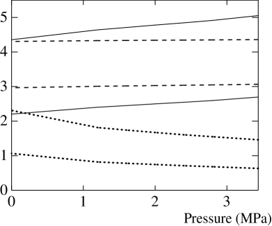
FIG. 1.: The integrals in Equations (44), (45), and (48). The solid lines give $d/g_{\rm H}\Delta^{2}\xi_{\rm GL}$, dashed $\lambda_{\rm SG}/K\Delta^{2}$ and dotted $\lambda_{\rm SHV1}\hbar/2mg_{\rm H1}\Delta^{2}\xi_{\rm GL}^{2}$. Out of similar lines, the upper ones always correspond to specular surface scattering and the lower to diffuse scattering.

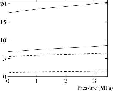
FIG. 2.: The integrals for surface-dipole terms in Equations (46) and (47). The solid lines give $b_{2}/g_{\rm D}\Delta^{2}\xi_{\rm GL}$ and the dashed $b_{4}/g_{\rm D}\Delta^{2}\xi_{\rm GL}$. For both quantities, the upper lines correspond to specular surface scattering and the lower to diffuse scattering.

All the vortex terms except $\lambda_{\rm LG}$ (18) have been calculated in Ref. [25].

All the results of this and the previous section are, of course, identical in the limit where both theories are valid: weak coupling near $T_{\rm c}$.

V Determination of parameters

In his section we analyze a few experiments in order to deduce the values of parameters $F_{0}^{\rm a}$, $F_{2}^{\rm a}$, and $g_{\rm D}$. We apply trivial strong-coupling corrections to the gap $\Delta$, as explained at the end of Section III. For the molar volume $v=mN_{\rm A}/\rho$ as a function of pressure we assume the fit in Ref. [35].

The parameter $F_{0}^{\rm a}$ can be obtained from measurements in the normal state: the specific heat and the nuclear susceptibility. For the specific heat we use the measurements by Greywall [35]. The susceptibility has been measured by Ramm et al [51] and by Hensley et al [52] with essentially identical results. Unfortunately, it has been measured only below 2.9 MPa, and depending on the extrapolation alone, the relative error in $1+F_{0}^{\rm a}$ may be as large as 10% at the melting pressure. Examples are the simple fit $F_{0}^{\rm a}=-0.909+0.0055v\ {\rm cm}^{-3}$ and the nonmonotonic $F_{0}^{\rm a}(p)$ fit in Ref. [53].

The reduced nuclear susceptibility in the superfluid state, $\chi(T)/\chi_{\rm n}$ (22), has been measured by Corruccini and Osheroff [54], by Ahonen et al [55], and by Scholz et al [56, 57]. (There has been a discrepancy between the susceptibility measured by NMR and by a SQUID magnetometer [43], but that is probably caused by difficulties in calibration [58].) $\chi(T)/\chi_{\rm n}$ depends only on two parameters, $F_{0}^{\rm a}$ and $F_{2}^{\rm a}$. (We treat the trivial strong-coupling corrections as fixed, and use only the low-field limit of the Scholz data.) If we assume $F_{0}^{\rm a}$ given by Ramm and Hensley et al, only $F_{2}^{\rm a}$ remains to be fitted. We find that a nonzero pressure-independent value of $F_{2}^{\rm a}$ does not improve the fit essentially compared to $F_{2}^{\rm a}\equiv 0$. Since we believe that $F_{2}^{\rm a}$ cannot have strong pressure dependence, the simple choice $F_{2}^{\rm a}\equiv 0$ seems most attractive to us. Scholz finds $F_{2}^{\rm a}\approx-1$ with a weak-coupling fit [57], but this tendency is largely removed by the inclusion of trivial strong-coupling corrections. Note that the susceptibility data could be equally consistent with $F_{2}^{\rm a}\equiv-0.7$, say, but that would imply a systematic reduction of $F_{0}^{\rm a}$ by -0.025 from the results by Ramm and Hensley et al. Therefore we take $F_{2}^{\rm a}\equiv 0$ in the following. For $F_{0}^{\rm a}$ we use the simple fit given above because it is in better agreement with the reduced susceptibility at the melting pressure [54] than the fit by Halperin and Varoquaux. Note that at zero pressure our choice is not far off from the relation between $F_{0}^{\rm a}$ and $F_{2}^{\rm a}$ based on the ”catastrophic relaxation” by Bunkov et al [59]. There exists also other attempts to get $F_{2}^{\rm a}$ [60, 61, 62].

The dipole constant $g_{\rm D}$ has to be extracted from experiments because its value cannot be calculated accurately in the quasiclassical theory (Sect. III). The most straightforward way to get $g_{\rm D}$ is to measure the B phase longitudinal NMR frequency $\Omega_{\parallel}$. A direct measurement of $\Omega_{\parallel}$ has been made by Bloyet et al [63] and Candela et al [61]. These experiments were done at low temperatures in the collisionless regime. According to the collisionless theory in a small magnetic field [64]

$$\Omega_{\parallel}^{2}={45\Delta^{2}g_{\rm D}\over\hbar^{2}N(0)}\left({1\over\lambda}+{2\over 3}F_{0}^{\rm a}+{1\over 15}F_{2}^{\rm a}\right)$$ (49)

where the function $\lambda(T)$ is defined in the Appendix. An alternative is to extract $\Omega_{\parallel}$ from transverse NMR frequency in surface-oriented texture. These measurements have been done by Osheroff et al. [65], by Ahonen, Krusius, and Paalanen [55] (results tabulated in Ref. [66]), by Spencer, Alexander and Ihas [67], and by Hakonen et al. [68]. Because the external magnetic field in these experiments reduces the frequency difference between normal and superfluid precession, these experiments have to be analyzed using hydrodynamic theory. There $\Omega_{\parallel}$ is related to $g_{\rm D}$ via [15]

$$\Omega_{\parallel}^{2}={15\mu_{0}\gamma^{2}\Delta^{2}g_{\rm D}\over\chi}.$$ (50)

Both relations (49) and (50) imply that the temperature dependence of $\Omega_{\parallel}$ is fully determined by the energy gap $\Delta$ and the $\lambda$ function (56) or the susceptibility $\chi$ (22).

A third way to get $g_{\rm D}$ is so-called g shift of the transverse NMR frequency $\omega$ from the Larmor frequency $\omega_{0}$. According to Ref. [17]

$${\omega-\omega_{0}\over\omega_{0}}={4\mu_{0}a\over 5\chi}.$$ (51)

The g shift was measured by Osheroff [69] at the melting pressure and by Kycia et al [42] below 2.17 MPa. [We note that these measurements are done in such a high field that the expressions given in this paper are no more reliable near $T_{\rm c}$. However, Kycia et al measure the g-shift as a function of magnetization, and this plot is found field independent, both experimentally and theoretically [42]. The only consequence is that the temperature $T$ in Fig. 3 is the temperature according to the weak-field susceptibility (22), which differs from the true temperature near $T_{\rm c}$.]

We plot $g_{\rm D}$ obtained by all three methods in Fig. 3.

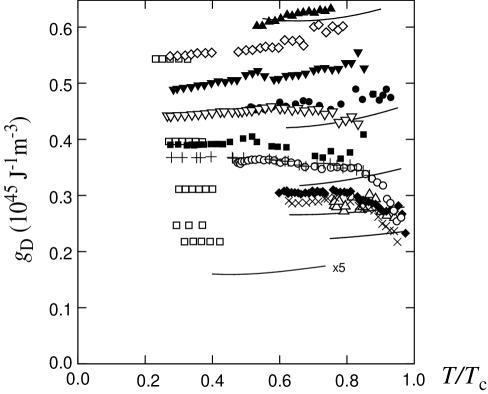
FIG. 3.: Plotted as a function of temperature, $g_{\rm D}$ interpreted from different experiments according to trivial strong-coupling model. In ideal case $g_{\rm D}$ should be independent of temperature. We have used the transverse NMR frequency measured by Osheroff et al. [65] ($\blacktriangle$ 3.44 MPa), by Ahonen, Krusius, and Paalanen [55] ($\lozenge$ 3.2 MPa, $\blacktriangledown$ 2.9 MPa, $\triangledown$ 2.54 MPa, $\blacksquare$ 2.11 MPa $+$ 1.87 MPa,), and by Hakonen et al. [68] ($\bullet$ 2.5 MPa, $\circ$ 1.55 MPa, $\blacklozenge$ 1.02 MPa, $\times$ 0.5 MPa, $\vartriangle$ 0.05 MPa). We also used the longitudinal NMR frequency measured by Candela et al. [61] ($\square$, from top to bottom 3.3, 2.1, 1.2, 0.61, and 0.03 MPa). For comparison, there are curves that are determined from the g-shift measurements by Osheroff [69] (curve with label $\times 5$, reduced by factor ${1/5}$) and by Kycia et al [42] (curves, from top to bottom 2.17, 1.3, 0.7, 0.3, and 0.11 MPa)

Let us first ignore the g-shift data (lines). It can be seen that the data for $g_{\rm D}$ at each pressure is almost independent of temperature, as required by theory. We note that in order to reach this constancy it really is necessary that the longitudinal and transverse data of $\Omega_{\parallel}$ are analyzed with collisionless and hydrodynamic theories, respectively. Equally important is that we use trivial strong-coupling corrections. The value of $g_{\rm D}$ (but not the temperature dependence) also depends on $F_{1}^{\rm s}$ and $T_{\rm c}$, for which we use the measurements by Greywall [35].

The $g_{\rm D}$ data as a function of pressure is plotted in Fig. 4. It contains all the same data as Fig. 3 and some additional data.

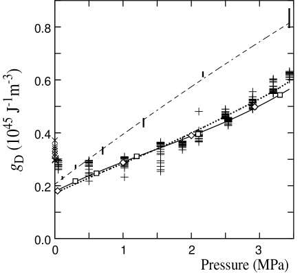
FIG. 4.: Plotted as a function of pressure, $g_{\rm D}$ interpreted from different experiments according to the trivial strong-coupling model. The data from $\Omega_{\parallel}$ in transverse NMR ($+$), from longitudinal NMR by Candela et al ($\square$), and g shift (bars) are the same as in Fig. 3. In addition there is data from zero-field longitudinal NMR measurements by Bloyet et al [63] ($\lozenge$) and transverse surface-oriented NMR measurements at saturated vapor pressure in the temperature range $T/T_{\rm c}=0.83\ldots 0.86$ by Spencer et al [67] ($\times$). The solid and dashed lines approximate the data from longitudinal NMR and g shift, receptively. The dotted line is the model of Eq. (52) with $\epsilon_{c}=0.45k_{\rm B}T_{\rm F}$. It is argued in the text that $g_{\rm D}$ given by $\Omega_{\parallel}$ is the correct one, and the difference between $g_{\rm D}$’s deduced from the g shift and $\Omega_{\parallel}$ is a measure of nontrivial strong-coupling corrections.

It can be seen that the longitudinal and transverse measurements of $\Omega_{\parallel}$ agree very well at intermediate pressures, but there is a difference at both high and low pressures. Theoretically the ratio of collisionless and hydrodynamic $\Omega_{\parallel}$ (at the same pressure) depends only on the reduced temperatures $T_{1}/T_{\rm c}$ and $T_{2}/T_{\rm c}$ of the two measurements and on $F_{0}^{\rm a}$, $F_{2}^{\rm a}$, and $\Delta C/C_{\rm n}$. The difference in the effective $g_{\rm D}$ obtained by the two methods seems at low pressures much larger than the expected uncertainties of the parameters, and remains unexplained. Both the positive slope of $g_{\rm D}(T)$ (Fig. 3) at high pressures and the difference between transverse and longitudinal data could be reduced by giving $F_{2}^{\rm a}$ a negative value ($\approx-0.7$ at high pressures), but only at the expense of impaired fit of the $\chi(T)/\chi_{\rm n}$.

We believe that the nontrivial strong coupling corrections are small in the expressions for $\Omega_{\parallel}$ (49)-(50), which are based on expectation values in an unperturbed order parameter. [There are nontrivial corrections to $\chi$ [27], but as long as (22) can reproduce (possibly with incorrect $F_{2}^{\rm a}$) the measured $\chi$, the value obtained for $g_{\rm D}$ is unaffected.] The collisionless $\Omega_{\parallel}$ data is fitted by solid line in Fig. 4. The values obtained for $g_{\rm D}$ depend on $F_{0}^{\rm a}$, $T_{\rm c}$, $N(0)$, $F_{2}^{\rm a}$, and $\Delta C/C_{\rm n}$, and must be revised if more accurate values of these become available, for example, via improved measurement of the temperature [70].

We can also estimate $g_{\rm D}$ based on the simple model of Eq. (21). Assuming $\bar{R^{2}}=1$ and making the sum at $T=T_{\rm c}$ gives

$$g_{\rm D}={\mu_{0}\over 40}\left(\hbar\gamma N(0)\ln{1.1339\epsilon_{c}\over k_{\rm B}T_{\rm c}}\right)^{2}.$$ (52)

We take the cut-off energy $\epsilon_{c}$ proportional to the Fermi temperature defined by $T_{\rm F}=3\rho/4N(0)k_{\rm B}m$. As shown by dotted line in Fig. 4, the resulting expression fits nicely the experimental data for the constant of proportionality $\epsilon_{c}/k_{\rm B}T_{\rm F}=0.45$. The agreement may be accidental, however, because there is no fundamental justification for the approximations made.

Let us next study the $g_{\rm D}$ data based on the g-shift. It is also rather independent of the temperature (lines in Fig. 3). Fig. 4 shows that the $g_{\rm D}$ data (bars) at different pressures are well consistent with each other: the low pressure data extrapolates well to the melting pressure data by Osheroff. However, $g_{\rm D}$ deduced from the g shift differs essentially from the determinations based on $\Omega_{\parallel}$, especially at high pressures. The reason for this is that the expression for $a$ (25) has substantial strong-coupling corrections that are not included in the scaling of the energy gap $\Delta$. This can be seen by comparing the $T\rightarrow T_{\rm c}$ limit of trivial strong-coupling $a$ (25), denoted by $a_{\rm TSC}$, with the Ginzburg-Landau limit $a_{\rm GL}$ (38). We find

$${a_{\rm GL}\over a_{\rm TSC}}={a_{\rm GL}\over a_{\rm WC}}={g_{\rm H}\over g_{\rm H}^{\rm WC}}{\beta_{345}^{\rm WC}\over\beta_{345}}.$$ (53)

where WC denotes weak-coupling. It is well known that $\beta_{345}$ differs substantially from its weak coupling value [46, 41, 42, 43]. This explains the difference in the apparent $g_{\rm D}$ deduced from g shift and $\Omega_{\parallel}$. The new thing in the present analysis compared to Ref. [42] is that the difference is not limited to the Ginzburg-Landau region, but because of the weak dependency of the apparent $g_{\rm D}$ on temperature (Fig. 3), it persists almost unchanged at all temperatures.

We conclude this section with a comparison of theoretical and experimental dipole velocity $v_{\rm D}$. Theoretically this quantity is related to coefficients $a$ (25) and $\lambda_{\rm HV}$ (28) by the relation $v_{\rm D}^{2}=2a/(5\lambda_{\rm HV})$. It has been measured by Nummila et al [71]. Originally they compared their result to a theory that turned out to be in error, see discussion in Refs. [29, 72]. The comparison with the present theory is given in Fig. 5. We have used trivial strong-coupling theory, parameters as described above and $g_{\rm D}$ from solid line in Fig. 4.

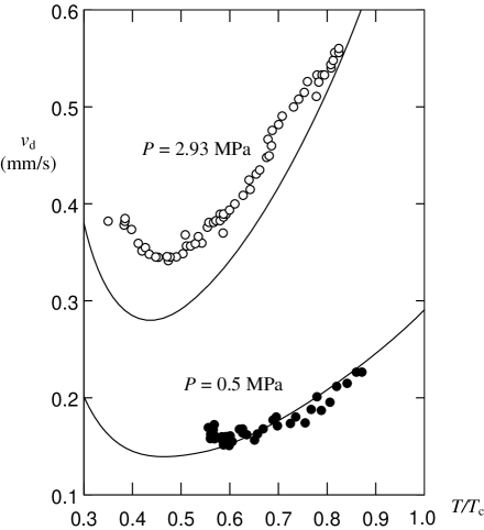
FIG. 5.: The dipolar velocity $v_{\rm D}$. The circles are experimental data from Ref. [71]. The solid lines are theory based on Equations (25) and (28), where all parameter values are fixed by other measurements as explained in the text.

Because both $a$ (38) and $\lambda_{\rm HV}$ (40) are proportional to $\beta_{345}^{-1}$ in the Ginzburg-Landau region, the uncertainty discussed in connection with $a$ is expected to cancel out in $v_{\rm D}$. There also exists a direct measurement of $\lambda_{\rm HV}$ [29]. It also shows deviation from the trivial strong-coupling model, but the differences are not of similar type as for $a$, and are presently not understood.

Above we have discussed all input parameters of the trivial-strong-coupling hydrostatic theory except $F^{\rm a}_{1}$ and $F^{\rm a}_{3}$. Out of the bulk terms only the gradient coefficients (29) and (30) depend on these. There is several independent evidence that $F^{\rm a}_{1}\approx-1$ at high pressures [73, 74, 75] but $F^{\rm a}_{3}$ is not known.

VI Conclusions

We have presented a summary of the hydrostatic theory in superfluid ³He-B. Several new analytic and numerical results were included. Some experimental data was analyzed in order to extract the parameters of the theory. A particular goal was to understand how well the B phase is described by the trivial strong-coupling model. We found that some quantities ($\chi$, $g_{\rm D}$, $v_{\rm D}$) can successfully be calculated, but there are other quantities ($a$, $\lambda_{\rm HV}$) that may be wrong by 50% in this model. The parameter $g_{\rm D}$ has direct relevance also for the A phase, where it has been used in comparison between theory and experiment (see Ref. [76], for example).

The first application of the results calculated here has been the comparison of the ratio $d/a$ [from equations (44) and (38)] to experiments in Ref. [77]. More recently, Kopu et al [78] applied the hydrostatic theory to a rotating cylindrical container. They calculated the NMR line shape and studied the optimal conditions for observing single vortex lines. Another application is the Josephson $\pi$ state observed recently [3]. This effect was found to depend crucially on the texture at the Josephson junction [79, 33]. The texture is also essential in several experiments of superfluid ³He in aerogel. For example, the identification of the B phase was based on its texture-dependent NMR spectrum [80]. For the present, the textural parameters in aerogel have been evaluated only in the Ginzburg-Landau region in the homogeneous scattering model [81]. These developments demonstrate that there still are open problems in superfluid ³He and in many cases a proper understanding of the hydrostatic theory is a prerequisite for solving them.

Appendix

We give here some equations that complete the theory presented above. The weak-coupling energy gap $\Delta(T)$ is determined by the equation

$$\ln{T\over T_{\rm c}}+\pi T\sum_{n=-\infty}^{\infty}\left[{1\over|\epsilon_{n}|}-{1\over\sqrt{\epsilon_{n}^{2}+\Delta^{2}}}\right]=0,$$ (54)

where the Matsubara energies $\epsilon_{n}=\pi T(2n-1)$ with $n=0,\pm 1,...\pm\infty$. The $Z_{j}(T)$ functions are defined by

$$Z_{j}=\pi k_{\rm B}T\Delta^{j-1}\sum_{n=-\infty}^{\infty}(\epsilon_{n}^{2}+\Delta^{2})^{-j/2},$$ (55)

$Y(T)=1-Z_{3}(T)$. The $\lambda(T)$ function [64], which equals to $1-f(T)$ defined in Ref. [82], can be written as

$$\lambda=\pi k_{\rm B}T\sum_{n=-\infty}^{\infty}{\Delta\over\sqrt{\epsilon_{n}^{2}+\Delta^{2}}(\sqrt{\epsilon_{n}^{2}+\Delta^{2}}+\Delta)}.$$ (56)

The numerical calculation of the functions is discussed in Ref. [83].

The gradient energies (10) and (13) can be written in different forms using the identities [17]

$$\partial_{i}R_{\alpha j}\partial_{i}R_{\alpha j} = 4(1-\cos\theta)(\partial_{i}\hat{n}_{j})^{2}=4(1-\cos\theta)\{(\nabla\times\hat{\bf n})^{2}+(\nabla\cdot\hat{\bf n})^{2}+\nabla\cdot[(\hat{\bf n}\cdot\nabla)\hat{\bf n}-\hat{\bf n}(\nabla\cdot\hat{\bf n})]\}$$ (57)

$$\partial_{i}R_{\alpha i}\partial_{j}R_{\alpha j} = (1-\cos\theta)[2(\nabla\times\hat{\bf n})^{2}+(1-\cos\theta)(\nabla\cdot\hat{\bf n})^{2}-(1-\cos\theta)(\hat{\bf n}\cdot\nabla\times\hat{\bf n})^{2}-2\sin\theta(\nabla\cdot\hat{\bf n})(\hat{\bf n}\cdot\nabla\times\hat{\bf n})]$$ (58)

$$\partial_{i}R_{\alpha j}\partial_{j}R_{\alpha i} = (1-\cos\theta)\{2(\nabla\times\hat{\bf n})^{2}+(1-\cos\theta)(\nabla\cdot\hat{\bf n})^{2}-(1-\cos\theta)(\hat{\bf n}\cdot\nabla\times\hat{\bf n})^{2}$$ (60)

$$-2\sin\theta(\nabla\cdot\hat{\bf n})(\hat{\bf n}\cdot\nabla\times\hat{\bf n})+2\nabla\cdot[(\hat{\bf n}\cdot\nabla)\hat{\bf n}-\hat{\bf n}(\nabla\cdot\hat{\bf n})]\}$$

$$\hat{s}_{i}R_{\alpha i}\partial_{j}R_{\alpha j} = -(1-\cos\theta)\hat{\bf s}\cdot[(\hat{\bf n}\cdot\nabla)\hat{\bf n}-\hat{\bf n}(\nabla\cdot\hat{\bf n})]\}.$$ (61)

Using these it can be seen that $F_{\rm G}$ (10) has a pure divergence term $\propto\nabla\cdot[(\hat{\bf n}\cdot\nabla)\hat{\bf n}-\hat{\bf n}(\nabla\cdot\hat{\bf n})]$. The prefactor of this term is half of the value of that by Smith, Brinkman and Engelsberg [17]. With present definitions the other half is transferred to the surface term (13).

REFERENCES

- [1] O.V. Lounasmaa and E.V. Thuneberg, Proc. Natl. Acad. Sci. USA 96, 7760 (1999).
- [2] A. Golov, J.V. Porto, D.A. Geller, N. Mulders, G.J. Lawes, and J.M. Parpia, Physica B 280, 134 (2000).
- [3] A. Marchenkov, R.W. Simmonds, S. Backhaus, A. Loshak, J.C. Davis, and R.E. Packard, Phys. Rev. Lett. 83, 3860 (1999).
- [4] L.D. Landau and E.M. Lifshitz, Fluid Mechanics (Pergamon Press, Oxford, 1987).
- [5] A.J. Leggett, Rev. Mod. Phys. 47, 331 (1975).
- [6] W.F. Brinkman and M.C. Cross, in Progress in Low Temperature Physics, Vol VIIA, ed. D.F. Brewer (North Holland, 1978), p. 105.
- [7] J.W. Serene and D. Rainer, Phys. Rep. 101, 221 (1983).
- [8] A.L. Fetter, in Progress in Low Temperature Physics, Vol. X, ed. D.F. Brewer (Elsevier, 1986), p. 1.
- [9] M.M. Salomaa and G.E. Volovik, Rev. Mod. Phys. 59, 533 (1987), 60, 573 (1988).
- [10] G.A. Kharadze, in Helium Three, ed. W.P. Halperin and L.P. Pitaevskii (Elsevier, Amsterdam 1990), p. 167.
- [11] D. Vollhardt and P. Wölfle, The superfluid phases of helium 3 (Taylor & Francis, London 1990).
- [12] J. Bardeen, L.N. Cooper, and J.R. Schrieffer, Phys. Rev. 108, 1175 (1957).
- [13] J.C. Wheatley, Rev. Mod. Phys. 47, 415 (1975).
- [14] G.W. Swift, J.P. Eisenstein, and R.E. Packard, Phys. Rev. Lett. 45, 1955 (1980).
- [15] A.J. Leggett, Ann. Phys. (New York) 85, 11 (1974).
- [16] S. Engelsberg, W.F. Brinkman, and P.W. Anderson, Phys. Rev. A 9, 2592 (1974).
- [17] H. Smith, W.F. Brinkman, and S. Engelsberg, Phys. Rev. B15, 199 (1977).
- [18] W.F. Brinkman, H. Smith, D.D. Osheroff, and E.I. Blount, Phys. Rev. Lett 33, 624 (1974).
- [19] G.E. Volovik and V.P. Mineev, Zh. Eksp. Teor. Fiz. 86, 1667 (1984) [Sov. Phys. JETP 59, 972 (1984)].
- [20] E.V. Thuneberg, Phys. Rev. B 33, 5124 (1986).
- [21] I.A. Fomin and M. Vuorio, J. Low Temp. Phys. 21, 271 (1975).
- [22] W. Zhang, J. Kurkijärvi, and E.V. Thuneberg, Phys. Rev. B36, 1987 (1987).
- [23] A.D. Gongadze, G.E. Gurgenishvili, and G.A. Kharadze, Fiz. Nizk. Temp. 7, 821 (1981) [Sov. J. Low Temp. Phys. 7, 397 (1981)].
- [24] P.J. Hakonen, M. Krusius, M.M. Salomaa, J.T. Simola, Yu.M. Bunkov, V.P. Mineev, and G.E. Volovik, Phys. Rev. Lett. 51, 1362 (1983).
- [25] E.V. Thuneberg, Phys. Rev. B 36, 3583 (1987).
- [26] J.W. Serene and D. Rainer, Phys. Rev. B 17, 2901 (1978).
- [27] J.W. Serene and D. Rainer, in Quantum fluids and solids, eds. S.B. Trickey, E.D. Adams, and J.W. Dufty (Plenum, New York, 1977), p. 111.
- [28] R.S. Fishman and J.A. Sauls, Phys. Rev. B 33, 6068 (1986).
- [29] J.S. Korhonen, Yu.M. Bunkov, V.V. Dmitriev, Y. Kondo, M. Krusius, Yu.M. Mukharskiy, Ü. Parts, and E.V. Thuneberg, Phys. Rev. B 46, 13983 (1992).
- [30] V.P. Mineev, Zh. Eksp. Teor. Fiz. 90, 1236 (1986) [Sov. Phys. JETP 63, 721 (1986)].
- [31] M. Dörfle, Phys. Rev. B 23, 3267 (1981); note incorrect powers of 2 in equations (5.3) and (5.4).
- [32] L.J. Buchholtz, Phys. Rev. B 33, 1579 (1986).
- [33] J. Viljas and E.V. Thuneberg, to be published.
- [34] M. Fogelström and J. Kurkijärvi, J. Low Temp. Phys. 98, 195 (1995); erratum 100, 597 (1995).
- [35] D.S. Greywall, Phys. Rev. B 33, 7520 (1986).
- [36] V.L. Ginzburg and L.D. Landau, Zh. Eksp. Teor. Fiz. 20, 1064 (1950).
- [37] N.D. Mermin and C. Stare, Phys. Rev. Lett. 30, 1135 (1973).
- [38] V. Ambegaokar, P.G. deGennes, and D. Rainer, Phys. Rev. A 9, 2676 (1974), 12, 345 (1975).
- [39] V. Ambegaokar and N.D. Mermin, Phys. Rev. Lett. 30, 81 (1973).
- [40] A.L. Fetter, in Quantum Statistics and the Many-Body Problem, eds. S.B. Trickey, W.P. Kirk, and J.W. Dufty (Plenum, New York, 1975), p. 127.
- [41] Y.H. Tang, I. Hahn, H.M. Bozler, and C.M. Gould, Phys. Rev. Lett. 67, 1775 (1991).
- [42] J.B. Kycia, T.M. Haard, M.R. Rand, H.H. Hensley, G.F. Moores, Y. Lee, P.J. Hamot, D.T. Sprague, W.P. Halperin, and E.V. Thuneberg, Phys. Rev. Lett. 72, 864 (1994).
- [43] I. Hahn, S.T.P. Boyd, H.M. Bozler, and C.M. Gould, Phys. Rev. Lett. 81, 618 (1998).
- [44] D. Rainer and J.W. Serene, Phys. Rev. B 13, 4745 (1976).
- [45] D. Rainer and J.W. Serene, J. Low Temp. Phys. 38, 601 (1980).
- [46] J.A. Sauls and J.W. Serene, Phys. Rev. B 24, 183 (1981).
- [47] K. Bedell, Phys. Rev. B 26, 3747 (1982).
- [48] K. Levin and O.T. Valls, Phys. Rep. 98, 1 (1983).
- [49] D.C. Sagan, P.G.N. deVegvar, E. Polturak, L. Friedman, S.-S. Yan, E.L. Ziercher and D.M. Lee, Phys. Rev. Lett. 53, 1939 (1984).
- [50] U.E. Israelsson, B.C. Crooker, H.M. Bozler and C.M. Gould, Phys. Rev. Lett. 53, 1943 (1984).
- [51] H. Ramm, P. Pedroni, J.R. Thompson, and H. Meyer, J. Low Temp. Phys. 2, 539 (1970).
- [52] H.H. Hensley, Y. Lee, P. Hamot, T. Mizusaki, and W.P. Halperin, J. Low Temp. Phys. 90, 149 (1993).
- [53] W.P. Halperin and E. Varoquaux, in Helium Three, ed. W.P. Halperin and L.P. Pitaevskii (Elsevier, Amsterdam 1990), p. 353.
- [54] L.R. Corruccini and D.D. Osheroff, Phys. Rev. B 17, 126 (1978).
- [55] A.I. Ahonen, M. Krusius, and M.A. Paalanen, J. Low Temp. Phys. 25, 421 (1976).
- [56] R.F. Hoyt, H.N. Scholz, and D.O. Edwards, Physica B 107, 287 (1981).
- [57] H.N. Scholz, Thesis (Ohio State University, 1981).
- [58] C.M. Gould, private communication.
- [59] Yu.M. Bunkov, S.N. Fisher, A.M. Guénault, C.J. Kennedy, and G.R. Pickett, J. Low Temp. Phys. 89, 27 (1992).
- [60] R.S. Fishman and J.A. Sauls, Phys. Rev. B 38, 2526 (1988).
- [61] D. Candela, D.O. Edwards, A. Heff, N. Masuhara, Y. Oda, and D.S. Sherrill, Phys. Rev. Lett. 61, 420 (1988).
- [62] R. Movshovich, N. Kim, and D.M. Lee, Phys. Rev. Lett. 64, 431 (1990).
- [63] D. Bloyet, E. Varoquaux, C. Vibet, O. Avenel, P.M. Berglund, and R. Combescot, Phys. Rev. Lett. 42, 1158 (1979); C. Vibet, thesis, L’Université Paris-Sud, Centre d’Orsay, 1979 (unpublished).
- [64] R.S. Fishman, Phys. Rev. B 36, 79 (1987).
- [65] D.D. Osheroff, S. Engelsberg, W.F. Brinkman, and L.R. Corruccini, Phys. Rev. Lett. 34, 190 (1975).
- [66] J.C. Wheatley, in Progress in Low Temperature Physics, Volume VIIA, ed. D.F. Brewer (North-Holland, 1978), p. 1.
- [67] G.F. Spencer, P.W. Alexander, and G.G. Ihas, Physica B 107, 289 (1981).
- [68] P.J. Hakonen, M. Krusius, M.M. Salomaa, R.H. Salmelin, J.T. Simola, A.D. Gongadze, G.E. Vachnadze, and G.A. Kharadze, J. Low Temp. Phys. 76, 225 (1989).
- [69] D.D. Osheroff, unpublished, g-shift for in the range 0.39-0.74 at the melting pressure.
- [70] R.J. Solen Jr. and W.E. Fogle, Physics Today 50, no. 8 Part 1, 36 (1997).
- [71] K.K. Nummila, P.J. Hakonen, and O.V. Magradze, Europhys. Lett. 9, 355 (1989).
- [72] A. Gongadze, G. Kharadze, and G. Vachnadze, Fiz. Nizk. Temp. 23, 546 (1997) [Low Temp. Phys. 23, 405 (1997)].
- [73] D.D. Osheroff, W. van Roosbroeck, H. Smith, and W.F. Brinkman, Phys. Rev. Lett. 38, 134 (1977).
- [74] D.S. Greywall, Phys. Rev. B 27, 2747 (1983).
- [75] Ü. Parts, V.M.H. Ruutu, J.H. Koivuniemi, M. Krusius, E.V. Thuneberg, and G.E. Volovik, Physica B 210, 311 (1995).
- [76] J.M. Karimäki and E.V. Thuneberg, Phys. Rev. B 60, 15290 (1999).
- [77] J.S. Korhonen, A.D. Gongadze, Z. Janú, Y. Kondo, M. Krusius, Yu.M. Mukharsky, and E.V. Thuneberg, Phys. Rev. Lett. 65, 1211 (1990).
- [78] J. Kopu, R. Schanen, R. Blaauwgeers, V.B. Eltsov, M. Krusius, J.J. Ruohio, and E.V. Thuneberg, J. Low Temp. Phys. 120, 213 (2000).
- [79] J.K. Viljas and E.V. Thuneberg, Phys. Rev. Lett. 83, 3868 (1999).
- [80] H. Alles, J.J. Kaplinsky, P.S. Wootton, J.D. Reppy, J.H. Naish, and J.R. Hook, Phys. Rev. Lett. 83, 1367 (1999).
- [81] E.V. Thuneberg, in Quasiclassical Methods in Superconductivity and Superfluidity, Verditz 96, ed. D. Rainer and J.A. Sauls (1998) p. 53; cond-mat/9802044.
- [82] A.J. Leggett and S. Takagi, Ann. Phys. (New York) 106, 79 (1977).
- [83] http://boojum.hut.fi/research/theory/qc/bcsgap.html