[

Stochastic Ballistic Annihilation and Coalescence

Abstract

We study a class of stochastic ballistic annihilation and coalescence models with a binary velocity distribution in one dimension. We obtain an exact solution for the density which reveals a universal phase diagram for the asymptotic density decay. By universal we mean that all models in the class are described by a single phase diagram spanned by two reduced parameters. The phase diagram reveals four regimes, two of which contain the previously studied cases of ballistic annihilation. The two new phases are a direct consequence of the stochasticity. The solution is obtained through a matrix product approach and builds on properties of a $q$-deformed harmonic oscillator algebra.

]

Systems of reacting particles are used to model a whole gamut of phenomena relevant to fields ranging from chemical physics through statistical physics to mathematical biology. In some applications the particles represent chemical or biological species [1, 2]; in other cases they are to be interpreted as composite objects such as aggregating traffic jams [3]. Excitations can also be treated as interacting particles, one example being laser-induced excitons in certain crystals [4]. Furthermore, domain walls occurring in a number of different contexts such as growth and coarsening processes [5, 6] have dynamics with a natural particle interpretation.

Generally these systems are defined through nonequilibrium dynamics. Given such a wide variety of nonequilibrium reaction systems, it is natural to ask if they can be divided into distinct groups akin to the universality classes known for equilibrium systems.

Two reactions that have been extensively studied are single species annihilation ($A{+}A{\to}\emptyset$) and coalescence ($A{+}A{\to}A$). A particularly striking result is that if the reactant motion is diffusive, the two processes belong to the same universality class [7] and the density decay is independent of the reaction rate in two dimensions and below. Moreover, these diffusive systems have also served as prototypes for the development of a variety of theoretical tools ranging from field theoretic renormalization group (RG) [8], to exact methods in low dimensions [9].

On the other hand, much less is known about the same reactions when the motion is ballistic (deterministic) despite the relevance of such motion to the modeling of growth and coarsening processes [5, 6]. A seminal model was introduced and solved by Elskens and Frisch [10] and describes pairwise annihilation of oppositely moving particles in one dimension (1D). That study was restricted to particles that react upon contact with probability one. More recently some results have been obtained for systems in which the reaction probability is less than one, thus introducing stochasticity into the evolution [11, 12].

In this work we introduce a class of 1D stochastic ballistic reaction systems. The class includes both ballistic annihilation and coalescence and incorporates as special limits the models of [10] and [12]. We obtain an exact solution for the density decay which reveals a single phase diagram common to all combinations of ballistic annihilation and coalescence. This demonstrates a universality of the two processes. The universality is stronger than that usually discussed in an RG context and can be likened to a law of corresponding states. The phase diagram generically comprises four decay regimes in contrast to the two previously known [10]. The new phases are a result of the stochasticity of the reactions.

Our exact solution is based on the invariance of certain properties of our class of models under change of the initial spacing of the particles. As a consequence the long time density may be determined exactly through a matrix product approach of the type introduced in [13]. We use this property, and employ recent results on $q$-deformed algebras [14], to analyse the asymptotic density decay.

We now define the class of models to be considered. At time $t=0$ reactants are placed on a line with nearest-neighbor distances chosen independently from a continuous exponential distribution. The unit of length is chosen so that the initial density is $\varrho=1$. Although we consider here a Poisson initial condition, our methods are extendible to more general initial distributions (see below). Each particle is assigned a velocity $+c$ (right-moving) or $-c$ (left-moving) with probability $f_{R}$ and $f_{L}=1-f_{R}$ respectively. Particles move ballistically until two collide, at which point one of four outcomes follows, see Fig. 1: the particles pass through each other with probability $q$; the particles coalesce into a left (right) moving particle with probability $p\eta_{L}$ ($p\eta_{R}$); the particles annihilate with probability $p(1-\eta_{L}-\eta_{R})$. Here $p=1-q$ is the probability that some reaction occurs.

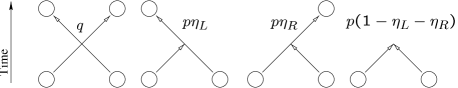
FIG. 1.: The possible reactions and their probabilities.

Before describing our method of solution, we present our main results summarized in the phase diagram Fig. 2. Two important quantities that emerge are the reduced densities $f_{L}^{\ast}=f_{L}(1-\eta_{R})$ and $f_{R}^{\ast}=f_{R}(1-\eta_{L})$. The phase diagram is spanned by $q$, the probability of not reacting, and $\chi=f_{R}^{\ast}/f_{L}^{\ast}$, the ratio of reduced densities. For simplicity we consider $\chi\leq 1$ which results in eventual extinction of right-moving particles; $\chi=1$ is a special case where both species die out. The case $\chi>1$ can be treated using the symmetry of the model under left-right interchange $f_{R}\leftrightarrow f_{L}$ and $\eta_{R}\leftrightarrow\eta_{L}$ i.e. $\chi\to 1/\chi$.

FIG. 2.: The phase diagram of the model for $\chi\leq 1$. The behavior for $\chi>1$ can be deduced from that with $\chi<1$ via a left-right symmetry (see text).

The different phases—of which two are regions and two are lines in the phase diagram—correspond to four qualitative long-time density decays. When $\chi<q^{2}$ the decay is purely exponential of the form $\varrho\simeq\varrho_{\infty}+b_{1}\exp(-\alpha_{1}t)$; when $\chi=q^{2}$ the decay is exponential, multiplied by a $t^{-1/2}$ power law $\varrho\simeq\varrho_{\infty}+b_{2}\exp(-\alpha_{2}t)/t^{1/2}$; when $q^{2}{<}\chi{<}1$ the decay exponential, multiplied by a $t^{-3/2}$ power law $\varrho\simeq\varrho_{\infty}+b_{3}\exp(-\alpha_{3}t)/t^{3/2}$; finally when $\chi=1$ the decay is pure power law $\varrho\simeq b_{2}/t^{1/2}$. The exact expressions for the coefficients $\alpha,b$ and final density $\varrho_{\infty}$ are as given in Table I. Some intriguing features that emerge from the phase diagram Figure 2 are:

(i) There is universality of ballistic annihilation and coalescence. This is manifested by the fact that all the information concerning the reactions of a particular model, along with the initial densities, are encoded into a single parameter $\chi$. For a generic choice of $\eta_{R}$, $\eta_{L}$ defining a particular annihilation-coalescence model, the same four decay regimes are found by varying the initial densities or stochasticity parameter $q$. In this way the universality can be considered as a law of corresponding states.

(ii) Two new density decays appear which were not anticipated in previous works. The first is the line $\chi=q^{2}$ and the second the region $\chi<q^{2}$. Thus for a generic value of the reaction probability $1-q$, varying the initial densities gives rise to four types of asymptotic decay.

(iii) The deterministic case $q=0$ is non-generic since along this line only two of the possible phases are traversed. For the pure annihilation model ($\eta_{R}=\eta_{L}=0$) these phases were found in [10]. Thus we refer to the entire region $q^{2}{}<{}\chi{}<1$ as the Elskens-Frisch phase.

(iv) The line $\chi=1$ (equal reduced densities) is non-generic since a single, power law, decay regime is found. The decay does not depend on the stochasticity $q$. For $\eta_{R}=\eta_{L}=0$ this special line corresponds to equal initial densities [12]. Our results show that such a special line exists for all combinations of annihilation and coalescence. This phase can be understood through the picture of [10]. Density fluctuations in the initial conditions lead to trains of left- and right-moving particles: in a length $\sim t$ the excess particle number is $\sim t^{1/2}$ which yields the $t^{-1/2}$ density decay. At long times, the train size is large and so a particle in one train encounters many particles in the other and will eventually react making the parameter $q$ irrelevant.

(v) In the two new phases ($\chi\leq q^{2}$) the two species decay at unequal rates leaving a non-zero population of left-moving particles. This is to be contrasted to the Elskens-Frisch phase ($\chi>q^{2}$) where the final density of one species is non-zero but both species decay at the same rate. A simple example of non-equal decays is the case $\eta_{R}=0,\eta_{L}=1$ ($\chi=0$). Then left-moving particles do not decay but simply absorb the right-moving particles with probability $1-q$ giving $\varrho=f_{R}{\rm e}^{-2(1-q)f_{L}ct}$. Our results show that, in general, increasing $q$ leads to a non-trivial transition at $\chi=q^{2}$ to a regime where the two species have different decay forms.

	$\varrho(t)-\varrho_{\infty}$
$\chi<q^{2}$	$\displaystyle f_{R}\left(1-\frac{f_{R}^{\ast}}{q^{2}f_{L}^{\ast}}\right){\rm e}^{-2\,\left(1-q\right)\left(f_{L}^{\ast}-f_{R}^{\ast}/q\right)ct}$
$\chi=q^{2}$	$\displaystyle\frac{f_{R}}{\sqrt{2\pi}}\left(\frac{1}{f_{L}^{\ast}f_{R}^{\ast}}\right)^{\!\frac{1}{4}}\frac{{\rm e}^{-2(\sqrt{f_{L}^{\ast}}-\sqrt{f_{R}^{\ast}})^{2}ct}}{(ct)^{1/2}}$
$q^{2}{<}\chi{<}1$	$\displaystyle\frac{K}{4\sqrt{2\pi}}\left(\frac{1}{f_{L}^{\ast}f_{R}^{\ast}}\right)^{\!\frac{3}{4}}\frac{f_{L}f_{R}^{\ast}+f_{R}f_{L}^{\ast}}{(\sqrt{f_{L}^{\ast}}-\sqrt{f_{R}^{\ast}})^{2}}\frac{{\rm e}^{-2(\sqrt{f_{L}^{\ast}}-\sqrt{f_{R}^{\ast}})^{2}ct}}{(ct)^{3/2}}$
$\chi=1$	$\displaystyle\frac{1}{\sqrt{2\pi}}\left(\frac{1}{f_{L}^{\ast}f_{R}^{\ast}}\right)^{\!\frac{1}{4}}\left(\frac{1}{ct}\right)^{\!\frac{1}{2}}$

TABLE I.: Long time density decays to the asymptotic value $\varrho_{\infty}=f_{L}(1-\chi)$. Results for $\chi>1$ can be obtained via the right-left symmetry (see text). $K$ is given by (10).

We now turn to the method of derivation of the phase diagram. The density is given by

$$\varrho(t)=f_{R}P_{S}^{(R)}(t)+f_{L}P_{S}^{(L)}(t)$$ (1)

where $P_{S}^{(L)}(t)$ and $P_{S}^{(R)}(t)$ are the probabilities that a left- and right-moving particle survive up to a time $t$ respectively. These two probabilities are related by the left-right symmetry noted previously; therefore, if we calculate $P_{S}^{(R)}(t)$ for all $\chi$ we can infer $P_{S}^{(L)}(t)$.

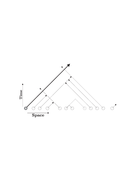
FIG. 3.: A configuration and set of trajectories and reactions for a test particle (shaded and bold line) encountering a string of $N=10$ particles. Note how changing the spacing between, for example, the fifth and sixth particles (indicated by dotted lines) alters the time sequence of the reactions but not the final survival probability.

To calculate $P_{S}^{(R)}(t)$ consider the leftmost, right-moving particle in Fig. 3 which we refer to as a test particle. From the figure one can see that the initial spacing of the particles on the line does not affect the sequence of possible reactions for any given particle, in particular for the test particle (we return to this point later). Also note that after a given time $t$, the test particle may only have interacted with the $N$ particles initially placed within a distance $X=2ct$ (and to the right) of the chosen particle. These two facts imply that the survival probability can be expressed in terms of two independent functions. The first is $F(N)$, the probability that the test particle survives reactions with the $N$ particles initially to its right, and depends only on the sequence of the $N$ particles. The second is $G(N;X)$, the probability that initially there were exactly $N$ particles in a region of size $X=2ct$. Explicitly,

$$P_{S}^{(R)}(X)=\sum_{N=0}^{\infty}F(N)G(N;X)\;.$$ (2)

Thus the problem is reduced to two separate combinatorial problems of calculating $G(N;X)$ and $F(N)$. For the Poisson initial conditions $G(N;X)=X^{N}\mbox{e}^{-X}/N!$ [15]. In the following we show how the second problem may be solved by employing a matrix product approach [13].

As an example consider a test particle encountering the string of reactants depicted in Fig. 3. We claim that the probability of the test particle surviving through this string may be written as

$$\langle W|RRRLRLLLLR|V\rangle$$ (3)

where $R,L$ are matrices (or operators) and $\langle W|$, $|V\rangle$ vectors with scalar product $\langle W|V\rangle=1$. Thus we write, in order, a matrix $R$ ($L$) for each right (left) moving particle in the initial string.

We now show that the conditions for an expression such as (3) to hold for an arbitrary string are

$$RL = qLR+p(\eta_{L}L+\eta_{R}R+[1-\eta_{L}-\eta_{R}])$$ (4)

$$\langle W|L = \langle W|(q+p\eta_{R})\qquad R|V\rangle=|V\rangle\;.$$ (5)

To understand condition (4), recall that after an interaction between a right-moving and left-moving particle there are four possible outcomes (see Fig. 1) corresponding to the four terms on the right hand side of Eq. 4 with probabilities given by the respective coefficients. Using (4), any initial matrix product such as (3) can be reduced to a sum of terms of form $\langle W|L^{s}R^{t}|V\rangle$ corresponding to all possible final states ensuing from the initial string and with coefficients equal to the probabilities of each final state. The test particle will survive such a final state and pass through the $s$ left-moving particles with probability $(q+p\eta_{R})^{s}$. The conditions (5) ensure that this probability is obtained for each possible final state.

The above approach relies on an important property of the system which is invariance of a reaction sequence with respect to changes of initial particle spacings. To understand this, consider again Fig. 3. By altering the initial spacings of the particles, the absolute times at which trajectories intersect and reactions may occur (if the reactants have survived) may be altered. For example, by increasing the spacing between the fifth and sixth particles, the trajectories of the third and fourth particles can be made to intersect first. However as we have already seen, for any particle, the order of intersections it encounters does not change and so the final states and probabilities are invariant. This invariance is manifested in the matrix product by the fact that the order in which we use the reduction rule (4) is unimportant i.e. matrix multiplication is associative.

Averaging over all initial strings of length $N$ yields

$$F(N)=\langle W|(f_{L}L+f_{R}R)^{N}|V\rangle\;.$$ (6)

To evaluate $F(N)$ we write $R=\sqrt{f_{R}^{\ast}f_{L}^{\ast}}/f_{R}\,a+\eta_{L}$ and $L=\sqrt{f_{R}^{\ast}f_{L}^{\ast}}/f_{L}\,a^{\dagger}+\eta_{R}$. One can check from (4,5) that $a,a^{\dagger}$ satisfy a $q$-deformed harmonic oscillator algebra

$$aa^{\dagger}-qa^{\dagger}a=1-q$$ (7)

$$\langle W|a^{\dagger}=\langle W|q/\sqrt{\chi}\qquad a|V\rangle=\sqrt{\chi}\,|V\rangle\;.$$ (8)

As is evident from (8) the vectors $|W\rangle$, $|V\rangle$ are eigenvectors of $a$, and are called $q$-deformed coherent states. The explicit form of these eigenvectors is known [14]. Using the above definitions (6) becomes

$$F(N)=\langle W|\left[\sqrt{f_{R}^{\ast}f_{L}^{\ast}}\,(a+a^{\dagger})+1{-}f_{L}^{\ast}{-}f_{R}^{\ast}\right]^{N}|V\rangle.$$ (9)

In the deterministic limit, $q=0$, (7) becomes $aa^{\dagger}=1$ and $a$, $a^{\dagger}$ are ladder operators. For $\chi=1$, as in [10], one can see using (8) that the matrix product (9) is equivalent to a problem of counting 1D random walks that do not return to the origin [5]. For general $q$, the evaluation of (9) poses a $q$-combinatoric problem, the solution of which we now outline.

We take advantage of recent techniques and results [14] for the calculation of matrix products such as (9). The approach is based on the fact that the eigenstates of the operator $x=a+a^{\dagger}$ (analogous to the position operator in the usual harmonic oscillator) can be expressed in terms of $q$-deformed Hermite polynomials, whose orthogonality properties and generating functions are known. Decomposing $\langle W|$ and $|V\rangle$ onto the eigenbasis of $x$ allows an integral representation of $F(N)$. From this expression the large $N$ behavior can be extracted by using standard asymptotic analysis detailed in [14]. The results are summarized in Table II in which

$$K=\prod_{n=1}^{\infty}\frac{(1-q^{n})^{4}}{(1-q^{n}\,\sqrt{\chi})^{2}(1-q^{n}/\sqrt{\chi})^{2}}\;.$$ (10)

	$A$	$B$	$\gamma$
$\chi<q^{2}$	$\displaystyle 1-\frac{1}{q^{2}}\,\frac{f_{R}^{\ast}}{f_{L}^{\ast}}$	$\left(1-q\right)\left(f_{L}^{\ast}-\frac{f_{R}^{\ast}}{q}\right)$	$\displaystyle 0$
$\chi=q^{2}$	$\displaystyle\frac{1}{\sqrt{\pi}}\left(\frac{1}{f_{L}^{\ast}f_{R}^{\ast}}\right)^{\!\frac{1}{4}}$	$\left(\sqrt{f_{L}^{\ast}}-\sqrt{f_{R}^{\ast}}\right)^{\!2}$	$\displaystyle\frac{1}{2}$
$q^{2}{<}\chi{<}1$	$\displaystyle\frac{1}{\sqrt{4\pi}}\frac{K}{(1-\sqrt{\chi})^{2}}\left(\frac{1}{f_{L}^{\ast}f_{R}^{\ast}}\right)^{\!\frac{3}{4}}$	$\left(\sqrt{f_{L}^{\ast}}-\sqrt{f_{R}^{\ast}}\right)^{\!2}$	$\displaystyle\frac{3}{2}$
$\chi=1$	$\displaystyle\frac{1}{\sqrt{\pi}}\left(\frac{1}{f_{L}^{\ast}f_{R}^{\ast}}\right)^{\!\frac{1}{4}}$	$0$	$\displaystyle\frac{1}{2}$
$\chi>1$	$\displaystyle\frac{1}{\sqrt{4\pi}}\frac{K}{(1-\sqrt{\chi})^{2}}\left(\frac{1}{f_{L}^{\ast}f_{R}^{\ast}}\right)^{\!\frac{3}{4}}$	$\left(\sqrt{f_{R}^{\ast}}-\sqrt{f_{L}^{\ast}}\right)^{\!2}$	$\displaystyle\frac{3}{2}$

TABLE II.: Explicit expressions of the parameters in the generic decay form $F(N)-F_{\infty}=A(1-B)^{N+\gamma}N^{-\gamma}$. For $\chi\leq 1,\;F_{\infty}=0$ and for $\chi>1,\;F_{\infty}=1-f_{L}^{\ast}/f_{R}^{\ast}$.

Using Eq. 2 and the results of Table II, one can calculate the asymptotic density (1) for any initial spatial distribution of particles. In Table I we present the results found with $G(N;X)$ given by the Poisson initial condition.

In summary we have studied stochastic ballistic annihilation and coalescence in 1D. The asymptotic density was calculated exactly for Poisson initial conditions. The resulting phase diagram is described by two parameters $q$ and $\chi$. The first is a measure of stochasticity while the second encodes information about the reaction processes and the initial densities. The phase diagram contains two new regimes which were not known before.

One application of our results is to generalize the surface growth model of [5]. In that model down (up) steps of a 1D interface move deterministically to the right (left) and annihilate on meeting. Thus the surface smoothens with time. Our results for $\eta_{L}=\eta_{R}=0$ allow one to consider the effect of a probability $q$ of a new terrace being formed when steps meet and the effect of an overall tilted surface ($\chi\neq 1$). We see that for $\chi=1$ the probability $q$ does not affect the long-time smoothing of the interface, whereas for a tilted interface the smoothing behaviour changes for $q^{2}\geq\chi$.

Our results are exact in the long-time limit. It would be interesting to study the approach to this asymptotic behavior. One way to do this would be through extensive numerical simulations although, as the cross-over time is expected to grow with $q$, the simulation time needed can be very large. Previous numerical studies [16] were performed at relatively short times and indicated that along the line $\chi=1$ the decay exponent depends on $q$ which is not the case in the true long-time limit.

Our results allow extension to other initial spatial distributions by using the results in Table II and appropriate forms for $G(N,X)$ in (2). We expect other distributions, for which the number of particles in a macroscopic region obeys a central limit theorem, to exhibit the same phases. However, power law distributions might generate different behavior.

Generalizations to higher dimensions and more than two velocities are desirable. Indeed, even in one dimension and with reaction probability one, models with more than two velocities have been shown to exhibit rich behavior [17]. It would be interesting to try and generalize the analytical approach presented here to that case.

We acknowledge the EPSRC (R.A.B.) and the Israeli Science Foundation (Y.K.) for financial support; we also thank D. Mukamel for useful discussions.

REFERENCES

- [1] R. Kopelman, Science 241, 1620 (1988).
- [2] J. Hofbauer and K. Zigmund, Evolutionary Games and Population Dynamics (CUP, Cambridge, 1998).
- [3] E. Ben-Naim, P. L. Krapivsky and S. Redner, Phys. Rev. E 50, 822 (1994).
- [4] R. Kroon and R. Sprik, in [9].
- [5] J. Krug and H. Spohn, Phys. Rev. A 38, 4271 (1988).
- [6] M. Gerwinski and J. Krug, Phys. Rev. E 60, 188 (1999).
- [7] K. Kang and S. Redner, Phys. Rev. A 30, 2833 (1984); L. Peliti, J. Phys. A 19, L365 (1986).
- [8] J. L. Cardy in The Mathematical Beauty of Physics ed. J-M. Drouffe and J-B. Zuber (World Scientific, Singapore, 1997).
- [9] Nonequilbrium Statistical Mechanics in One Dimension ed. V. Privman (CUP, Cambridge, 1997).
- [10] Y. Elskens and H. L. Frisch Phys. Rev. A 31, 3812 (1985).
- [11] M. J. E. Richardson J. Stat. Phys 89, 777 (1997).
- [12] Y. Kafri J. Phys. A 33, 2365 (2000).
- [13] B. Derrida, M. R. Evans, V. Hakim and V. Pasquier J. Phys. A 26, 1493 (1993).
- [14] T. Sasamoto J. Phys. A 32, 7109 (1999); R. A. Blythe, M. R. Evans, F. Colaiori and F. H. L. Essler J. Phys. A 33, 2313 (2000).
- [15] W. Feller Probability Theory and its Applications vol I 3rd edition (Wiley, New York, 1968).
- [16] W-S. Sheu and H-Y. Chen J. Chem. Phys. 108, 8394 (1998).
- [17] P. L. Krapivsky, S. Redner and F. Leyvraz, Phys. Rev. E 51, 3977 (1995); M. Droz, P-A. Rey, L. Frachebourg, J. Piasecki Phys. Rev. Lett 75, 160 (1995).