Aharonov–Bohm spectral features and coherence lengths in carbon nanotubes

Abstract

The electronic properties of carbon nanotubes are investigated in the presence of disorder and a magnetic field parallel or perpendicular to the nanotube axis. In the parallel field geometry, the $\phi_{0}(=hc/e)$-periodic metal-insulator transition (MIT) induced in metallic or semiconducting nanotubes is shown to be related to a chirality–dependent shifting of the energy of the van Hove singularities (VHSs). The effect of disorder on this magnetic field-related mechanism is considered with a discussion of mean free paths, localization lengths and magnetic dephasing rate in the context of recent experiments.

The discovery of multiwall carbon nanotubes (CNs) by Iijima[1], has triggered a huge amount of activity from basic research to applied technologies.[2] Indeed, CNs have unique physical properties, from their light weight and record-high elastic modulus, to their geometry-dependent electronic states. Lately, there has been increasing industrial interest in CN properties for their applicability to flat displays, fiber reinforcement technologies, carbon-based nanotips[3], and future CN-based molecular electronic devices.[4] CNs consist of coaxially rolled graphene sheets determined by only two integers $(n,m)$, and depending on the choice of chirality, metallic or semiconducting behavior is exhibited for systems with typical radii of $0.5$ to $20$ nm and lengths of several $\mu$m. The study of the influence of a magnetic field and topological defects[5] or chemical (e.g., substitutional)[6] disorder is a current subject of concern, since disorder can strongly affect the generic properties of CN-based devices, such as field effect transistors.[7, 8, 9]

Conductivity measurements have been performed on bundles of single-walled carbon nanotubes using scanning tunneling microscopy (STM).[10] By moving the tip along the length of the nanotubes, sharp deviations in the $I-V$ characteristics could be observed and related to theoretically predicted electronic properties.[2, 11, 12] In particular, the partition of the spectrum into a complex van Hove singularity (VHS) pattern is a remarkable feature. At energies where VHSs occur, the band velocities tend to zero, which is a manifestation of confined states, generally seen in 1D or 2D systems, and is due to the special symmetries of a given periodic structure. It is thus expected that the presence of VHSs (distribution and number) also affect the physical properties of CNs. Recently it has been shown that from VHS-patterns, one could distinguish between different nanotube chiralities,[13] which is an interesting approach for obtaining a more precise knowledge of the effect of geometry on the physical properties of CNs, such as transport.

In this context, experiments with a magnetic field perpendicular[14, 15] or parallel to the nanotube axis[16] have been performed, and in the latter case, $\phi_{0}/2$-periodic (where $\phi_{0}$ is a flux quantum) Aharonov–Bohm oscillations of the magneto-conductance have been found,[16] suggesting rather short electronic coherence lengths. Fujiwara et al. [17] also observed a surprising $\phi_{0}/3$-oscillation in the magnetoconductance and related this periodic behavior to a superposition of phase shifts due to spectral effects, assuming three internal tubes with different chiralities. In the following, we propose to clarify the effect of a magnetic field on the density of states (DOS) with respect to the field orientation relative to the nanotube axis, and the influence that disorder, as featured by random site energies, may have on these magnetic field effects. We further derive some criteria for estimating the mean free path and localization length qualitatively in this general context.

I Spectral properties of metallic and semiconducting CNs

Without a magnetic field and disorder, the electronic properties of nanotubes are known to be dependent on their chiral vector $\vec{\cal C}_{h}=(n,m)$, expressed in unit-vectors of the hexagonal lattice by $|{\vec{C}_{h}}|=\sqrt{3}a_{\rm C-C}\sqrt{n^{2}+m^{2}+nm}$ ($a_{\rm C-C}=1.42$ Å). From a tight-binding description of the graphite $\pi$ bands, with only first-neighbor C-C interactions, the dispersion relations can be obtained by diagonalization of the Hamiltonian (with periodic boundary conditions), and for instance for the case of armchair $(n,n)$ nanotubes, we can write[2]

$$\begin{array}[]{lll}\varepsilon_{\pm}(k_{\perp},k_{\parallel})&=&{\displaystyle\pm\gamma_{0}\left\{1\pm 4\cos\frac{k_{\perp}a}{2}\cos\frac{\sqrt{3}k_{\parallel}a}{2}\right.}\\ &&{\displaystyle\hskip 56.9055pt\left.+4\cos^{2}\frac{k_{\perp}a}{2}\right\}^{1/2}}\\ \end{array}$$ (1)

where $\gamma_{0}$ is the energy overlap integral between carbon atoms, $a=\sqrt{3}a_{\rm C-C}$, is the graphite lattice constant, and $k_{\perp}$ is the wavevector perpendicular to the nanotube axis $k_{\perp}={2\pi q}/{(\sqrt{3}na)}$ where $q=1,\ldots,2n$, giving the quantized values of the wavevector in the $\vec{\cal C}_{h}$ direction, whereas the wavevector $k_{\parallel}$ parallel to the nanotube axis is associated with the specification of the 1D Brillouin zone $-\pi/\sqrt{3}<k_{\parallel}a<\pi/\sqrt{3}$ which defines the 1D-band dispersion. By developing dispersion relations around the $\vec{K}$-points (i.e., close to the Fermi energy), with small $\vec{\delta k}=\vec{k}-\vec{K}=({2\pi}/{|\vec{\cal C}_{h}|})(q-{\nu}/{3})\vec{k_{\perp}}+\delta k_{\parallel}\vec{k_{\parallel}}$ (with $\vec{T}\cdot\vec{k_{\parallel}}=2\pi$ and $\vec{T}\cdot\vec{k_{\perp}}=0$, where $\vec{T}$ is the smallest translation vector along the tube axis), one finds[2]

$${\varepsilon}_{\pm}(\delta k)=\pm\frac{\sqrt{3}\gamma_{0}}{2}\sqrt{\left\{\frac{2\pi a}{|\vec{\cal C}_{h}|}\left(q-\frac{\nu}{3}\right)\right\}^{2}+\left|\delta k_{\parallel}\right|^{2}}$$ (2)

where the integer $\nu$ is related to $m$ and $n$ by $n-m=3p+\nu$ where $p=0,1,2,\ldots$ and $\nu=0,\pm 1$. Two bands may then cross at the Fermi level according to the value of $\nu$. If $\nu=\pm 1$ (i.e., $n-m=3p\pm 1$), one gets $\Delta_{g}={\varepsilon}_{+}(\delta k)-{\varepsilon}_{-}(\delta k)=2\pi a_{\rm C-C}\gamma_{0}/|\vec{\cal C}_{h}|$ which defines the gap at the Fermi energy of a semiconducting nanotube. For $\nu=0$ (i.e., $m-n=3p$), the system is metallic (in the sense $\Delta_{g}=0$). Typically, the gap energy $\Delta_{g}$ is, respectively, in the range $1.65<\Delta_{g}<0.27$ eV for nanotube diameters $d_{t}$ in the range $0.5<d_{t}<3\,$nm. Predicted theoretically,[2, 25] these results have been confirmed experimentally by scanning tunneling spectroscopy (STM) measurements.[8, 19, 20, 22]

II Magnetic field induced MIT, splitting and shifting of VHSs

To investigate Aharonov–Bohm phenomena, we start from the Hamiltonian ${\cal H}_{{\bf k}{\bf k^{\prime}}}$ for electrons moving on a nanotube under the influence of a magnetic field [2]:

$$\begin{array}[]{rl}{\cal H}_{{\bf k}{\bf k^{\prime}}}=&{\displaystyle\frac{1}{N}}{\displaystyle\sum_{{\bf R},{\bf R^{\prime}}}}e^{-i({\bf k}.{\bf R}-{\bf k^{\prime}}.{\bf R^{\prime}})-{\displaystyle\frac{ie}{\hbar}}\Delta\varphi_{R,R^{\prime}}}\\ \times&\left\langle\psi({\bf r}-{\bf R})\left|{\displaystyle\frac{{\bf p}^{2}}{2m}}+V\right|\,\psi({\bf r}-{\bf R^{\prime}})\,\right\rangle\end{array}$$ (3)

where the phase factors are given by

$$\Delta\varphi_{{\bf R},{\bf R^{\prime}}}={\displaystyle\int_{{\bf R}}^{{\bf R^{\prime}}}}{\cal A}(\xi)d\xi,$$ (4)

and $|\psi({\bf r}-{\bf R^{\prime}})\rangle$ is the localized atomic orbital, and ${\bf p}$ and $V$ are, respectively, the momentum and disorder operators. As shown hereafter, different physics is found according to the orientation of the magnetic field with respect to the nanotube axis. In the former case, the vector potential is simply expressed as ${\bf\cal A}=({\phi}/{|{\cal C}_{h}|},0)$ in the two-dimensional $\vec{\cal C}_{h}/|\vec{\cal C}_{h}|$, $\vec{T}/|\vec{T}|$ coordinate system, and the phase factors become $\Delta\varphi_{{\bf R},{\bf R^{\prime}}}=i({\cal X}-{\cal X^{\prime}})\phi/{|{\cal C}_{h}|}$ for ${\bf R}=({\cal X},{\cal Y})$. This yields new magnetic field-dependent dispersion relations $\varepsilon(\delta k,{\phi}/{\phi_{0}})$. Close to the Fermi energy, this energy dispersion relation is affected according to $k_{\perp}\rightarrow k_{\perp}+2\pi\phi/(\phi_{0}|{\cal C}_{h}|)$ which leads to a $\phi_{0}$-periodic variation[18] of the energy gap $\Delta_{g}$. Such patterns are reported in Fig. 1 (top) where the total density of states (TDOS) at the Fermi level is plotted as a function of magnetic field strength $\phi/\phi_{0}$ threading the nanotube for the metallic (9,0) and the semiconducting (10,0) nanotubes. Note that a finite DOS is found in Fig. 1, for semiconducting and metallic nanotubes as a function of magnetic field, since we consider that the Green’s function has a finite imaginary part, that we use to calculate the DOS by a recursion method [21].

FIG. 1.: (a) TDoS(states/eV/1C-atom) at the Fermi level as a function of magnetic field parallel to nanotube axis in the unit of $\phi/\phi_{0}$ for $(9,0)$ (solid) and $(10,0)$ (dash-dot) nanotubes, and (b) DoS(states/eV/1C-atom) at the Fermi level as a function of $\mid{\cal C}_{h}\mid/2\pi\ell_{m}$ for magnetic field perpendicular to the nanotube axis. Here $\ell_{m}=\sqrt{\hbar c/eB}$ is the magnetic length.

In the semiconducting case, the oscillations in the DOS correspond to the following variations of the gap widths [18]:

$$\Delta_{g}=\left\{\begin{array}[]{lll}\Delta_{0}\left|1-3{\displaystyle\frac{\phi}{\phi_{0}}}\right|&\hbox{if}&0\leq\phi\leq{\displaystyle\frac{\phi_{0}}{2}\vspace{1mm}}\\ \Delta_{0}\left|2-3{\displaystyle\frac{\phi}{\phi_{0}}}\right|&\hbox{if}&{\displaystyle\frac{\phi_{0}}{2}}\leq\phi\leq\phi_{0}\end{array}\right.$$ (5)

where $\Delta_{0}=2\pi a_{\rm C-C}\gamma_{0}/{|\vec{\cal C}_{h}|}$ is a characteristic energy associated with the nanotube. It turns out that at $\phi$ values of $\phi_{0}/3$ and $2/3\phi_{0}$, in accordance with the values of $\nu=\pm 1$, there is a local gap-closing in the vicinity of either the $K$ or $K^{\prime}$ points in the Brillouin zone. This can be seen simply by considering the coefficients of the general wavefunction in the vicinity of the $K$ and $K^{\prime}$ points, which can be written as $\Psi_{\vec{K}+\delta{\vec{k}}_{K}}(\vec{r}+{\vec{\cal C}}_{h})$. Since periodic boundary conditions apply in the $\vec{{\cal C}}_{h}$ direction, one can write $\hbox{exp}[i(\vec{K}+\delta{\vec{k}}_{K})\cdot{\vec{\cal C}}_{h}]=1$. For $\nu=+1$, we write $\delta\vec{k}_{K}=(2\pi/|{\cal C}_{h}|)(q-1/3)\vec{k_{\perp}}+\delta k_{\parallel}\vec{k_{\parallel}}$ whereas $\delta\vec{k}_{K^{\prime}}=(2\pi/|{\cal C}_{h}|)(q+1/3)\vec{k_{\perp}}+\delta k_{\parallel}\vec{k_{\parallel}}$. When $K\rightarrow K^{\prime}$, then $\pm 1/3\to\mp 1/3$ in the above expressions, as $\nu$ goes from $+1\rightarrow-1$, which makes the situation between $K$ and $K^{\prime}$ symmetrical. Similarly for metallic nanotubes, the gap-width $\Delta_{g}$ is expressed by

$$\Delta_{g}=\left\{\matrix{3\Delta_{0}{\displaystyle\frac{\phi}{\phi_{0}}}&\hbox{if}&0\leq\phi\leq{\displaystyle\frac{\phi_{0}}{2}}\cr 3\Delta_{0}\left|1-{\displaystyle\frac{\phi}{\phi_{0}}}\right|&\hbox{if}&{\displaystyle\frac{\phi_{0}}{2}}\leq\phi\leq\phi_{0}\cr}\right.$$ (6)

Here we show that the magnetic field also affects the positions of the VHSs over the entire spectrum, which may be experimentally observed. As an illustration, the TDOS for a (10,10) tube without a magnetic field, shown as curve (a) in Fig. 2, is compared to the magnetic field case with $\phi/\phi_{0}=0.125,0.25,0.375$ and $0.5$ [shown in Fig. 2 as curves (b), (c), (d) and (e), respectively] for energies up to $3$ eV in which we have taken $\gamma_{0}=2.9$ eV, which is suitable for comparison with experiments.[13, 23] To understand such effects, one calculates the TDOS from

$$\hbox{Tr}[\delta(E-{\cal H})]=\frac{2}{2\pi}\sum_{n}\int dk\delta(E-\varepsilon_{nk}),$$ (7)

where the sum is taken over the $n$ energy bands $\varepsilon_{nk}$ and we use

$$\left|\frac{\partial\varepsilon(\delta k,\frac{\phi}{\phi_{0}})}{\partial k_{{\perp}}}\right|^{-1}=\frac{2}{\sqrt{3}\gamma_{0}a}\frac{\left|\varepsilon(\delta k,\frac{\phi}{\phi_{0}})\right|}{\sqrt{\varepsilon^{2}(\delta k,\frac{\phi}{\phi_{0}})-\varepsilon^{2}_{q}}},$$ (8)

where $\varepsilon_{q}$ indicates the position (energy) of the VHSs. We can rewrite the DOS as

$$\rho(E)={\displaystyle\frac{2a}{\pi\gamma_{0}\left|\vec{\cal C}_{h}\right|}}\,{\displaystyle\sum_{q=1}^{2n}}\,\delta_{q}(E,\varepsilon_{q}),$$ (9)

where $\delta_{q}(E,\varepsilon_{q})=|E|/\sqrt{E^{2}-\varepsilon^{2}_{q}}$ for $|E|>|\varepsilon_{q}|$ and zero otherwise.[24]

FIG. 2.: TDOS [states/eV/1C-atom] of a metallic armchair (10,10) nanotube as a function of Fermi energy for $\phi/\phi_{0}$ $=$ $(a)0.0$, $(b)0.125$, $(c)0.25$, $(d)0.375,$ and $(e)1/2$. Note that curves $b$, $c$, $d$ and $e$ have been downshifted for the sake of clarity. The inset shows the evolution of the first VHS position (energy in units of eV) over the complete oscillation cycle, initially located at $E=0.896$ eV for $\phi/\phi_{0}=0.$

The $\varepsilon_{q}$ denote the energy-positions of the VHSs, and for armchair nanotubes $(n,n)$, one finds that $\varepsilon_{q}=\pm\gamma_{0}\sqrt{1+3\cos^{2}q\pi/n}$ and $\varepsilon_{q}=\pm\gamma_{0}\sqrt{1-\cos^{2}q\pi/n}$ define the whole set of VHSs ($q=1,\ldots,5$). The magnetic field induces a shift of $k_{q}$ by a factor $2\pi\phi/(\phi_{0}|\vec{\cal C}_{h}|)$, which results in a new expression for the quantized values of the wavevector in the $\vec{\cal C}_{h}$ direction, which read $2\pi(q+\phi/\phi_{0})/|\vec{\cal C}_{h}|$. For the metallic (10,10) nanotube, an energy gap thus opens at the Fermi level, whose width $\Delta_{g}$ is proportional to the magnetic strength for $\phi/\phi_{0}\leq 1/2$. Given that $\varepsilon_{q}$ is a function of $k_{q}$, a shift of the energy positions of the VHSs follows, as well as the breaking of the degeneracy of a pair of $K$ and $K^{\prime}$ points contributing to a given VHS, as explained below. In the (10,10) nanotube, the first five VHSs (which each have a degeneracy of 4) are simply given by $E_{\rm VHS}=\gamma_{0}\sin(\pi q/10),\ (q=1,\ldots,5)$ which leads to $E_{\rm VHS}^{q=1}=0.896$ eV, $E_{\rm VHS}^{q=2}=1.705$ eV, $E_{\rm VHS}^{q=3}=2.346$ eV, $E_{\rm VHS}^{q=4}=2.758$ eV, and $E_{\rm VHS}^{q=5}=2.900$ eV. Then phase shifts induced by the magnetic field correspond simply to

$$E_{\rm VHS}^{q}=\gamma_{0}\sin\left\{\frac{\pi}{10}\left(q\pm\frac{\phi}{\phi_{0}}\right)\right\}.$$ (10)

This is illustrated in Fig. 2, which gives the evolution of the TDOS of a (10,10) nanotube close to some VHS.

At low field, the degeneracy of the $K$ and $K^{\prime}$ points is broken as illustrated in Fig. 3, which shows the Brillouin zone for 2D graphite along with the equi-energy contours around $K$ and $K^{\prime}$ points, so that in addition to the upshift of one component of the degenerate zero-field VHSs, the other magnetically-split component is correspondingly downshifted. Both VHSs move apart up to $\phi/\phi_{0}=1/2$, where the two originally different VHSs merge into one. The positions of such merged VHSs are related to a $\cos k_{q}a/2$ factor (that is, through a $\cos 2\pi\phi/\phi_{0}$ factor), so that a further increase of the magnetic field strength yields an opposite shifting of the VHS positions, and at $\phi/\phi_{0}=1$, the initial positions of the VHSs are recovered, along with their degeneracy (those given at $\phi/\phi_{0}=0$), and a gap closing thus results. At low magnetic field since $E_{\rm VHS}^{q}\sim\phi/\phi_{0}$, the shift of VHSs position for a given magnetic field is proportional to $\phi/\phi_{0}$ for all VHSs. In the inset of Fig. 2, the positions of the VHSs originally at $E=0.896$ eV (for zero field), is given as a function of the normalized magnetic flux. The splitting is illustrated and a strong shift of the lowest VHS, by $\sim 0.4$ eV is predicted at half a quantum flux unit. Note that the upshifted and downshifted components are symmetrical with respect to the $\phi/\phi_{0}$-axis.

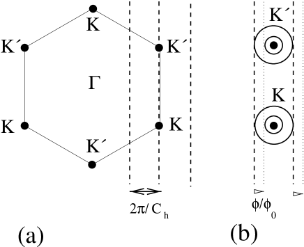
FIG. 3.: (a) Brillouin zone of 2D graphite and typical lines (dashed lines) defining the energy bands near the $K$ points for armchair nanotube. (b) Some equi-energy contours around the $K$ and $K^{\prime}$ points (circles) as well as an illustration of the VHS shifting process. While one VHS gets closer to lower energy (closer to the Fermi energy at the $K$ and $K^{\prime}$ points), the other, initially symmetrical, flows to higher energy.

FIG. 4.: TDoS of an (18,2) tube as a function of the Fermi energy for several values of the magnetic flux, from (a) zero flux to (b) $\phi_{0}/2$ flux, and intermediate cases corresponding to Fig. 2. The inset shows the evolution of the position of three VHSs (as pointed out by arrows) versus normalized magnetic flux.

The TDOS of the semiconducting $(18,2)$ nanotube is also investigated and displays similar features, as exemplified by Fig. 4. The inset gives the shifting of the energy position of the three VHSs, closest to the Fermi level as a function of normalized magnetic flux. An interesting $\phi_{0}/2$ symmetry is clearly seen for semiconducting tubes, as in the former case (Fig. 2) for metallic nanotubes. These interesting effects of the magnetic field on the spectral structure has, to our knowledge, not been explicitly investigated experimentally up to now, but recent progress in the observation of room temperature resonant Raman spectra for purified single-wall nanotubes can disclose fine structure in the DOS, through the enhancement of the intensity of optical absorption at the energies associated with VHSs.[26] Magneto-optical techniques could then provide a possible way to test the above predictions. To that end, we give here the predicted energy position shifts for the VHSs closest to the Fermi energy, which are related to the phase shift induced by magnetic flux variations from 0 to $\phi_{0}/2$ for nanotubes with diameters $d_{1}=1.8$ nm (the largest SWNT made up to now), $d_{2}=6$ nm and $d_{3}=8$ nm (corresponding to typical MWNT outer diameters) and corresponding to $(n,n)$ armchair tubes. The predicted energy position shift is given by

$$\begin{array}[]{rl}\Delta E_{\rm VHS}\left(0,{\displaystyle\frac{1}{2}}\right)=&E_{\rm VHS}^{q=1}\left({\displaystyle\frac{\phi_{0}}{2}}\right)-E_{\rm VHS}^{q=1}(0)\vspace{1mm}\\ =&\gamma_{0}\left(\sin{\displaystyle\frac{3\pi}{2n}}-\sin{\displaystyle\frac{\pi}{n}}\right),\end{array}$$ (11)

which implies $\Delta E_{VHS,1}=173$ meV, $\Delta E_{VHS,2}=52.3$ meV and $\Delta E_{VHS,3}=39.2$ meV, and the corresponding magnetic field strengths at $\phi_{0}/2$ are $B_{1}\sim 200$ T $B_{2}\sim 18$ T, $B_{3}\sim 10$ T, which are within the scope of present experimental capabilities (we take $B=(2\pi\phi_{0})/3(na)^{2}$, and $\phi_{0}=4.1356\times 10^{-15}$ Tm²). Note that the effect of the magnetic field should be observed for individual MWNTs, since the inter-tube coupling for MWNTs is believed to affect the electronic spectrum weakly. Whereas the splitting is universal for all tubes (chiral and achiral), in the most general case, the van Hove singularity shift will depend on the chirality, and on the applied magnetic field strength (not the position of the van Hove singularity). To estimate the corresponding shift, one may proceed in the following manner: given a chiral vector $\vec{\cal C}_{h}=(n,m)$, one calculates the associated vectors $\vec{k}_{\parallel}$ and $\vec{k}_{\perp}$ which are drawn in the Brillouin zone.

This is here illustrated for the $(10,10)$ armchair for which $\vec{k}_{\perp}=(-t_{2}\vec{b}_{1}+t_{1}\vec{b}_{2})/N_{(10,10)}=(\vec{b}_{1}+\vec{b}_{2})/N_{(10,10)}$ with $N_{(10,10)}=40$, the number of hexagons within the unit cell of a (10,10) nanotube, and $\vec{b}_{i}$ the basis vector in reciprocal space (see Ref. [2]), where the direction $\vec{k}_{\perp}$ is found to be perpendicular to the $K-K^{\prime}$-axis (Fig.3), and the spacing between lines is equidistant to a given $K$-point. For the (18,2) chiral nanotube with $N_{(18,2)}=364$, we find $\vec{k}_{\perp}=(11\vec{b}_{1}+19\vec{b}_{2})/N_{(18,2)}$ which defines another direction and spacing. No lines cross at $K$ and $K^{\prime}$ points, and the spacings between two consecutive lines are not equidistant to the $K$-location (in fact the $K$ point always appears to be one-third of the distance between the two lines near the Fermi energy). This affects the splitting, for instance at the field corresponding to half a quantum flux unit, the pattern for the $(18,2)$ nanotube is much less simple than that for the $(10,10)$ nanotube but it can be evaluated systematically.

PERPENDICULAR CASE

For a magnetic field perpendicular to the nanotube axis, the situation is more cumbersome, due to a site-position dependence of the vector potential. No apparent symmetries for the Aharonov–Bohm interferences on the nanotube are found in this case, and indeed, even if semiconducting nanotubes can become metallic with increasing magnetic field strength, non-periodic-oscillations are found, as described below. For $\vec{B}$ normal to the tube axis, one starts from a vector potential, given in the two-dimensional coordinate system $(\vec{\cal C}_{h},\vec{T}$), by

$${\bf\cal A}=\left(0,\frac{B\left|\vec{\cal C}_{h}\right|}{2\pi}\sin\frac{2\pi}{\left|\vec{\cal C}_{h}\right|}{\cal X},0\right).$$ (12)

The effect of the magnetic field is driven by the phase factors introduced into the hopping integrals between two sites ${\bf R_{i}}$ and ${\bf R_{j}}$ (with ${\bf R_{i}}=({\cal X}_{i},{\cal Y}_{i})$, and the phase factor can be deduced from the Peierls substitution as follows, $\Delta\varphi_{{\bf R},{\bf R^{\prime}}}$:

$$\Delta\varphi_{{\bf R},{\bf R^{\prime}}}=\left\{\begin{array}[]{lr}\lx@intercol{\displaystyle\left(\frac{|\vec{\cal C}_{h}|}{2\pi}\right)^{2}B\frac{\Delta{\cal X}}{\Delta{\cal Y}}\left[\cos\frac{2\pi}{|\vec{\cal C}_{h}|}{\cal X}\right.}\hfil\lx@intercol\\ \lx@intercol\hfil{\displaystyle\left.-\cos\frac{2\pi}{|\vec{\cal C}_{h}|}({\cal X}+\Delta{\cal X})\right]}\lx@intercol&(\Delta{\cal X}\neq 0)\\ {\displaystyle\frac{|\vec{\cal C}_{h}|}{2\pi}B\Delta{\cal Y}\sin\frac{2\pi}{|\vec{\cal C}_{h}|}{\cal X}}&(\Delta{\cal X}=0)\\ \end{array}\right.$$ (13)

where $\Delta{\cal X}={\cal X}_{i}-{\cal X}_{j}$ and $\Delta{\cal Y}={\cal Y}_{i}-{\cal Y}_{j}$[2]. In Fig. 1 (b), we show the total density of states (TDOS) at the Fermi level ($E_{F}=0$) as a function of the effective magnetic field defined by $\nu=(L/2\pi\ell_{m})$, where $\ell_{m}=\sqrt{\hbar c/eB}$ is the magnetic length. At low fields, the TDOS of metallic-(9,0) and semiconducting-(10,0) nanotubes at the Fermi level increases with the magnetic field strength. For higher values of magnetic field, our results are in agreement with previous results obtained by exact diagonalization.[2] Also Landau bands are generated for values for which $\nu\geq 2$. The aperiodic fluctuations of the TDOS are stronger at higher fields, with occasional low values of the DOS, reminiscent of a non-zero DOS for the semiconducting nanotubes at the zero-field value.

FIG. 5.: TDoS of a (10,0) nanotube as a function of the Fermi energy for different values of magnetic field, perpendicular to the nanotube axis and with strength $\nu=L/(2\pi\ell_{m})$.

In Fig. 5, several values of $\nu$ are considered for an initially semiconducting nanotube. For $\nu=1$ the radius of the nanotube equals the magnetic length. Landau levels emerge whenever the magnetic length becomes smaller than the nanotube circumference length.[25] Comparison of the case of $\nu=3.5$ in Fig. 5 with the zero-field limit is instructive, since the VHS partition of the spectra has been totally replaced by a Landau level spectrum (Here, one can recognize square-root singularities for the VHSs, and a Lorentzian-shape singularity for the Landau levels). This transition from the VHS-pattern to the Landau-level pattern is, however, more unlikely to be observed experimentally, since its observation requires a very high magnetic field.

III Disorder and magnetic field effects

The effect of Anderson-type disorder on the electronic properties in addition to the presence of a magnetic field is now addressed in order to investigate how disorder alters the VHS-pattern and the metal-insulator transition (MIT), and how disorder qualitatively modifies the localization properties of the nanotubes when the system remains metallic. We consider here only the case of the metallic zigzag nanotube (9,0), but similar results are obtained for other metallic or semiconducting nanotubes. In zero magnetic field, this problem of localization in nanotubes has recently attracted a great deal of attention.[27, 28, 29, 30]

FIG. 6.: TDoS as a function of the energy for $\phi/\phi_{0}=1/2$ and different values of the disorder strength $W$. Thin lines give the zero-disorder case for comparison.

The effect of randomness is considered by taking the site energies of the tight-binding Hamiltonian at random in the interval $[-W/2,W/2]$, with a uniform probability distribution. Accordingly, the strength of the disorder is measured by $W$. Significant fluctuations in the local density of states (LDOS) are found as shown in Fig. 6 (for $\phi/\phi_{0}=1/2$). The TDoS for $W=0.25$ up to $W=2$ ($1/3$ of the total bandwidth) shows that disorder does not modify the gap at the Fermi level, even when the confinement effects disappear (vanishing of VHSs). Disorder obviously leads to a mixing of energy levels which results in a vanishing of the VHS at $W=1$ in our simulations. The gap is more resistant to disorder, even when its strength is as large as $1/3$ the total bandwidth. Thus magnetic effects are not affected by low levels of disorder, which is an interesting result, since it is believed that many defects or sources of weak scattering should be present in real nanotubes. The estimation of the electron mean free path ($\ell_{e}$) in nanotubes is relevant for determining which is the most likely transport regime (ballistic versus diffusive), and further tells us whether or not the conductance should be quantized. While some experiments have observed conductance quantization,[31] others suggest, in contrast, rather short electronic coherence lengths.[16] A calculation of $\ell_{e}$ for armchair nanotubes has been performed using the special symmetries of these systems.[32] Here, we show that a simple recourse to the relaxation time approximation (RTA) in the limit of weak scattering is sufficient to give a fair estimate of $\ell_{e}$ for both chiral or achiral tubes, in qualitative agreement with prior results,[32] demonstrated for the armchair case. Within the RTA, one can write $\ell_{e}=v_{F}\tau_{e}=\hbar v_{F}/(2\Im m\Sigma(E_{F}))$, where $v_{F}$ is an average of the group velocity over the Fermi surface, $\tau_{e}$ is the mean free time, and $\Sigma(E_{F})$ is the self energy due to scattering events. The calculation of the electronic velocity is performed by a linearization of the dispersion relations in the vicinity of the Fermi level. For all metallic nanotubes, one finds to the lowest order of approximation that $\sqrt{\langle v_{k}\rangle^{2}}=v_{F}=\sqrt{3}a\gamma_{0}/2\hbar$ which leads typically to $v_{F}=8.5\times 10^{5}$ ms^-1. On the other hand, in the vicinity of the Fermi level, the density of states is given by

$$\begin{array}[]{rcl}\rho(E)&=&\hbox{Tr}[\delta(E-{\cal H})]\\ &=&{\displaystyle\frac{2}{\tilde{\ell}}\sum_{n}\int dk\delta(k-k_{n})\times\left|\frac{\partial\varepsilon_{nk}}{\partial k}\right|^{-1}}\\ &=&{\displaystyle\frac{2}{\pi\gamma_{0}\sqrt{n^{2}+m^{2}+nm}}}\end{array}$$ (14)

where $\tilde{\ell}=\Delta k|\vec{\cal C}_{h}|/2\pi$ is the volume of $k$-space per allowed $k$ value, divided by the spacing between lines for these allowed values. Equation (14) gives the TDOS per unit length of metallic CNs along the direction of the tube axis. Application of the Fermi golden rule yields $\Im m\Sigma(E_{F})\sim\langle\varepsilon_{i}\rangle^{2}\langle G_{0}(i,i,E_{F})\rangle\sim\pi W^{2}\rho(E_{F})$, where $W$ is the disorder bandwidth and $\langle G_{0}(i,i,E_{F})\rangle$ is the average of the local on-site Green function elements. An estimate of the carrier mean free path (identical for metallic nanotubes with the same radius) is:

$$\ell_{e}\simeq\frac{3\sqrt{3}a{\gamma_{0}}^{2}}{2W^{2}}\sqrt{n^{2}+m^{2}+nm}.$$ (15)

The important result that $\ell_{e}$ is proportional to the nanotube diameter is relevant to the fact that the DOS at the Fermi energy decreases with increasing diameter. Thus, for a given disorder acting as a weak perturbation coupling some eigenstates to others close to Fermi surface, there are less available states to be scattered into, as the tube diameter decreases, yielding an enhancement of the mean free path. For instance for (9,0) and (10,10) CNs, with respective diameters 0.7 nm and 1.37 nm, the corresponding mean-free paths are estimated to be $0.9\mu m$ and $1.8\mu m$, which are much larger than the circumference length and are about the typical length of the systems themselves (for a reasonable disorder $W\sim 0.2eV$ suggested by Ref. [32]). In experiments on SWNTs, or MWNTs in the metallic-like regime (i.e., with an Ohmic temperature dependence of the resistivity), the resistivity should scale as $\rho(d_{nt})\sim 1/d_{nt}$ for a given temperature, where $d_{nt}$ is the tube diameter. It would be interesting to analyze the departure from this law as the diameter of the MWNTs increases, since such departures would indicate a participation of the inner tubes to the measured transport regime. In particular, some activation transport process of inner semiconducting tubes may contribute or not, depending on the temperature, and thus producing superimposed $\rho(d_{nt})\sim\exp(\alpha_{0}d_{nt})$ factors (where $\alpha_{0}$ is a constant). One notes that the Fermi golden rule does not include the quantum interferences which lead to localization. As nanotubes are basically 1D-systems, from their estimated mean free paths, one can estimate the localization lengths at the Fermi level following the Thouless argument.[33] In thin wires, Thouless argued that by writing $R\sim 2\hbar/e^{2}$ for the resistance, there should be a transition to a localized state and an exponential increase of the resistance $R$. Consequently, from the resistance $R=1/G=1/\sigma\times L^{2-D}$ ($G$ is the conductance, $\sigma$ the conductivity and $D$ the dimension of the system), assuming that the conductivity is calculated for a free electron gas in the wire ($\sigma=e^{2}/\hbar\times k_{F}\ell_{e}/3\pi^{2}$), it is straightforward to deduce the localization length $\xi=(2Ak_{F}^{2}\ell_{e})/3\pi^{2}$ (we take $A=L^{D-1}$ as the cross section of the wire and $L=\xi$ as the wire length for which $R=2\hbar/e^{2}$). Rewriting the last expression as $\xi=(A/\lambda_{F}^{2})\ell_{e}$, the localization length $\xi$ is shown to be related to the approximate number of independent electrons (with spatial extension $\sim\lambda_{F}^{2}$, where $\lambda_{F}$ is the Fermi wavelength) which can be accommodated through the cross-section of a single tube times the average mean free path. When confinement effects appear in the direction perpendicular to the cylinder axis, the number of allowed states reduces to the number of bands crossing at the Fermi level (conduction modes), since quantization prevails, and thus $\xi\simeq 2N_{ch}\cdot\ell_{e}$[34], with $N_{ch}=2$, the number of bands crossing the Fermi level for metallic nanotubes. Accordingly, for the $(10,10)$ nanotube, the localization length is estimated to be $\xi\sim 5$ $\mu$m so that it is typically larger or similar to a typical nanotube length and thus no special effects due to localization (insulating regime) are to be expected in SWNTs. With respect to the magnetic field, renormalization group arguments suggest that the localization lengths will be weakly affected by the magnetic field [35] in quasi-1D systems. However, transport properties may be affected by the dephasing magnetic length $\ell_{m}=\sqrt{\hbar/eB}$ which is $\ell_{m}=25.66$ nm or $8$ nm, respectively, for $B=1$Tesla or $B=10$Tesla. Two cases may be distinguished, whenever the mean free path is much larger than the nanotube circumference. Indeed, following Beenakker and Van Houten [36], and noticing that in the case of a nanotube, the cross section of the quantum wire reduces to $\lambda_{F}/2$, the magnetic phase relaxation time $\tau_{B}$ for weak and strong magnetic field limits can be written as follows (for $\lambda_{F}\ll\ell_{e}$):

$$\tau_{B}\simeq\left\{\begin{array}[]{lll}12\left({\displaystyle\frac{\ell_{m}}{\lambda_{F}}}\right)^{2}\tau_{e}&{\rm if}&{\displaystyle\ell_{m}\ll\sqrt{\frac{\lambda_{F}\ell_{e}}{2}}}\\ {\displaystyle 128\left(\frac{\ell_{m}^{4}}{\lambda_{F}^{3}\ell_{e}}\right)\tau_{e}}&{\rm if}&{\displaystyle\ell_{m}\gg\sqrt{\frac{\lambda_{F}\ell_{e}}{2}}}\\ \end{array}\right.$$ (18)

So for the considered $(9,0)$ and $(10,10)$ tubes, we find that $\lambda_{F}\ell_{e}/2\sim 18.24$nm and $25.8$nm respectively (we take $\lambda_{F}=0.74$nm[12] and $W=0.2078$eV[32]). Thus for $B=1$Tesla we conclude that $\ell_{m}\simeq\sqrt{\lambda_{F}\ell_{e}/2}$ which is an intermediate situation between low and strong magnetic field, and no analytical expression of $\tau_{B}$ can be deduced, whereas $B=10$Tesla is closer to the strong magnetic field limit where magnetic phase relaxation can be estimated analytically by

$$\tau_{B}={\displaystyle\frac{12\gamma_{0}\hbar}{(\lambda_{F}W)^{2}}}\ell_{m}^{2}\sqrt{n^{2}+m^{2}+nm}$$ (19)

which gives for the $(10,10)$ armchair nanotube a dephasing rate of $\tau_{B}\sim 2.8\times 10^{-11}s$. This means that for an $(10,10)$ armchair tube, the electronic phase is randomized by a 10 Tesla magnetic field roughly every 30 ps, which indicates that in the strong field limit, the dephasing rate due to a magnetic field is just a few times the mean free times (we find $\tau_{B}/\tau_{e}\sim 3.14$ with the aforementioned parameters), so that $\tau_{B}$ should strongly contribute to damp the quantum interferences in the weak localization regime. Actually, both the mean free time and the magnetic dephasing rate scale linearly with diameter. Inelastic dephasing rates due to electron-phonon coupling have been recently evaluated by Suzuura and Ando[37], and an interesting chirality-dependent dominant inelastic backscattering mechanism (breathing, stretching versus twisting[2]) was revealed. From their analytical estimate of the electron-phonon inelastic scattering rate ($\tau_{el-ph}$), in the $(10,10)$ armchair case, one finds at room temperature $\tau_{el-ph}\simeq 1.34\times 10^{-5}s$ which is much larger than former estimated coherence times (elastic mean free time and magnetic dephasing rate), so that one deduces that the main damping effect for the weak localization regime is likely to be dominated by the magnetic field strength.

Finally, with regard to the experimental results[16], one notices that if electronic transport is conveyed only by the outer shell of a metallic-like nanotube, as the magnetic field tends to decrease the TDoS at discrete values of the magnetic field corresponding to $(2n+1)/2\phi_{0}$ with integer $n$, an increase of resistance may follow from increasing the magnetic field. However, the short electronic coherence lengths that are observed in a magnetic field, the negative magnetoresistance and the $\phi_{0}/2$ Aharonov–Bohm oscillatory pattern are unlikely to be fully due to spectral effects (on the density of states), and a calculation of diffusion coefficients is mandatory to account for interferences between propagating electronic pathways in the nanotube structure. A recent study of the Kubo formula has been performed in Ref. [38] and gives a geometrical explanation for the enhanced backscattering in MWNTs.

- [1] S. Iijima, Nature 354, 56 (1991).
- [2] R. Saito, G. Dresselhaus, and M. S. Dresselhaus, Physical Properties of Carbon Nanotubes (Imperial College Press, London, 1998).
- [3] Y. Zhang et al., Science 285 (1999) 1719.
- [4] H. T. Soh et al., Appl. Phys. Lett. 75 (1999) 627.
- [5] J. C. Charlier, T. W. Ebbesen and Ph. Lambin, Phys. Rev. B. 53 (1996) 11108.
- [6] S. G. Louie, S. Froyer and M.L. Cohen, Phys. Rev. B 26 (1982) 1738.
- [7] Y. Saito, S. Uemura and K. Hamaguchi, J. Appl. Phys. 37 (1998) L346.
- [8] J. W. G. Wildöer, L. C. Venema, A. G. Rinzler, R. E. Smalley and C. Dekker, Nature 391 (1998) 59.
- [9] R. Martel, T. Schmidt, H. Shea, T. Hertel and Ph. Avouris, Appl. Phys. Lett. 73, 2447 (1998).
- [10] S. J. Tans, R. M. Verschueren, and C. Dekker, Nature 393, 49 (1998).
- [11] L. Venema et al., Nature 396 (1999) 52.
- [12] A. Rubio et al., Phys. Rev. Lett. 82, 3520 (1999).
- [13] R. Saito, G. Dresselhaus and M. S. Dresselhaus, Phys. Rev. B 61 (2000) 2981.
- [14] L. Langer et al., Phys. Rev. Lett. 76, 479 (1996).
- [15] C. Naud, G. Faini, D. Mailly and H. Pascard, C. R. Acad. Sci. Paris, t. 327, Serie II b (1999).
- [16] A. Bachtold et al., Nature 397, 673 (1999).
- [17] A. Fujiwara et al., Phys. Rev. B. 60, 13492 (1999).
- [18] H. Ajiki and T. Ando, J. Phys. Soc. of Japan 62, 1255 (1993). J. P. Lu, Phys. Rev. Lett. 74, 1123 (1995).
- [19] C. H. Olk and J. P. Heremans, J. Mater. Res. 9 (1994) 259.
- [20] P. Kim, T. Odom and J. L. Huang, Phys. Rev. Lett. 82 (1999) 1225. Phys. Rev. Lett. 82, 1225 (1999).
- [21] S. Roche and R. Saito, Phys. Rev. B59 (1999) 5242.
- [22] T. W. Odom et al., Nature 391 (1998) 62.
- [23] M. Ichida, J. Phys. Soc. Japan 68 (1999) 3131.
- [24] J. M. Mintmire and C. T. White, Phys. Rev. Lett. 81, 2506 (1998).
- [25] H. Ajiki and T. Ando, Journ. Phys. Soc. of Japan 65, 505 (1996).
- [26] H. Kataura et al., Synth. Met. 103 (1999) 2555.
- [27] L. Chico, L. X. Benedict, S. G. Louie and M. L. Cohen, Phys. Rev. B 54, 2600 (1996).
- [28] M. P. Anatran and T. R. Govindan, Phys. Rev. B 58, 4882 (1998).
- [29] T. Kostyrko, M. Bartkowiak, and G. D. Mahan, Phys. Rev. B 60, 10735 (1999)
- [30] K. Harigaya, Phys. Rev. B 60 1452 (1999).
- [31] S. Frank, P. Poncharal, Z. L. Wang and W. A. de Heer, Science 280 (1998) 1744.
- [32] C. T. White and T. N. Todorov, Nature 393 (1998) 240.
- [33] D. J. Thouless, Phys. Rev. Lett. 39 (1977) 1167.
- [34] K. B. Efetov and A. I. Larkin, Sov. Phys. JETP 58, 444 (1983).
- [35] I. V. Lerner and Y. Imry, Europhys. Lett. 29 (1995) 49.
- [36] C. W. J. Beenakker and H. van Houten, Phys. Rev. B 38, 3232 (1988).
- [37] H. Suzuura and T. Ando, Mol. Cryst. Liq. Cryst. (in press).
- [38] S. Roche et. al., submitted.