Non–monotonous crossover between capillary condensation and interface localisation/delocalisation transition in binary polymer blends

Abstract

Within self–consistent field theory we study the phase behaviour of a symmetric binary $AB$ polymer blend confined into a thin film. The film surfaces interact with the monomers via short range potentials. One surface attracts the $A$ component and the corresponding semi–infinite system exhibits a first order wetting transition. The surface interaction of the opposite surface is varied as to study the crossover from capillary condensation for symmetric surface fields to the interface localisation/delocalisation transition for antisymmetric surface fields. In the former case the phase diagram has a single critical point close to the bulk critical point. In the latter case the phase diagram exhibits two critical points which correspond to the prewetting critical points of the semi–infinite system. The crossover between these qualitatively different limiting behaviours occurs gradually, however, the critical temperature and the critical composition exhibit a non-monotonic dependence on the surface field.

1 Introduction

We study the phase behaviour of a symmetric binary mixture confined into a slit–like pore. The shift of the critical point for symmetric film surfaces[1] (capillary condensation) has been studied extensively. The unmixing transition approaches the critical temperature of the infinite system for thick films. Below the critical temperature the coexisting phases differ in their composition at the center of the film. More recently, novel types of phase transitions have been studied in the case of antisymmetric surface fields,[2-6] i.e., one surface attracts the $A$ component of a symmetric mixture in exactly the same way the opposite surface attracts the $B$ component. Close to the critical temperature in the bulk, enrichment layers of the components gradually form at the surfaces and stabilise an interface at the center of the film (soft–mode phase). It is only close to the temperature[3] of the second order wetting transition in the semi–infinite system that the symmetry is spontaneously broken and the interface is located at either surface. Upon increasing the film thickness the temperature of this interface localisation/delocalisation transition converges to the wetting temperature rather than the critical temperature of the bulk, and the interpretation of the transition in terms of a thin film critical critical point or a wetting transition in the limit of large film thickness has been discussed.[7] The effect of an external field (i.e., gravity) has been explored.[8] Analytical approaches and simulations have considered systems with second order wetting transitions[3, 6] in the semi–infinite system or the behaviour at bulk coexistence[5, 9] only. This has excluded a possible interplay between phase behaviour and prewetting, which might alter the topology of the phase diagram in thin films,[10, 11] from consideration.

In this Letter we revisit the interface localisation/delocalisation transition for a first order wetting transition in the corresponding semi–infinite system and explore the crossover from the interface localisation/delocalisation transition to capillary condensation upon varying the interaction $\Lambda_{2}$ at one surface. The interaction $\Lambda_{1}$ at the other surface is kept constant. This is the first systematic theoretical study of boundary conditions which are neither strictly symmetric nor antisymmetric. It is clearly pertinent to the interpretation of experiments as the idealized limiting cases are never strictly realized. Our calculations yield information about the range of asymmetry where the behaviour characteristic of the symmetric and antisymmetric boundary conditions is observable, and we explore the dependence of the topology of the phase diagrams on the surface interactions. Both the phase diagram as a function of the intensive variables incompatibility and chemical potential as well as the binodals are discussed.

2 Self–consistent field calculations

We calculate the phase behaviour of a confined $AB$ mixture within the self-consistent field theory of Gaussian polymers.[12-14]Polymer mixtures in confined geometries are interesting for many applications (e.g., coating, lubrication), and consequentially have attracted abiding recent attention.[15] In these systems the soft mode phase mentioned above has been experimentally studied.[16] Thus we focus on these systems, although we believe that our results carry over to other confined mixtures at least qualitatively. We consider a film with volume $V_{0}=\Delta_{0}\times L\times L$. $\Delta_{0}$ denotes the film thickness, while $L$ is the lateral extension of the film. The density at the film surfaces decreases to zero in a boundary region of width $\Delta_{w}$ according to[17]

$$\Phi_{0}(x)=\left\{\begin{array}[]{ll}\frac{1-\cos\left(\frac{\pi x}{\Delta_{w}}\right)}{2}&\mbox{{; $0\leq x\leq\Delta_{w}$}}\\ 1&\mbox{{; $\Delta_{w}\leq x\leq\Delta_{0}-\Delta_{w}$}}\\ \frac{1-\cos\left(\frac{\pi(\Delta_{0}-x)}{\Delta_{w}}\right)}{2}&\mbox{{; $\Delta_{0}-\Delta_{w}\leq x\leq\Delta_{0}$}}\end{array}\right.$$ (1)

where $\Phi_{0}$ denotes the ratio of the monomer density and the value $\rho$ in the middle of the film. The thickness $\Delta$ of an equivalent film with constant monomer density $\rho$ is $\Delta=\Delta_{0}-\Delta_{w}$. We choose $\Delta_{w}=0.15R_{e}$,[17] where $R_{e}$ is the end–to–end distance. Both surfaces interact with the monomer species via a short range potential $H$:

$$H(x)=\left\{\begin{array}[]{ll}\frac{4\Lambda_{1}R_{e}\left\{1+\cos\left(\frac{\pi x}{\Delta_{w}}\right)\right\}}{\Delta_{w}}&\mbox{{; $0\leq x\leq\Delta_{w}$ }}\\ 0&\mbox{{; $\Delta_{w}\leq x\leq\Delta_{0}-\Delta_{w}$}}\\ \frac{4\Lambda_{2}R_{e}\left\{1+\cos\left(\frac{\pi(\Delta_{0}-x)}{\Delta_{w}}\right)\right\}}{\Delta_{w}}&\mbox{{; $\Delta_{0}-\Delta_{w}\leq x\leq\Delta_{0}$}}\end{array}\right.$$ (2)

$H>0$ is attractive for the $A$ monomers and repulsive for the $B$ species. The normalisation of the surface fields $\Lambda_{1}$ and $\Lambda_{2}$, which act on the monomers close to the left and the right surface, is chosen such that the integrated interaction energy between the surface and the monomers is independent of the width of the boundary region $\Delta_{w}$.

$A$ and $B$ polymers contain $N$ monomers and are structurally symmetric. The polymer conformations $\{{\bf r}_{\alpha}(\tau)\}$ determine the microscopic $A$ monomer density $\hat{\Phi}_{A}({\bf r})=\frac{N}{\rho}\sum_{\alpha=0}^{n_{A}}\int_{0}^{1}{\rm d}\tau\times$
$\delta\left({\bf r}-{\bf r}_{\alpha}(\tau)\right)$, where the sum runs over all $n_{A}$ $A$ polymers in the system and $0\leq\tau\leq 1$ parameterises the contour of the Gaussian polymer. A similar expression holds for $\hat{\Phi}_{B}({\bf r})$. With this definition the semi–grandcanonical partition function takes the form:

$${\cal Z} \sim\sum_{n_{A}=1}^{n}\frac{e^{+\Delta\mu n_{A}/2k_{B}T}}{n_{A}!}\;\;\frac{e^{-\Delta\mu n_{B}/2k_{B}T}}{n_{B}!} \int{\cal D}_{A}[{\bf r}]{\cal P}_{A}[{\bf r}]\int{\cal D}_{B}[{\bf r}]{\cal P}_{B}[{\bf r}]\;\delta\left(\Phi_{0}-\hat{\Phi}_{A}-\hat{\Phi}_{B}\right)$$ (3)

$$\;\times\;\exp\left(-\rho\int{\rm d}^{3}{\bf r}\left\{\chi\hat{\Phi}_{A}\hat{\Phi}_{B}-H(\hat{\Phi}_{A}-\hat{\Phi}_{B}\right\}\right)$$

where $n=n_{A}+n_{B}$ and $\Delta\mu$ represents the exchange potential between $A$ and $B$ polymers. The functional integral ${\cal D}$ sums over all conformations of the polymers, and ${\cal P}[{\bf r}]\sim\exp\left(-\frac{3}{2R_{e}^{2}}\int_{0}^{1}{\rm d}\tau\;\left(\frac{{\rm d}{\bf r}}{{\rm d}\tau}\right)^{2}\right)$ denotes the statistical weight of a non–interacting Gaussian polymer. The second factor enforces the monomer density profile to comply with Eq.(1) (incompressibility). The Boltzmann factor in the partition function incorporates the thermal repulsion between unlike monomers and the interactions between monomers and surfaces. The strength of the repulsion is described by the Flory–Huggins parameter $\chi$.

In mean field approximation the free energy is obtained as the extremum of the functional:

$$\frac{{\cal G}[W_{A},W_{B},\Phi_{A},\Phi_{B},\Xi]}{nk_{B}T}\equiv+\;\ln\frac{n}{V_{0}}-\;\ln{\cal Q}+\;\frac{1}{V}\int{\rm d}^{3}{\bf r}\;\;\chi N\Phi_{A}\Phi_{B}-HN\left\{\Phi_{A}-\Phi_{B}\right\}$$

$$-\;\frac{1}{V}\int{\rm d}^{3}{\bf r}\;\;\left\{W_{A}\Phi_{A}+W_{B}\Phi_{B}\right\}+\Xi\left\{\Phi_{0}-\Phi_{A}-\Phi_{B}\right\}$$ (4)

with respect to its five arguments. ${\cal Q}_{A}$ denotes the single chain partition function:

$${\cal Q}_{A}[W_{A}]=\frac{1}{V_{0}}\int{\cal D}_{1}[{\bf r}]{\cal P}_{1}[{\bf r}]\;\;e^{-\int_{0}^{1}{\rm d}\tau\;W_{A}({\bf r}(\tau))}$$ (5)

a similar expression holds for ${\cal Q}_{B}$, and ${\cal Q}=\exp(\Delta\mu/2k_{B}T){\cal Q}_{A}+\exp(-\Delta\mu/2k_{B}T){\cal Q}_{B}$.

The values of $W_{A},W_{B},\Phi_{A},\Phi_{B},\Xi$ which extremize the free energy functional are denoted by lower–case letters and satisfy the self-consistent set of equations

$$w_{A}({\bf r})=\chi N\phi_{B}({\bf r})-H({\bf r})N+\xi({\bf r})\qquad\mbox{and}\qquad\phi_{A}({\bf r})=-\frac{V}{{\cal Q}}\frac{{\cal DQ}_{A}}{{\cal D}w_{A}({\bf r})}$$ (6)

$\Phi_{0}({\bf r})=\phi_{A}({\bf r})+\phi_{B}({\bf r})$, and similar expressions for $\phi_{B}$ and $w_{B}$.

To calculate the monomer density we employ the end segment distribution $q_{A}({\bf r},t)$

$$q_{A}({\bf r},\tau)=\int_{0}^{\tau}{\cal D}_{1}[{\bf r}]{\cal P}_{1}[{\bf r}]\delta({\bf r}-{\bf r}(\tau))e^{-\int_{0}^{\tau}{\rm d}t\;w_{a}({\bf r}(t))}$$ (7)

It satisfies the diffusion equation:

$$\frac{\partial q_{A}({\bf r},\tau)}{\partial\tau}=\frac{R_{e}^{2}}{6}\triangle q_{A}({\bf r},\tau)-w_{A}({\bf r})q_{A}({\bf r},\tau)$$ (8)

Then, the $A$ monomer density and the single chain partition can be calculated via

$$\phi_{A}({\bf r})=\frac{Ve^{\Delta\mu/2k_{B}T}}{V_{0}{\cal Q}}\int_{0}^{1}{\rm d}\tau\;q_{A}({\bf r},\tau)q_{A}({\bf r},1-\tau)\qquad\mbox{and}\qquad{\cal Q}_{A}=\frac{1}{V_{0}}\int{\rm d}^{3}{\bf r}\;q_{A}({\bf r},1)$$ (9)

We expand the spatial dependence of the densities and fields in a set of orthonormal functions $\{f_{k}(x)=\sqrt{2}\sin(\pi kx/\Delta_{0})\}$ with $k=1,2,\cdots$.[13, 17] This procedure results in a set of non–linear equations which are solved by a Newton–Raphson–like method. We use up to 80 basis functions and achieve a relative accuracy $10^{-4}$ in the free energy. For symmetric boundary fields only components with an odd index $k$ are non–zero. Substituting the extremal values of the densities and fields into the free energy functional (4) we calculate the free energy $G$ of the different phases. At coexistence the two phases have equal semi–grandcanonical potential.

3 Results

The phase boundaries as a function of the surface fields are presented in Fig.1. First, we consider the antisymmetric boundary condition $\Lambda_{1}N=-\Lambda_{2}N=0.5$. One half of the phase diagram is enlarged in the inset. If we reduce the temperature along the symmetry axis of the phase diagram $\phi=1/2$, an interface is stabilized at the center of the film for $\chi N<\chi_{\rm triple}N$, and at $\chi_{\rm triple}N$ we encounter a first order interface localisation/delocalisation transition at which the interface jumps discontinuously to one of the two surfaces. At this triple point phases with compositions $\phi_{\rm triple}$, $1/2$ and $1-\phi_{\rm triple}$ coexist. This behaviour for $\Delta\mu=0$ has been confirmed by computer simulations of Ising models.[6, 9]

(a)

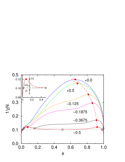
(b)

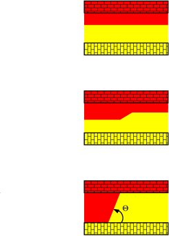
$(u)$

$(m)$

$(l)$

Fig. 1.–: (a) Binodals for $\Delta_{0}=2.6R_{e}$ and $\Lambda_{1}N=0.5$. $\Lambda_{2}N$ varies as indicated in the key. The dashed curve shows the location of the critical points. Filled circles mark critical points, open circles/dashed horizontal lines denote three phase coexistence for $\Lambda_{2}N=-0.3675$ and $-0.5$. The inset presents part of the phase boundary for antisymmetric boundaries. (b) Schematic temperature dependence for antisymmetric boundaries. The three profiles correspond to the situations (u),(m), and (l) in the inset of (a).

For all other compositions in the range $[\phi_{\rm triple}:1-\phi_{\rm triple}]$, however, one encounters two transitions upon cooling. Consider cooling at $\phi_{\rm triple}<\phi<1/2$ as indicated by the arrow in the inset. At high temperatures enrichment layers gradually form at the surfaces. Slightly below the critical temperature of the bulk an interface is stabilized which separates a thin $A$–rich layer at one surface from a thicker $B$–rich layer at the opposite surface (cf. Fig.1b upper panel). Laterally, the system is homogenous (soft–mode phase) and an $AB$ interface runs parallel to the surfaces. Upon cooling, we first encounter a phase separation into lateral regions with a thin and a thick $A$–rich layer(cf. Fig.1b middle panel). This phase coexistence is the analogy of the prewetting line in a semi–infinite system. Since the coexistence involves only finite layer thicknesses it also persists in a thin film, provided the film thickness is sufficiently large. The different layer thicknesses correspond to different compositions of the film and give rise to two symmetric coexistence regions. This prediction has not yet been observed in computer simulations[6, 9] or experiments.[16, 18] Upon further cooling, we encounter a second transition at $\chi_{\rm triple}N$ where the two phase coexistences merge and the system laterally segregates into $A$–rich and $B$–rich regions(cf. Fig.1b lower panel). For temperatures far below the triple temperature the interface between the coexisting phases runs straight across the film. The angle between the interface and the surface corresponds to the contact angle $\Theta$ of droplets in the semi–infinite system. Upon increasing the film thickness the triple temperature approaches the wetting transition temperature, the two coexistence regions become narrower and converge to the prewetting lines, and the critical temperature of the film tends to the prewetting critical temperature of the semi–infinite system.[19]

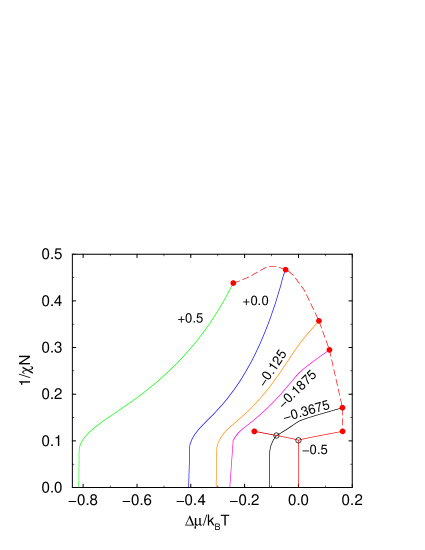
Fig. 2.–: Coexistence curves in the $\chi N$–$\Delta\mu$ plane. $\Lambda_{2}N$ varies according to the key. Parameters and symbols as in Fig.1. The “quasi–prewetting” lines for $\Delta\mu<0$ and $\Lambda_{2}N=-0.3675$ and $-0.5$ are indistinguishable, because they are associated with the prewetting behaviour of the surface with interaction $\Lambda_{1}N=+0.5$.

The phase coexistence in terms of incompatibility $\chi N$ and exchange potential $\Delta\mu$ is shown in Fig.2. Although the Hamiltonian of the system is symmetric with respect to the exchange $A\rightleftharpoons B$, phase coexistence occurs at $\Delta\mu=0$ only below the triple temperature. At $\chi_{\rm triple}N$ the coexistence curve bifurcates and the branches move away from the symmetry axis. The two coexistence lines resemble the prewetting lines which correspond to the first order wetting transitions at the two surfaces.

At low temperatures $\chi\gg\chi_{\rm triple}$ the two coexisting phases are almost pure and the coexistence value of the chemical potential is given by $\Delta\mu_{\rm coex}/k_{B}T=-4(\Lambda_{1}+\Lambda_{2})NR_{e}/\Delta$. Upon increasing $\Lambda_{2}$ this value shifts to more negative values. Only for large film thickness the two phase region on the $B$–rich side of the phase diagram remains.[10, 11] For thin films, however, $\Delta\mu_{\rm coex}$ is shifted to negative values which are eventually smaller than the chemical potential of the prewetting critical point at the surface which attracts $A$ (cf. Fig.2). For the parameters chosen this occurs roughly around $\Lambda_{2}N\approx-0.2$. In this case the two phase region on the $B$–rich side as well as the associated critical point disappears upon increasing $\Lambda_{2}$ further.

The critical point on the $A$–rich side of the phase diagram shifts to higher temperatures upon increasing $\Lambda_{2}$ similar to the prewetting at the corresponding surface. Note that $\chi_{\rm wet}N\approx 24(\Lambda_{2}N)^{2}$ for strong segregation.[11] Although the film surfaces favor (on average) the $A$ component of the mixture, the critical point occurs at $\Delta\mu>0$ for $\Lambda_{2}N\stackrel{{\scriptstyle<}}{{~{}}}-0.25$. Around $\phi=1/2$ or $\Delta\mu_{\rm coex}=0$ the $B$–rich binodal shows a concave curvature, which is the remanent of the wetting transition at the surface which favours $B$. Upon increasing $\Lambda_{2}$ to positive values this feature disappears, of course.

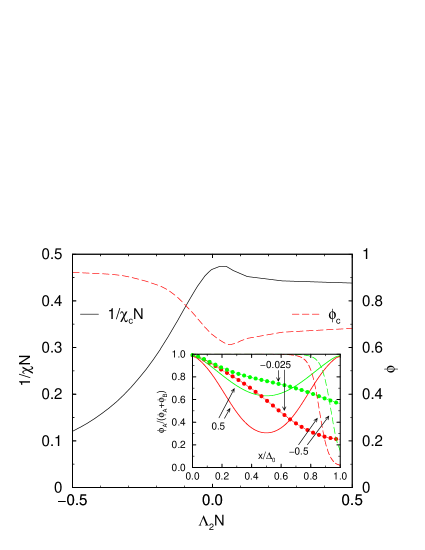
Fig. 3.–: Dependence of the critical temperature (left axis) and density (right axis) on the surface field $\Lambda N_{2}$. $\Lambda_{1}N=0.5$ and $\Delta_{0}=2.6R_{e}$. The inset presents the composition profiles of the coexisting phases $3\%$ below the critical temperature for $\Lambda_{2}N=0.5$ (solid line), $-0.025$ (dotted line) and $-0.5$ (dashed line).

For an almost neutral surface $\Lambda_{2}N\approx 0$ the critical temperature passes through a maximum and the critical temperature of the capillary condensation is approached from above.[20] The surface field dependence of the critical temperature and critical density is investigated in Fig.3. This non-monotonic behaviour of the critical temperature and density can be rationalised as follows: For $\Lambda_{2}=\Lambda_{1}$ the composition profiles of the two coexisting phases close to the critical point are symmetric (c.f. Fig.3 inset). It is the difference in the composition at the center which distinguishes between the phases and vanishes at the critical point. Decreasing $\Lambda_{2}$ we reduce the influence of the surfaces, and the critical temperature increases and the critical composition decreases, respectively, as both tend towards their bulk values.[21] For large negative values of $\Lambda_{2}$ the transition is qualitatively different. It is associated with the prewetting transition, i.e., the profiles of the coexisting phases resemble a profile across an interface and it is the location of the interface which distinguishes the two phases (c.f. Fig.3 inset). Decreasing $\Lambda_{2}$ shifts the wetting transition to lower temperatures and higher $A$ content. The gradual crossover between the two distinct behaviours occurs around $\Lambda_{2}\approx 0$.[22] The corresponding profiles are included into Fig.3 (inset). In both phases the composition at the surface favouring $A$ is almost saturated and the composition decreases to a value larger or smaller than 1/2 at the almost neutral surface. Upon approaching the critical point the composition difference at the neutral surface vanishes. This is similar to the capillary condensation mechanism for $\Lambda_{2}>0$. Both profiles, however, can also be perceived as very broad interfaces (with a width comparable to the film thickness) with different centers. This resembles the prewetting–like behaviour for $\Lambda_{2}<0$.

4 Discussion

In summary, we have explored the unusual dependence of the phase behaviour of a confined symmetric mixture on the surface fields. For nearly antisymmetric surface fields which are strong enough to produce a first order wetting transition our mean field calculations predict two coexistence regions which correspond to the prewetting transition at either surface. We vary the surface interactions from antisymmetric to symmetric and the critical temperature(composition) passes through a maximum(minimum) when one surface is almost neutral. We expect the qualitative dependence of the phase diagram on the surface fields to be generic. Fluctuations, which are not included in the mean field calculations, impart 2D Ising rather than mean field behaviour to the critical points. Their importance is, however, restricted to a narrow region around the critical point in the limit of strong interpenetration $\rho R_{e}^{3}/N\gg 1$. Capillary waves increase the range of the effective interaction[4] between interface and surface by a factor $1+\omega/2$ where $\omega=k_{B}T/4\pi\xi^{2}\sigma$. $\xi$ and $\sigma$ denote the correlation length and interfacial tension between the coexisting bulk phases, respectively. Simulations[11] indicate that $1/\omega\sim\sqrt{\chi N}f(\chi N)\rho R_{e}^{3}/N$, where the scaling function $f(\chi N)$ approaches a constant value for $\chi N\to\infty$. Since the wetting transition in binary polymer blends is typically first order and occurs at strong segregation,[11] the capillary parameter $\omega$ is small. Experiments[16, 18] on polymer blends have explored the phase behaviour in confined geometry, and these systems as well as computer simulations might prove convenient for testing our predictions.

We are currently exploring the thickness dependence of the phase diagram for antisymmetric surfaces within the self–consistent field theory and a Landau–Ginzburg approach.[19] Contrary to the behaviour close to a second order wetting transition, we find that the triple point approaches the temperature of the first order wetting transition from above upon increasing the film thickness. The transition between first and second order interface localisation/delocalisation transition and the behaviour at the tricritical point will be elucidated.

***

It is a pleasure to thank E. Reister and F. Schmid for helpful discussions. Financial support was provided by the DFG under grant Bi314/17 within the Priority Program “Wetting and Structure Formation at Interfaces”, the VW Stiftung, and PROALAR2000.

References

- [1] M.E. Fisher, H. Nakanishi, J.Chem.Phys. 75, 5857 (1981); H. Nakanishi, M.E. Fisher, ibid 78, 3279 (1983).
- [2] F. Brochard–Wyart, P.-G. de Gennes, Acad.Sci. Paris 297, 223 (1983).
- [3] A.O. Parry, R. Evans, Phys.Rev.Lett. 64, 439 (1990).
- [4] A.O. Parry, R. Evans, Physica A181, 250 (1992).
- [5] M.R. Swift et al., Europhys.Lett. 14, 475 (1991).
- [6] K. Binder et al., Phys.Rev.Lett. 74, 298 (1995); E.V. Albano et al., Surf.Sci. 223, 151 (1989).
- [7] J.O. Indekeu et al., Phys.Rev.Lett. 66, 2174 (1991); A.O. Parry, R. Evans, ibid 66, 2175 (1991).
- [8] J. Rogiers, J.O. Indekeu, Europhys.Lett. 24, 21 (1993); E. Carlon, A. Drzewinski, Phys.Rev.Lett. 79, 1591 (1997).
- [9] A.M. Ferrenberg et al., Phys.Rev. E58, 3353 (1998).
- [10] D. Nicolaides, R. Evans, Phys.Rev. B39, 9336 (1989); R. Evans, U.M.B. Marconi, Phys.Rev. A32, 3817 (1985).
- [11] M. Müller, K. Binder, Macromolecules 31, 8323 (1998).
- [12] J. Noolandi, K.M. Hong, Macromolecules 14, 727 (1981).
- [13] M.W. Matsen, Phys.Rev.Lett. 74, 4225 (1995); M.W. Matsen, M. Schick, ibid 72, 2660 (1994).
- [14] F. Schmid, J.Phys.Condens.Matter 10, 8105, (1998).
- [15] K. Binder, Adv.Polymer Sci 138, 1 (1999); A. Budkowski, Adv.Polymer Sci 148, 1 (1999).
- [16] T. Kerle et al., Phys.Rev.Lett. 77, 1318 (1996).
- [17] M.W. Matsen, J.Chem.Phys. 106, 7781 (1997); T. Geisinger et al.. ibid 111, 5241 (1999).
- [18] M. Sferrazza et al, Phys.Rev.Lett. 81, 5173 (1998); ibid 78, 3693 (1997).
- [19] M. Müller et al., Physica A 279, 188 (2000), and (preprint, 2000).
- [20] More general, the shift in the critical temperature can be described by a finite–size scaling ansatz of the form: and where and denote the bulk correlation length and the surface gap exponent in mean field theory.[1] Our calculations indicate a non–monotonic behaviour of the scaling function .
- [21] The critical point for completely neutral surfaces occurs at and , which is very close to the bulk critical point .
- [22] This behaviour differs from qualitative considerations.[6]