[

Two-Dimensional Modeling of Soft Ferromagnetic Films

Abstract

We examine the response of a soft ferromagnetic film to an in-plane applied magnetic field. Our theory, based on asymptotic analysis of the micromagnetic energy in the thin-film limit, proceeds in two steps: first we determine the magnetic charge density by solving a convex variational problem; then we construct an associated magnetization field using a robust numerical method. Experimental results show good agreement with the theory. Our analysis is consistent with prior work by van den Berg and by Bryant and Suhl, but it goes much further; in particular it applies even for large fields which penetrate the sample.

]

Soft ferromagnetic films are of great interest both for applications and as a model physical system. Their sensitive response to applied magnetic fields makes them useful for the design of many devices, including sensors and magnetoelectronic memory elements [1]. Therefore soft thin films have been the object of much experimental and computational study [2]. Their relatively simple domain structures and significant hysteresis make such films a convenient paradigm for analyzing the microstructural origin of magnetic hysteresis [3].

Most current modeling of soft thin films is based on direct micromagnetic simulation [4]. This is demanding due to the long-range nature of dipolar interactions, and the necessity of resolving several small length scales simultaneously. Numerical simulation is surely the right tool for the quantitative study of hysteresis and dynamic switching [5]. However it is natural to seek a more analytical understanding of the equilibrium configurations. The origin of domain patterns is intuitively clear: they arise through a competition between the magnetostatic effects (which favor pole-free in-plane magnetization) and the applied field (which tends to align the magnetization). A 2D model based on this intuition was developed by van den Berg [6] in the absence of an applied field, and extended by Bryant and Suhl [7] to the case of a sufficiently weak in-plane applied field. In van den Berg’s model (VDBM) magnetic domain patterns are represented using 2D, unit-length, divergence-free vector fields, determined using the method of characteristics; the caustics where characteristics meet are domain walls. In Bryant and Suhl’s model (BSM), the presence of a weak applied field is accounted for through an electrostatic analogy: the “charges” associated with the magnetic domain pattern should be such as to expel the applied field from the interior of the sample, as occurs in an electrical conductor. The domain patterns predicted by BSM have been observed experimentally [8]. The electrostatic analogy is restricted, however, to sufficiently small applied fields: since the magnetization vector has a constrained magnitude, the field generated by its divergence cannot be arbitrarily large. Therefore the BSM breaks down at a critical field strength beyond which the external field penetrates the sample.

This Letter extends and clarifies the models of van den Berg and of Bryant and Suhl. Our extension is two-fold: we permit large applied fields which penetrate the sample, and we replace the method of characteristics with a robust numerical scheme. Our clarification is also two-fold: we identify the regime in which these 2D models are valid, and explain their relation to classical micromagnetics. To assess the extended model, we compare its predictions to experiments on Permalloy thin film elements with square cross-section. The agreement between theory and experiment is remarkable, even in the field penetration regime. At the heart of our approach is an asymptotic analysis of the micromagnetic energy in the thin-film limit. The lowest-order terms lead to constraints such as $m_{3}=0$, while the second-order term sets the charge density. Wall energies and anisotropy contribute only at higher order. The higher-order terms are not irrelevant: they are the source of magnetic hysteresis. Our analysis indicates, however, that certain quantities should have little or no hysteresis – namely the charge density, the region of field penetration, and the magnetization in the penetrated region.

The free-energy functional of micromagnetics in units of $J_{s}^{2}L^{3}/2\mu_{0}$ is

$$E_{d}(m) = (\kappa d)^{2}\int_{\Omega_{d}}|\nabla m|^{2}dx+Q\int_{\Omega_{d}}\varphi(m)dx$$ (1)

$$+ \int_{{I\hskip-4.0ptR}^{3}}|h_{d}|^{2}dx-2\int_{\Omega_{d}}h^{\prime}_{e}\cdot mdx\,.$$ (2)

Here $m$ is the magnetization (in units of the saturation magnetization $J_{s}$), a unit vector field defined on the film $\Omega_{d}$ with cross section $\omega$ and thickness $d$, where all lengths are measured in units of a typical lateral dimension $L$ (the diameter for $\omega$ a circle, the edge-length for $\omega$ a square). Moreover, $\kappa$ is the ratio between Bloch line width $D_{BL}$ and the film thickness, where $D_{BL}=(2\mu_{0}A/J_{s}^{2})^{\frac{1}{2}}$, with $A$ the exchange constant, measures the strength of the exchange energy relative to that of dipolar interactions; $Q$ is the quality factor measuring the relative strength of the magnetic anisotropy $\varphi$; $h_{d}$ is the stray field in units of $J_{s}/\mu_{0}$, whose norm squared gives the magnetostatic energy density; $h^{\prime}_{e}$ is the applied field in units of $J_{s}/\mu_{0}$, which we assume to be uniform and parallel to the film’s cross section. In what follows, a prime will always denote a two-dimensional field or operator.

For $d\ll 1$ a hierarchical structure emerges in the energy landscape of (1), see Table I. Variations of $m$ of order $1$ along the thickness direction $x_{3}$ give rise to an exchange energy per unit area (of the cross section) of order $\kappa^{2}d$. An out–of–plane component $m_{3}$ of order one determines a magnetostatic contribution per unit area of order $d$. The component of the in-plane magnetization $m^{\prime}$ orthogonal to the lateral boundary $\partial\omega$ of the film’s cross section $\omega$ leads to a magnetostatic contribution of order $d^{2}\ln\frac{1}{d}$ per unit length. The same mechanism penalizes jumps $\left[m^{\prime}\cdot\nu^{\prime}\right]$ of the normal component of the magnetization across a line of discontinuity of $m^{\prime}$ with normal $\nu^{\prime}$. These lines of discontinuity arise by approximating domain walls as sharp interfaces. At order $d^{2}$ we find the magnetostatic energy per unit area due to surface “charges” proportional to the in-plane divergence ${\rm div}^{\prime}m^{\prime}$. Finally, the energy per unit length of a Néel or asymmetric Bloch wall and the energy of a single vortex are indicated in the table. In the regime

$$H^{\prime}_{e}=\frac{h^{\prime}_{e}}{d}\sim 1,\quad\frac{Q}{d}\ll 1,\quad d\ll\kappa^{2}\ll\frac{1}{d\ln\left(\frac{1}{d}\right)}\,,$$ (3)

the highest-order terms penalizing $m_{3}$, $\frac{\partial m}{\partial x_{3}}$ and $[m^{\prime}\cdot\nu^{\prime}]$ become hard constraints, while the energetic cost of anisotropy, of the wall type of minimal energy [9], and of vortices become higher-order terms. The energy is thus determined, at principal order, by the competition between the aligning effect of $H^{\prime}_{e}$ and the demagnetizing effects due to ${\rm div}^{\prime}m^{\prime}$.

TABLE I.: Scaling of various energy sources

$\frac{\partial m}{\partial x_{3}}$	$\kappa^{2}d$
$m_{3}$	$d$
$\left[m^{\prime}\cdot\nu^{\prime}\right]$	$\ln(\frac{1}{d})\,d^{2}$
${\rm div}^{\prime}m^{\prime}$	$d^{2}$
external field energy	$h^{\prime}_{e}\,d$
anisotropy energy	$Q\,d$
asymmetric Bloch wall	$\kappa^{2}\,d^{2}$
Néel wall	$(\ln(\frac{1}{\kappa^{2}\,d}))^{-1}\,d^{2}$
vortex	$\ln(\frac{1}{\kappa\,d})\,\kappa^{2}\,d^{3}$

In view of this separation of energy scales in the regime (3), we propose the following reduced theory. We call an in–plane vector field $m^{\prime}(x^{\prime})$ on $\omega$ “regular” if it satisfies $\left[m^{\prime}\cdot\nu^{\prime}\right]=0$ across all possible discontinuity lines and at $\partial\omega$. Our reduced theory states that the magnetization $m^{\prime}(x^{\prime})$ minimizes

$$E(m^{\prime})=\int_{{I\hskip-4.0ptR}^{3}}|H_{d}|^{2}\,dx-2\int_{\omega}H^{\prime}_{e}\cdot m^{\prime}\,dx^{\prime},$$ (4)

where $H_{d}(x)=-\nabla U$ is determined by

$$\nabla^{2}U = 0\;\;\mbox{in}\;{I\hskip-4.0ptR}^{3}\;\mbox{outside of}\;\omega,$$

$$\left[\frac{\partial U}{\partial x_{3}}\right] = {\rm div}^{\prime}m^{\prime}\;\;\mbox{on}\;\omega\,,$$

among all regular in-plane vector fields $m^{\prime}$ of unit length

$$|m^{\prime}|=1\;\;\mbox{in}\;\omega.$$ (5)

Our formula for the induced field $H_{d}$ is naturally consistent with that commonly used for 2D micromagnetic simulations [10].

We now make two crucial observations. The first is that the functional $E$ depends on $m^{\prime}$ only via the surface charge $\sigma=-{\rm div}^{\prime}m^{\prime}$, and it is strictly convex in $\sigma$. Indeed, $\int_{{I\hskip-4.0ptR}^{3}}|H_{d}|^{2}\,dx$ is a quadratic functional of $\sigma$ and an integration by parts shows that $\int_{\omega}H_{e}^{\prime}\cdot m^{\prime}\,dx^{\prime}$ is a linear functional of $\sigma$. The second observation is that the set of regular in–plane vector fields of unit length and with given surface charge is large in the following sense: For any regular $m^{\prime}_{0}$ of at most unit length, that is

$$|m^{\prime}_{0}|\leq 1\;\;\mbox{in}\;\omega,$$ (6)

there exist many regular $m^{\prime}$ of unit length with the same surface charge: ${\rm div}^{\prime}m^{\prime}={\rm div}^{\prime}m^{\prime}_{0}$. Indeed, we may write $m^{\prime}=\nabla^{\perp}\psi+m^{\prime}_{0}$ where $\nabla^{\perp}\psi=(-\partial\psi/\partial x_{2},\partial\psi/\partial x_{1})$ and the continuous function $\psi(x^{\prime})$ on $\omega$ solves the boundary value problem

$$|\nabla^{\perp}\psi+m^{\prime}_{0}| = 1\;\;\mbox{in}\;\omega,$$ (7)

$$\psi = 0\;\;\mbox{on}\;\partial\omega.$$ (8)

Condition (6) ensures the solvability of this boundary value problem. One can generate many solutions by imposing the additional condition $\psi=0$ on an arbitrary curve contained in $\omega$.

These observations have two important consequences. First, the minimizer of the reduced energy $E$ is not uniquely determined. Indeed, according to our first observation, $E$ depends only on the surface charge, and according to our second observation, a regular in–plane vector field of unit length is not uniquely determined by its surface charge.

The second consequence is that the surface charge and thus the stray field are uniquely determined. Indeed, according to our first observation, $E$ is a strictly convex function of the surface charge, and according to our second observation, the set of surface charges which can be generated by regular in–plane vector fields of unit length is convex. (This is true despite the fact that the set of regular in–plane vector fields with unit length is not convex.)

Any minimizer $m^{\prime}$ of (4,5) satisfies the Euler-Lagrange equation

$$H^{\prime}_{d}+H^{\prime}_{e}=\lambda\,m^{\prime}\;\;\mbox{in}\;\omega,$$ (9)

where $\lambda(x^{\prime})$ is the Lagrange multiplier associated with the pointwise constraint (5). Since $H_{d}$ is uniquely determined, the region $\{H^{\prime}_{d}+H^{\prime}_{e}\not=0\}$ of $\omega$ where the external field is not expelled from the sample is uniquely determined. Within this penetrated region, $m^{\prime}$ is also uniquely determined in view of (9).

There is a finite critical field strength $H_{crit}$, in the following sense: when the applied field is subcritical $\lambda\equiv 0$ and the field is completely expelled from the sample, whereas when it is supercritical $\lambda$ is nonzero somewhere and the field penetrates in that part of the sample. The critical field strength depends on the geometry of $\omega$ — for a circular disk of diameter $1$, its value is $1$. Further analysis indicates that there can be no walls (discontinuity lines of $m^{\prime}$) in the penetrated region. Moreover the penetrated region must meet the boundary of $\omega$.

To derive quantitative predictions from our reduced model (4,5), we proceed in two steps. The first step minimizes (4) among all regular in–plane vector fields $m^{\prime}_{0}$ of length less than or equal to $1$. Recall that replacing (5) by (6) does not change the minimum energy; therefore the $m^{\prime}_{0}$ obtained this way has the correct reduced energy, though it typically violates (5). The second step postprocesses $m^{\prime}_{0}$ by solving (7,8) to obtain another minimizer $m^{\prime}$ of unit length. This $m^{\prime}$ is the desired magnetization.

The first step is a convex (though degenerate) variational problem. We solve it using an interior point method [11]: the convex constraint is enforced by adding to the physical energy $E$ a small multiple $t$ of a self–concordant barrier $B$. The unique stationary point of the strictly convex $E+tB$ is computed by Newton’s method; it serves as an initial guess for the minimizer of $E+t^{\prime}B$, where $t^{\prime}<t$. The parameter $t$ is slowly decreased by multiplicative increments. Within Newton’s method, the Hessian of $E+tB$ is inverted by a preconditioned conjugate gradient method. The magnetostatic part of the Hessian is evaluated with the help of FFT. This is a robust procedure.

For the second step, we recall that the solution of (7,8) is not unique. However there is a special solution $\psi$, known as the “viscosity solution”, which has special mathematical properties [12]. It is robust and can be computed efficiently using the “level set method” [13]. This is what we compute.

Our numerical scheme selects — automatically and robustly — one of the many minimizers $m^{\prime}$. The selection principle implicit in this scheme is the same as the one proposed by Bryant and Suhl. It appears to pick a minimizer with as few walls as possible. Thus it is not unlike the more physical selection mechanism of minimizing wall energy, represented as a higher-order correction to (4) [14].

Figure 1 shows the predictions of our numerical scheme for a square film of edge-length one, subject to a monotonically increasing field applied along the diagonal. To check our predictions, we have observed the response of two ac-demagnetized Permalloy (Ni₈₁Fe₁₉, $J_{s}=1.0$ T) square samples of edge lengths $L=$ 30 and 60 $\mu$m and thicknesses $D=$ 40 and 230 nm, respectively, in a digitally enhanced Kerr microscope. The observed domain patterns are given in Figures 2, 3 where the field intensity $h_{e}$, measured in Tesla, is scaled according to

$$H=\frac{L}{D}\frac{h_{e}}{J_{s}}.$$ (10)

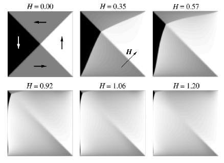
FIG. 1.: Predictions of the theory: gray-scale plots of the vertical component of magnetization.

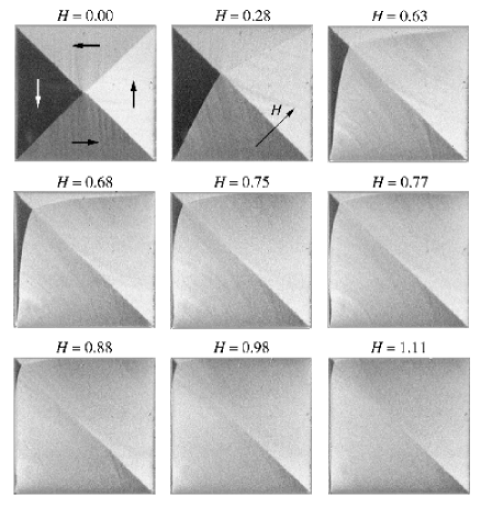
FIG. 2.: Permalloy films: $L=60$ $\mu$m, $D=230$ nm.

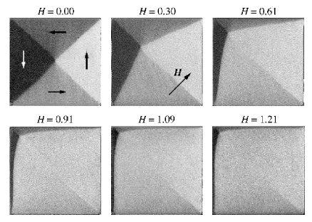
FIG. 3.: Permalloy films: $L=30$ $\mu$m, $D=40$ nm.

Figure 4 examines more closely the predictions of our theory for $|H^{\prime}_{e}|$ close to $H_{crit}$. We have superimposed on each gray-scale plot the level curves of the potential $v$ of the penetrated field, defined by

$$-\nabla v=H^{\prime}_{d}+H^{\prime}_{e}\,.$$

Regions where the field lines concentrate are regions where $\nabla v\neq 0$, i.e., where the external field has penetrated the sample. Within them, (9) implies that $m^{\prime}$ is parallel to $\nabla v$ . Our theory predicts that the penetrated region must meet the boundary of the sample and that $m^{\prime}$ can have no walls in the penetrated region. The pictures confirm this, and show quite clearly that two apparently independent phenomena – the expulsion of the domain walls from the interior of the sample and the penetration of the external field – are in fact two manifestations of the same event.

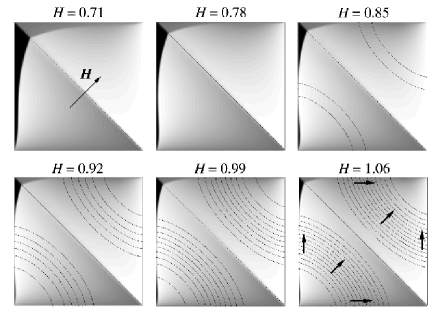
FIG. 4.: The transition between expulsion and penetration regimes. In the last picture, arrows indicate the magnetization direction.

In summary, our model describes the response of a soft ferromagnetic thin film to an applied magnetic field. It determines the micromagnetic energy to principal order, and certain associated physical quantities that should have little or no hysteresis — the charge density, the region of field penetration, and the magnetization in the penetrated region. In addition our approach provides a specific magnetization pattern which is consistent with experimental observation and may well be the ground state. Of course, the magnetization of a soft thin film is not uniquely determined by the applied field: the multiplicity of metastable states is a primary source of hysteresis. Our approach does not provide a model for hysteresis or a classification of stable structures — this would seem to require analysis of higher-order terms in the micromagnetic energy.

We thank S. Conti for valuable discussions.

REFERENCES

- [1] see e.g. Physics Today 48 (April 1995), special issue on magnetoelectronics.
- [2] A. Hubert and R. Schäfer, Magnetic Domains (Springer, Berlin–Heidelberg–New York, 1998).
- [3] G. Bertotti, Hysteresis in Magnetism (Academic Press, San Diego, 1998).
- [4] see e.g. J. Fidler et al., J. Magnetism Magn. Mat. 175, 193 (1997); J.G. Zhu et al., J. Appl. Phys. 81, 4336 (1997).
- [5] R.H. Koch et al., Phys. Rev. Lett. 81, 4512 (1998); Yu Lu et al., Phys. Rev. B 60, 7352 (1999);
- [6] H.A.M. van den Berg, J. Appl. Phys. 60, 1104 (1986) and IBM J. Res. Develop. 33, 540 (1989)
- [7] P. Bryant and H. Suhl, Appl. Phys. Lett. 54, 78 and 2224 (1989) and J. Appl. Phys. 66, 4329 (1989)
- [8] M. Rührig et al., IEEE Trans. Magnetics 26, 2807 (1990).
- [9] Note that (3) probes a range of film thicknesses over which different wall types are to be expected, see ref. [2]. Typical values for Permalloy are and nm. For a circular element with diameter m and thickness nm we have and .
- [10] J.L. Blue and M.R. Scheinfein, IEEE Trans. Magnetics 27, 4778 (1991).
- [11] R.J Vanderbei, Linear Programming: Foundations and Extensions (Kluwer, Boston, 1996).
- [12] L.C. Evans Partial Differential Equations (American Mathematical Society, Providence, 1998), Section 10.1.
- [13] J.A. Sethian, Level Set Methods (Cambridge University Press, 1996).
- [14] P. Aviles and Y. Giga, Proc. Roy. Soc. Edinburgh A 126, 923 (1996); W. Jin and R. V. Kohn, J. Nonlinear Science, to appear.