Trapped condensates of atoms with dipole interactions

Abstract

We discuss in detail properties of trapped atomic condensates with anisotropic dipole interactions. A practical procedure for constructing anisotropic low energy pseudo potentials is proposed and justified by the agreement with results of numerical multi-channel calculations. The time dependent variational method is adapted to reveal several interesting features observed in numerical solutions of condensate wave function. Collective low energy shape oscillations and their stability inside electric fields are investigated. Our results shed new light into macroscopic coherence properties of interacting quantum degenerate atomic gases.

03.75.Fi, 05.30.-d, 32.80.Pj

I introduction

The recent success in atomic Bose-Einstein condensation (BEC) [1, 2, 3] has stimulated great research activities into trapped quantum gases [4]. To a remarkable degree, a single condensate wave function of the macroscopically occupied ground state, described by the nonlinear Schrödinger equation (NLSE) [5], captures all essential features of its coherence properties [6]. In fact, one of the key diagnosis features for BEC, the reversed aspect ratio of a free expanding condensate, is described purely by the condensate wave function [7, 8]. In the standard treatment for the condensate wave function of interacting atoms, realistic inter-atomic potential $V(\vec{R})$ is often not directly used. Instead, a contact pseudo potential, $u_{0}\delta(\vec{R})$, obtained under the so-called shape independent approximation (SIA) [9] is used. Such an idealization results in tremendous simplification, yet to date, SIA has worked remarkably well as verified by both theoretical calculations and experimental observations [4, 10, 11].

Currently available degenerate quantum gases are cold and dilute, the interaction is therefore dominated by s-wave collisions, described by a single atomic parameter: $a_{\rm sc}$, the s-wave scattering length, if the inter-atomic potential is isotropic and short ranged (decaying fast than $-1/R^{3}$ asymptotically). The complete scattering amplitude is then isotropic and energy-independent, given by $f(\vec{k},\vec{k}^{\prime})=-4\pi a_{\rm sc}$ for collisions of incoming momentum $\vec{k}$ state scattering into $\vec{k}^{\prime}$.

One of the attractive features of atomic degenerate gases lies at effective means for control of the atom-atom interaction [12, 13, 14]. Indeed, very recently several groups have successfully implemented Feschbach resonance [15, 16], thus enabling a control knob on $a_{\rm sc}$ through the changing of an external magnetic field. Other physical mechanisms also exist for modifying atom-atom interactions, e.g. the shape resonance as proposed in [17]. In an external electric field, inter atomic potential is modified by the addition of an anisotropic (induced) dipole interaction.

Although anisotropically interacting fermi system has been an important area of study, e.g. liquid ³He [18] and d-wave paired high $T_{c}$ superconductors [19]. Its bosonic counterpart has not been studied in great detail. In particular, we are not aware of any systematic approach for constructing an anisotropic pseudo potential [9].

For bosonic systems, another related topic is the condensate stability. Under the SIA, the scattering length takes a positive or negative value, corresponding to repulsive or attractive interactions. When $a_{\rm sc}<0$ occurs, self-interaction leads to a collapse of BEC in dimensions higher than 1 [20], thus the resulting condensate is limited by a critical number of particles [21]. Anisotropic dipole interactions, on the other hand, are more complicated as both attractive and repulsive interactions arise along different directions. We note that several recent investigations have studied efforts of non-local interactions on condensate stability [22, 23].

In this paper, we study properties of trapped BEC of atoms with dipole interactions [24], arising from either external electric field (induced) or permanent magnetic moments [25]. We propose a practical method for constructing anisotropic pseudo potentials that can also be extended for investigation of polar molecular BEC [27, 28]. This paper is organized as following. We first briefly review the usual pseudo-potential approximation under the SIA. In Sec. II we describe and justify in detail a procedure for constructing effective low energy pseudo-potentials of anisotropic interactions. In Sec. III we provide our numerical procedure for solving the NLSE with anisotropic dipole interactions. Particular emphasis is put on the careful treatment of the singular origin of dipole interactions. We also present and discuss results from selected numerical calculations. To explain the stability region as well as the interesting aspect ratios observed from our numerical calculations, we perform in Sec. IV an analytic time dependent variational calculation. We compare the results obtained with direct numerical solutions of NLSE. Finally we conclude.

II formulation

For $N$ trapped spinless bosonic atoms in a potential $V_{t}(\vec{r})$, the second quantized Hamiltonian is given by

$${\cal H} = \int\!d\vec{r}\,\hat{\Psi}^{{\dagger}}(\vec{r})\left[-\frac{\hbar^{2}}{2M}\nabla^{2}+V_{t}(\vec{r})-\mu\right]\hat{\Psi}(\vec{r})$$ (1)

$$+ \frac{1}{2}\int\!d\vec{r}\int\!d\vec{r}^{\prime}\hat{\Psi}^{{\dagger}}(\vec{r})\hat{\Psi}^{{\dagger}}(\vec{r}^{\prime})V(\vec{r}-\vec{r}^{\prime})\hat{\Psi}(\vec{r}^{\prime})\hat{\Psi}(\vec{r}),$$ (2)

where $\hat{\Psi}(\vec{r})$ and $\hat{\Psi}^{{\dagger}}(\vec{r})$ are atomic (bosonic) annihilation and creation fields. The chemical potential $\mu$ guarantees the atomic number $\hat{N}=\int d\vec{r}\,\hat{\Psi}^{{\dagger}}(\vec{r})\hat{\Psi}(\vec{r})$ conservation.

The bare potential $V(\vec{R})$ in (2) needs to be renormalized for a meaningful perturbation calculation [9]. The usual treatment is based an effective interaction obtained by a resummation of certain classes of interaction diagrams [29, 30, 31]. Physically the SIA can be viewed as a valid low energy and low density renormalization scheme, one simply replaces the bare potential $V(\vec{R})$ by a pseudo potential $u_{0}\delta(\vec{R})$ whose first order Born scattering amplitude reproduces the complete scattering amplitude ($-a_{\rm sc}$). This gives $u_{0}=4\pi\hbar^{2}a_{\rm sc}/M$.

When an electric field is introduced along the positive z axis, an additional term

$$V_{E}(\vec{R}) =u_{2}{Y_{20}(\hat{R})\over R^{3}},$$ (3)

appears in the atom-atom interaction [17], where $u_{2}=-4\sqrt{(\pi/5)}\,\alpha(0)\alpha^{*}(0){\cal E}^{2}$. $\alpha(0)$ is the atomic polarizability, and ${\cal E}$ denotes the electric field strength. As was shown before [17], this modification results in a completely new form for the low-energy scattering amplitude

$$f(\vec{k},\vec{k}^{\prime})\Big{|}_{k=k^{\prime}\to 0}=4\pi\sum_{lm,l^{\prime}m^{\prime}}t_{lm}^{l^{\prime}m^{\prime}}({\cal E})Y_{lm}^{*}({\hat{k}})Y_{l^{\prime}m^{\prime}}({\hat{k}^{\prime}}),$$ (4)

with $t_{lm}^{l^{\prime}m^{\prime}}({\cal E})$ the reduced T-matrix elements. They are all energy independent and act as generalized scattering lengths. The anisotropic $V_{E}$ causes the dependence on both incident and scattered directions: $\hat{k}$ and $\hat{k}^{\prime}=\hat{R}$.

We therefore propose a general (energy-independent) anisotropic pseudo potential constructed according to

$$V_{\rm eff}(\vec{R})=u_{0}\delta(\vec{R})+\sum_{l_{1}>0,m_{1}}\gamma_{l_{1}m_{1}}{Y_{l_{1}m_{1}}(\hat{R})\over R^{3}},$$ (5)

whose first Born amplitude is

$$f_{\rm Born}(\vec{k},\vec{k}^{\prime})=-(4\pi)^{2}a_{\rm sc}Y_{00}^{*}(\hat{k})Y_{00}(\hat{k}^{\prime})-{M\over 4\pi\hbar^{2}}\sum_{l_{1}m_{1}}\gamma_{l_{1}m_{1}}(4\pi)^{2}\sum_{lm}\sum_{l^{\prime}m^{\prime}}{\cal T}_{lm}^{l^{\prime}m^{\prime}}(l_{1},m_{1})Y_{lm}^{*}(\hat{k})Y_{l^{\prime}m^{\prime}}(\hat{k}^{\prime}),$$ (6)

with ${\cal T}_{lm}^{l^{\prime}m^{\prime}}(l_{1},m_{1})=(i)^{l+l^{\prime}}{\cal R}_{l}^{l^{\prime}}I_{lm}^{l^{\prime}m^{\prime}}(l_{1},m_{1}).$ Both

$$I_{lm}^{l^{\prime}m^{\prime}}(l_{1}m_{1}) =\langle Y_{l^{\prime}m^{\prime}}|Y_{l_{1}m_{1}}|Y_{lm}\rangle$$ (12)

$$=(-1)^{m}\sqrt{(2l+1)(2l^{\prime}+1)(2l_{1}+1)\over 4\pi}\left(\begin{array}[]{ccc}l&l^{\prime}&l_{1}\\ -m&m^{\prime}&m_{1}\end{array}\right)\left(\begin{array}[]{ccc}l&l^{\prime}&l_{1}\\ 0&0&0\end{array}\right),$$

and

$${\cal R}_{l}^{l^{\prime}} =\int_{0}^{\infty}dR\,{1\over R}j_{l}(kR)j_{l^{\prime}}(k^{\prime}R)$$ (14)

$$={\pi\over 8}\eta^{l}{\Gamma({l+l^{\prime}\over 2})\over\Gamma({3+l^{\prime}-l\over 2})\Gamma(l+{3\over 2})}\ _{2}F_{1}\left({-1-l^{\prime}+l\over 2},{l+l^{\prime}\over 2},l+{3\over 2};\eta^{2}\right),$$

can be computed analytically. The $1/R^{3}$ form in Eq. (5) assures all ${\cal R}_{l}^{l^{\prime}}$ to be $k=k^{\prime}$ independent (easily seen by a change of variable to $x=kR$ in the integral). Putting

$$f_{\rm Born}(\vec{k},\vec{k}^{\prime})=f(\vec{k},\vec{k}^{\prime}),$$ (15)

i.e. requiring the Bohn amplitude from the pseudo potential Eq. (5) to be the same as the numerically computed value $f(\vec{k},\vec{k}^{\prime})$, one can solve for all $\gamma_{l_{1}m_{1}}({\cal E})$ from known $t_{lm}^{l^{\prime}m^{\prime}}({\cal E})$ [17, 32]. This reduces to a set of (under determined) linear equations

$$-{M\over 4\pi\hbar^{2}}\sum_{l_{1}m_{1}}\gamma_{l_{1}m_{1}}(4\pi){\cal T}_{lm}^{l^{\prime}m^{\prime}}(l_{1},m_{1})\equiv t_{lm}^{l^{\prime}m^{\prime}},$$ (16)

for all ($lm$) and ($l^{\prime}m^{\prime}$) with $l,l^{\prime}\neq 0$, and separately $a_{\rm sc}({\cal E})=-t_{00}^{00}({\cal E})$.

Considerable simplification arises further for bosons (fermions) as only even (odd) $(l,l^{\prime})$ terms are needed to match in (16). Figure 1 displays the result of field dependent $a_{\rm sc}({\cal E})$ ⁴¹K atoms in the triplet electron spin state. Note the spikes of shape resonances. The Born amplitude for the dipole term $V_{E}$ is

$$f_{\rm Born}(\vec{k},\vec{k}^{\prime}) =u_{2}{M\over 4\pi\hbar^{2}}(4\pi)^{2}{\cal T}_{00}^{20}\sum_{lm,l^{\prime}m^{\prime}}\overline{\cal T}_{lm}^{l^{\prime}m^{\prime}}Y_{lm}^{*}(\hat{k})Y_{l^{\prime}m^{\prime}}(\hat{k}^{\prime}),$$ (17)

with ${\cal T}_{00}^{20}=-0.023508$. $\overline{\cal T}_{lm}^{l^{\prime}m^{\prime}}={\cal T}_{lm}^{l^{\prime}m^{\prime}}(2,0)/{\cal T}_{00}^{20}$ are independent of electric field ${\cal E}$ within the perturbative Born approximation as tabulated below.

TABLE I.: $\bar{\cal T}_{lm}^{l^{\prime}m^{\prime}}=t_{lm}^{l^{\prime}m^{\prime}}({\cal E})/t_{00}^{20}({\cal E})$ for small $(l,l^{\prime})$.

$(lm),(l^{\prime}m^{\prime})$	(00)	(20)	(40)	(60)	(80)
(00)	0	1	0	0	0
(20)	1	-0.63889	0.14287	0	0
(40)	0	0.14287	-0.17420	0.05637	0
(60)	0	0	0.05637	-0.08131	0.03008
(80)	0	0	0	0.03008	-0.04707

We find that away from regions of shape resonances to be discussed elsewhere [32], all numerically computed $t_{lm}^{l^{\prime}m^{\prime}}({\cal E})$ values, large enough to justify their inclusions, are actually all proportional to ${\cal E}^{2}$. Thus, we could rewrite $f(\vec{k},\vec{k}^{\prime})$ as

$$f(\vec{k},\vec{k}^{\prime})=(4\pi)t_{00}^{20}({\cal E})\sum_{lm,l^{\prime}m^{\prime}}\overline{t}_{lm}^{l^{\prime}m^{\prime}}Y_{lm}^{*}({\hat{k}})Y_{l^{\prime}m^{\prime}}({\hat{k}^{\prime}}),$$ (18)

with scaled quantities $\overline{t}_{lm}^{l^{\prime}m^{\prime}}=t_{lm}^{l^{\prime}m^{\prime}}({\cal E})/t_{00}^{20}({\cal E})$ now all being constants. We have since computed (numerically) for several alkali metal isotopes, our results for $\overline{t}_{lm}^{l^{\prime}m^{\prime}}$ are tabulated below.

TABLE II.: $\overline{t}_{lm}^{l^{\prime}m^{\prime}}$ for ⁷Li.

$(lm),(l^{\prime}m^{\prime})$	(00)	(20)	(40)	(60)	(80)
(00)	0	1.0	0.0	0.0	0.0
(20)	1.0	-0.63	0.14	0.0	0.0
(40)	0.0	0.14	-0.17	0.057	0.0
(60)	0.0	0.0	0.057	-0.080	0.031
(80)	0.0	0.0	0.0	0.031	-0.044

TABLE III.: $\overline{t}_{lm}^{l^{\prime}m^{\prime}}$ for ³⁹K.

$(lm),(l^{\prime}m^{\prime})$	(00)	(20)	(40)	(60)	(80)
(00)	0	1.0	0.0	0.0	0.0
(20)	1.0	-0.64	0.14	0.0	0.0
(40)	0.0	0.15	-0.17	0.085	0.0
(60)	0.0	0.0	0.085	-0.127	0.047
(80)	0.0	0.0	0.0	0.047	-0.074

TABLE IV.: $\overline{t}_{lm}^{l^{\prime}m^{\prime}}$ for ⁴¹K.

$(lm),(l^{\prime}m^{\prime})$	(00)	(20)	(40)	(60)	(80)
(00)	0	1.0	0.0	0.0	0.0
(20)	1.0	-0.64	0.14	0.0	0.0
(40)	0.0	0.14	-0.17	0.057	0.0
(60)	0.0	0.0	0.057	-0.081	0.030
(80)	0.0	0.0	0.0	0.030	-0.047

TABLE V.: $\overline{t}_{lm}^{l^{\prime}m^{\prime}}$ for ⁸⁵Rb.

$(lm),(l^{\prime}m^{\prime})$	(00)	(20)	(40)	(60)	(80)
(00)	0	1.0	0.0	0.0	0.0
(20)	1.0	-0.64	0.14	0.0	0.0
(40)	0.0	0.14	-0.17	0.056	0.0
(60)	0.0	0.0	0.056	-0.081	0.030
(80)	0.0	0.0	0.0	0.030	-0.047

TABLE VI.: $\overline{t}_{lm}^{l^{\prime}m^{\prime}}$ for ⁸⁷Rb.

$(lm),(l^{\prime}m^{\prime})$	(00)	(20)	(40)	(60)	(80)
(00)	0	1.0	0.0	0.0	0.0
(20)	1.0	-0.64	0.15	0.0	0.0
(40)	0.0	0.15	-0.17	0.056	0.0
(60)	0.0	0.0	0.056	-0.079	0.032
(80)	0.0	0.0	0.0	0.032	-0.045

The agreement between the first order Born approximation and the multi-channel scattering calculations is remarkable. We estimate the numerical scattering results to be accurate to a few percent (except for ³⁹K), independent of atoms being bosons (even $l,l^{\prime}$) or fermions (odd $l,l^{\prime}$). Only bosonic results are being considered in this paper. This is displayed by noticing the agreement between Table I ($\sim$ a few per cent) with Table II-VI. This interesting observation applies for all bosonic alkali triplet states: ⁷Li, ^39,41K, and ^85,87Rb, for up to a field strength of $3\times 10^{6}$ (V/cm) [17, 32] computed by us. Physically, this implies the effect of $V_{E}$ is perturbative when ${\cal E}$ remains small (in a.u.). For the convenience of further discussions, we tabulate polarizabilities of selected atoms in Table VII.

TABLE VII.: Atomic polarizabilities in (a.u.).

	H	Li	Na	K	Rb
$\alpha(0)$	4.5	159.2	162	292.8	319.2

What is remarkable is the fact that ${\cal T}_{00}^{20}({\cal E})$ and $t_{00}^{20}({\cal E})$ also agree in absolute values [17] except for a slight difference (1-6%). They are calculate below and tabulated in VIII.

$$u_{2}{M\over 4\pi\hbar^{2}}(4\pi)^{2}{\cal T}_{00}^{20} =-16\pi\sqrt{\pi\over 5}{\cal T}_{00}^{20}\alpha^{2}{\cal E}^{2}{M\over\hbar^{2}}$$ (20)

$$=1718\times\overline{M}\overline{\alpha}^{2}\overline{\cal E}^{2}a_{0},$$

where all overlined quantities are in atomic units (a.u.).

TABLE VIII.: Comparison of numerical values of $u_{2}{M\over 4\pi\hbar^{2}}(4\pi)^{2}{\cal T}_{00}^{20}$ with $-(4\pi)t_{00}^{20}({\cal E})$, the cause of the slight difference is unclear but within numerical errors.

	Born	Multichannel
atom	$u_{2}{M\over 4\pi\hbar^{2}}(4\pi)^{2}{\cal T}_{00}^{20}(a_{0})$	$-(4\pi)t_{00}^{20}({\cal E})(a_{0})$
7Li	$3.040\times 10^{8}{\overline{\cal E}}^{2}$	$3.238\times 10^{8}{\overline{\cal E}}^{2}$
39K	$5.713\times 10^{9}{\overline{\cal E}}^{2}$	$5.699\times 10^{9}{\overline{\cal E}}^{2}$
41K	$6.006\times 10^{9}{\overline{\cal E}}^{2}$	$5.99\times 10^{9}{\overline{\cal E}}^{2}$
85Rb	$1.486\times 10^{10}{\overline{\cal E}}^{2}$	$1.474\times 10^{10}{\overline{\cal E}}^{2}$
87Rb	$1.495\times 10^{10}{\overline{\cal E}}^{2}$	$1.512\times 10^{10}{\overline{\cal E}}^{2}$

An important parameter in our discussion is the ratio between $u_{2}$ and $u_{0}$. Since the results from first order Born approximation and the multichannel calculations are about the same, one can write this ratio as

$$c({\cal E})=-{u_{2}\over u_{0}}=\gamma{\cal E}^{2},$$ (21)

where $\gamma\simeq 1.748\times 10^{-17}\overline{\alpha}^{2}\overline{M}/\overline{a}_{\rm sc}$ and ${\cal E}$ is in unit of V/cm. The $\gamma$ values for selected atoma are tabulated in Table IX.

TABLE IX.: Values of parameter $\gamma$ for selected atoms with their field free (${\cal E}=0$) scattering lengths.

	H	7Li	23Na	41K	87Rb
$\gamma\,(\times 10^{-13})$	$2.9\times 10^{-3}$	$-1.1$	$2.0$	$2.2$	$15.0$

Most atoms possess permanent magnetic dipoles. With alkali metals, the magnetic dipole mainly originates from valance electron spin, typically measured in units of Bohr magneton. It is therefore interesting to compare electric dipole interactions with magnetic dipole interactions. The dipole interaction strength between atoms of a permanent magnetic dipole $\mu$ is

$$\mu^{2} ={\overline{\mu}}^{2}\mu_{B}^{2}$$ (23)

$$=1.331\times 10^{-5}{\overline{\mu}}^{2}e^{2}a_{0}^{2},$$

with $\mu_{B}$ the unit of Bohr magneton. For induced electric dipoles, the interaction strength is

$$\alpha^{2}{\cal E}^{2}={\overline{\alpha}}^{2}{\overline{\cal E}}^{2}e^{2}a_{0}^{2}.$$ (24)

A typical heavy alkali atom has ${\overline{\alpha}}\sim 200$, thus for which a 1 ($\mu_{B}$) magnetic moment corresponds to an effective electric field of $3.3\times 10^{-5}$ (a.u.), or $1.7\times 10^{5}$ (V/cm). Atoms with large magnetic moments effectively simulates induced dipole interactions at a high value of equivalent electric field [25].

As can be concluded from comparing listed data in all tables, we can approximate Eq. (5) by keeping only the $l_{1}=2$, $m_{1}=0$ term to achieve a satisfactory level of accuracy. Thus away from shape resonances we take

$$V_{\rm eff}(\vec{R})=u_{0}\delta(\vec{R})+u_{2}Y_{20}(\hat{R})/R^{3},$$ (25)

where $u_{0}={4\pi\hbar^{2}\over M}a_{\rm sc}({\cal E})$ and $u_{2}=-c({\cal E})u_{0}$. The Hamiltonian (2) then becomes

$${\cal H} = \int\!d\vec{r}\,\hat{\Psi}^{{\dagger}}(\vec{r})\left[-\frac{\hbar^{2}}{2M}\nabla^{2}+V_{t}(\vec{r})-\mu\right]\hat{\Psi}(\vec{r})$$ (26)

$$+ \frac{u_{0}}{2}\int\!d\vec{r}\,\hat{\Psi}^{{\dagger}}(\vec{r})\hat{\Psi}^{{\dagger}}(\vec{r})\hat{\Psi}(\vec{r})\hat{\Psi}(\vec{r})$$ (27)

$$+ \frac{u_{2}}{2}\int d\vec{r}d\vec{r}^{\prime}\,\hat{\Psi}^{{\dagger}}(\vec{r})\hat{\Psi}^{{\dagger}}(\vec{r}^{\prime}){Y_{20}(\hat{R})\over R^{3}}\hat{\Psi}(\vec{r}^{\prime})\hat{\Psi}(\vec{r}),$$ (28)

with $\vec{R}=\vec{r}-\vec{r}^{\prime}$. The Heisenberg equation for $\hat{\Psi}(\vec{r},t)$ becomes nonlocal. At zero temperature the condensate wave function $\psi(\vec{r},t)=\langle\hat{\Psi}(\vec{r},t)\rangle$ obeys the NLSE

$$i\hbar{d\over dt}\psi(\vec{r},t)=\left[-\frac{\hbar^{2}}{2M}\nabla^{2}+V_{t}(\vec{r})-\mu+u_{0}|\psi(\vec{r},t)|^{2}+u_{2}\int d\vec{r}^{\prime}{Y_{20}(\hat{R})\over R^{3}}|\psi(\vec{r}^{\prime},t)|^{2}\right]\psi(\vec{r},t),$$ (29)

with $\psi(\vec{r},t)$ normalized to $N$ (the number of the atom in the condensate).

III Numerical Studies

In this section we discuss the ground state properties of trapped condensates based on numerical solutions of NLSE (29). We start with a detailed analysis of our numerical procedure for handling the non-local dipole interaction [22, 23, 24, 25].

A The numerical procedure

We use steepest descent through a propagation of Eq. (29) in imaginary time ($it$) to find its ground state wave function. With an axial symmetric harmonic trap

$$V_{t}(\vec{r})={1\over 2}M\nu^{2}(\lambda^{2}_{x}x^{2}+\lambda^{2}_{y}y^{2}+\lambda^{2}_{z}z^{2}),$$ (30)

we rescale Eq. (29) by introducing dimensionless units for length ($a_{\rm t}=\sqrt{\hbar/M\nu}$), energy ($\hbar\nu$), time ($2i/\nu$), and wave function ($\sqrt{N/a^{3}_{\rm t}}$). We than obtain

$$-{d\over dt}\psi(\vec{r},t)=\hat{H}\psi(\vec{r},t),$$ (31)

with

$$\hat{H}=-\nabla^{2}+(\lambda_{x}^{2}x^{2}+\lambda_{y}^{2}y^{2}+\lambda_{z}^{2}z^{2})-2\mu+2(2\pi)^{3/2}P\left[|\psi(\vec{r},t)|^{2}-c({\cal E})\int d\vec{r}^{\prime}{Y_{20}(\hat{R})\over R^{3}}|\psi(\vec{r}^{\prime},t)|^{2}\right],$$ (32)

where $P=\sqrt{2/\pi}Na_{\rm sc}/a_{\rm t}$ and $\psi(\vec{r},t)$ is normalized to 1.

The ground state is found be starting with an arbitrary random wave funtion, and propagating Eq. (31) in $t$ until it’s stable (apart from its decreasing norm). In practice we chose an appropriate time step $\Delta t$ and iterates the Eq. (31) according to

$$\psi(\vec{r},t+\Delta t)=\psi(\vec{r},t)-(\Delta t)\hat{H}\psi(\vec{r},t).$$ (33)

We renormalize $\psi$ to 1 after each iteration and adjust $\Delta t$ to control the rate of convergence.

For a cylindrical symmetric trap ($\lambda_{x}=\lambda_{y}=1,\lambda_{z}=\lambda$), the ground state wave function also possesses the cylindrical symmetry. Therefore the non-local term simplifies to

$$\int d\vec{r}^{\prime}|\psi(\rho^{\prime},z^{\prime})|^{2}{Y_{20}(\hat{R})\over R^{3}}=\int dz^{\prime}\int d\rho^{\prime}{\cal K}(\rho^{\prime},\rho,z^{\prime}-z)|\psi(\rho^{\prime},z^{\prime})|^{2},$$ (34)

with a kernel

$${\cal K}(\rho^{\prime},\rho,z^{\prime}-z) = -\sqrt{5\over\pi}{\rho^{\prime}\over{[(\rho-\rho^{\prime})^{2}+(z^{\prime}-z)^{2}]^{2}[(\rho+\rho^{\prime})^{2}+(z^{\prime}-z)^{2}]^{3\over 2}}}$$ (35)

$$\left(\left[(\rho^{2}-\rho^{\prime 2})^{2}-2(\rho^{2}+\rho^{\prime 2})(z^{\prime}-z)^{2}-3(z^{\prime}-z)^{4}\right]{\rm E}\left[\frac{4\rho\rho^{\prime}}{(\rho+\rho^{\prime})^{2}+(z^{\prime}-z)^{2}}\right]\right.$$ (36)

$$+ \left.[(\rho-\rho^{\prime})^{2}+(z^{\prime}-z)^{2}](z^{\prime}-z)^{2}{\rm K}\left[\frac{4\rho\rho^{\prime}}{(\rho+\rho^{\prime})^{2}+(z^{\prime}-z)^{2}}\right]\right),$$ (37)

where ${\rm E}[.]$ and ${\rm K}[.]$ are standard Elliptical integrals.

We discretize the $(\rho,z)$ plane into a two-dimensional grid of points such that wave function values at each point becomes a matrix. At each time step the matrix elements are updated according to (33). The derivatives in the Hamiltonian are evaluated by means of finite-difference methods. Typically, the ground state can be sufficiently well described using a grid of $100\times 200$ points in the range $0<\rho<5$ and $-5<z<5$.

At first sight, one may naively underestimate the complication of Eq. (31) due to the non-local interaction term in (32). Several other groups have addressed non-local interactions previously [11, 23]. There is however, a significant numerical challenge with the dipole interaction, which is singular at the origin. To accurately represent its detailed structure, an enormously large grid is needed. Although a Fourier transform into momentum space could simplify the convolution operation of the nonlocal term. We found it hard to completely avoid the effort of the singularity this way by going to a momentum representation with a limited coarse grid [25]. Physically, this singularity implies the presence of two different length scales for Eq. (31). We thus developed a numerical procedure with two overlaying grids: a coarse grid for the relatively smooth wave function and a much finer grid for computing the non-local dipole interaction kernel.

The kernel ${\cal K}(\rho^{\prime},\rho,z^{\prime}-z)$ is divergent at $\vec{r}=\vec{r}^{\prime}$, we thus define a cut-off radius $R_{c}$ such that ${\cal K}(\rho^{\prime},\rho,z^{\prime}-z)=0$ whenever $|\vec{r}-\vec{r}^{\prime}|<R_{c}$. This cut off is chosen to be small enough that negligible errors result from the numerically represented kernel. Typically $R_{c}\sim 50$($a_{0}$) taken, which is much smaller than the wave function grid size. The rapid varying kernel ${\cal K}(\rho^{\prime},\rho,z^{\prime}-z)$ is treated with a finer grid. Instead of directly integrating over ${\cal K}(\rho^{\prime},\rho,z^{\prime}-z)|\psi(\rho^{\prime},z^{\prime})|^{2}$ on the wave function grid, we first integrate the kernel separately over the fine grid around each of the wave function grid point. Such an integration is numerically intensive, but only needs to be performed once for each of the wave function grid point as the kernel is determined by the geometry of system. The integrated kernel values on the wave function grid remain the same for different traps and different number of atoms. Finally the non-local term is approximated by integrating over the wave function grid using the product of integrated kernel values and the wave function.

For a homogeneous distribution of aligned dipoles, the mean dipole interaction vanishes as $Y_{20}(\hat{R})$ averages to zero upon integration over $d\hat{r}$ or $d\hat{r}^{\prime}$. This property is maintained for our kernel Eq.(37) even though we have integrated over $(\phi-\phi^{\prime})$ first. We have verified this by noting that the integration of ${\cal K}(\rho^{\prime},\rho,z^{\prime}-z)$ over $(\rho,z)$ and $(\rho^{\prime},z^{\prime})$ does vanish.

For cylindrically symmetric traps, the wave function grid as well as the integrated kernel region is as illustrated in Fig. 2. An accurate representation of the integrated kernel requires a quadrature operation over a much finer grid for each of the shaded regions surrounding the wave function grid. As is shown in Fig. 2, there are three different types of shaded regions, labeled as 1, 2, and 3. Both types of 1 and 2 are boundary terms, which are not needed since they are respectively at $z=\pm L_{z}$ and $\rho=0,L_{\rho}$ where either the wave function $\psi(\rho^{\prime},z^{\prime})$ varnishes or the integration measure $\int\rho^{\prime}d\rho^{\prime}$ vanishes. Therefore, we need only to compute the integration of kernel over type 3 element by defining a much finer grid and use standard numerical quadrature techniques. When $(\rho,z)\neq(\rho^{\prime},z^{\prime})$, the integration reduces to a two-dimensional one which can be easily performed. On the other hand, a three-dimensional integration is needed when $(\rho,z)=(\rho^{\prime},z^{\prime})$. In this case we have to carefully implement the cut-off radius $R_{c}$.

Figure 3 compares the kernel with the coarse grained integrated kernel. Note the significantly different vertical scale.

B Vortex states

Simple vortex states [33, 34, 35] with quantized circulations can also be considered by writing the condensate wave function in the form

$$\psi(\vec{r})=|\psi(\vec{r})|e^{-in\phi},$$ (38)

with $\phi$ the azimuthal angle with respect to z-axis. The corresponding Eq. (31) for $|\psi(\vec{r})|$ is then modified by the addition of $n^{2}/\rho^{2}$ to $\hat{H}$ of Eq. (32).

C Numerical Results

1 Ground state wave function

The ground state properties of trapped condensates with dipole interactions were first discussed by us in [24]. Our basic findings are: 1) condensates become elongated along the direction of external field while shrank in the orthogonal radial direction; 2) for given values of $P$ and $\lambda$, there exists a maximum $c_{M}(P,\lambda)$ of a threshold field strength beyond which condensate collapse occurs. Figure 4 displays numerically computed $c_{M}$ for $\lambda=1$ at several different $P$ values. For comparison we also show the results from variational calculations to be discussed later.

The condensate collapse is mainly due to attractive dipole interactions along the direction of external field. To minimize its total energy, condensed atoms prefer to align along the attractive direction (z-axis), while narrowing its width along the radially repulsive direction. The collapsing occurs when the radial width eventually approaches zero with increasing external field strength [36].

Figure 5 shows a vortex state wave function for $n=1$. The effects of dipole interactions are similar to the ground state. As $c({\cal E})$ increases, the vortex state will also collapse. Because of the zero density inside the vortex core, $c_{M}$ in this case is much larger than for the ground state.

2 Comparing numerical solutions with TFA

A useful approximation for the ground state solution of NLSE (29) is the Thomas-Fermi approximation (TFA). When the interaction between atoms are repulsive, i.e. with a positive scattering length, the condensate is expected to increase its size as compared to the single atom ground state in the trap. With more atoms, the larger the condensate size, eventually the spatial directives, consequently the kinetic energy term becomes negligible. In this limit, TFA is used to find the ground state wave function by neglecting the kinetic energy term in Eq. (32). With a SIA interaction term, the solution simply takes the shape of the inverted trap potential $V_{t}(\vec{r})$. The nonlocal dipole interaction term, however, prevents a simple analytic solution even with the TFA.

Typical solutions to Eq. (29) with and without TFA for $P=5000$, $\lambda=1$, and $c({\cal E})=0.2,0.6,0.7$ are compared in Fig. 6.

IV time-dependent variational analysis

The time-dependent variational approach can also be used to analyze solutions of (29) [37, 38]. We start by identifying a Lagrangian density ${\cal L}$

$${\cal L} = {i\over 2}\hbar\left[\psi(\vec{r}){\partial\psi^{*}(\vec{r})\over\partial t}-\psi^{*}(\vec{r}){\partial\psi(\vec{r})\over\partial t}\right]$$ (39)

$$+ {\hbar^{2}\over 2M}|\nabla\psi(\vec{r})|^{2}+V_{\rm t}(\vec{r})|\psi(\vec{r})|^{2}$$ (40)

$$+ {u_{0}\over 2}|\psi(\vec{r})|^{4}+{u_{2}\over 2}|\psi(\vec{r})|^{2}\int d{\vec{r}^{\prime}}{Y_{20}(\hat{R})\over R^{3}}|\psi(\vec{r}^{\prime})|^{2}.$$ (41)

The NLSE can then be found from a minimization of the action [38]

$$S=\int{\cal L}d{\vec{r}}dt.$$ (42)

To simplify the variational calculation, we restrict $\psi$ to a convenient family of trial functions and study the time evolution of the parameters that define the family. A natural choice is a Gaussian-like function first used in [38]

$$\psi(x,y,z,t)=A(t)\prod_{\eta=x,y,z}e^{-[\eta-\eta_{0}(t)]^{2}/2w^{2}_{\eta}+i\eta\alpha_{\eta}(t)+i\eta^{2}\beta_{\eta}(t)},$$ (43)

where $A$ (complex amplitude), $w_{\eta}$ (width), $\alpha_{\eta}$ (slope), $\beta_{\eta}$ (curvature radius)^-1/2, and $\eta_{0}$ (center of cloud) are variational parameters. This approach, pioneered by Perez-Garcia et al. [38], has since been successfully used for many studies of trapped condensates, a more recent application attempted to explain the anomalous behavior in the finite temperature excitation experiment [39, 40].

Our goal here is to find equations governing the variational parameters. To this aim, we insert (43) into (41) and calculate an effective Lagrangian $L$ by integrating the Lagrangian density over all space coordinates

$$L=\langle{\cal L}\rangle=\int^{\infty}_{-\infty}{\cal L}d{\vec{r}},$$ (44)

to arrive at

$$L ={i\hbar N\over 2}\left({\dot{A^{*}}\over A^{*}}-{\dot{A}\over A}\right)$$ (47)

$$+{N\over 2}\sum_{\eta}\left[\left(\hbar\dot{\beta_{\eta}}+{2\hbar^{2}\beta^{2}_{\eta}\over M}+{1\over 2}M\nu^{2}\lambda^{2}_{\eta}\right)(w^{2}_{\eta}+2\eta^{2}_{0})+\left(\hbar\dot{\alpha_{\eta}}+{2\hbar^{2}\alpha_{\eta}\beta_{\eta}\over M}\right)2\eta+{\hbar^{2}\over 2Mw^{2}_{\eta}}+{\hbar^{2}\alpha^{2}_{\eta}\over M}\right]$$

$$+{N^{2}\over 2\sqrt{8}\pi^{3/2}w_{x}w_{y}w_{z}}\left[u_{0}+u_{2}\sqrt{5\over 16\pi}\int d{\vec{r}}{\exp}\left\{-\sum_{\eta}{\eta^{2}\over 2w^{2}_{\eta}}\right\}{3{\cos}^{2}\theta-1\over r^{3}}\right],$$

where we have used atom number conservation

$$N=\pi^{3/2}|A(t)|^{2}w_{x}(t)w_{y}(t)w_{z}(t)={\rm const}.$$ (48)

At this point, the variation calculation effectively has been reduced to a finite dimensional problem, i.e., to solve the Lagrange equations

$${d\over dt}\left({\partial L\over\partial\dot{q_{j}}}\right)-{\partial L\over\partial q_{j}}=0,$$ (49)

with the notation

$$q_{j}\equiv\{w_{x},w_{y},w_{z},A,A^{*},x_{0},y_{0},z_{0},\alpha_{x},\alpha_{y},\alpha_{z},\beta_{x},\beta_{y},\beta_{z}\}.$$ (50)

We find equations for the center of the condensate

$$\ddot{\eta_{0}}+\lambda^{2}_{\eta}\nu^{2}\eta_{0}=0,$$ (51)

and the condensate widths satisfy

$$\ddot{w_{\eta}}+\lambda^{2}_{\eta}\nu^{2}w_{\eta}={\hbar^{2}\over M^{2}w^{3}_{\eta}}-{N\over 4\sqrt{2}\pi^{3/2}M}{\partial\over\partial w_{\eta}}\left[{1\over w_{x}w_{y}w_{z}}\left(u_{0}+u_{2}\sqrt{5\over 16\pi}\int d{\vec{r}}{\exp}\left\{-\sum_{\eta}{\eta^{2}\over 2w^{2}_{\eta}}\right\}{3{\cos}^{2}\theta-1\over r^{3}}\right)\right].$$ (52)

The rest of the parameters can be obtained from

$$\beta_{\eta}={M\dot{w_{\eta}}\over 2\hbar w_{\eta}},$$ (53)

and

$$\alpha_{\eta}={M\over\hbar}\left(\dot{\eta_{0}}-{\eta_{0}\dot{w_{\eta}}\over w_{\eta}}\right).$$ (54)

It is convenient to introduce new dimensionless variables $\tau=\nu t$ and $w_{\eta}=a_{\rm t}v_{\eta}$. We then arrive at

$${d^{2}\over d\tau^{2}}v_{\eta}+\lambda^{2}_{\eta}v_{\eta}={1\over v^{3}_{\eta}}-P{\partial\over\partial v_{\eta}}\left[{1\over v_{x}v_{y}v_{z}}\left(1-\sqrt{5\over 16\pi}c({\cal E})\int d{\vec{r}}{\rm exp}\left\{-\sum_{\eta}{\eta^{2}\over 2v^{2}_{\eta}}\right\}{3{\rm cos}^{2}\theta-1\over r^{3}}\right)\right],$$ (55)

where $P=\sqrt{2/\pi}Na_{\rm sc}/a_{\rm t}$. This equation describes the motion of a particle with coordinates $(v_{x},v_{y},v_{z})$ in an effective potential

$$U(v_{x},v_{y},v_{z}) ={1\over 2}\left(\lambda^{2}_{x}v^{2}_{x}+\lambda^{2}_{y}v^{2}_{y}+\lambda^{2}_{z}v^{2}_{z}\right)+{1\over 2}\left({1\over v^{2}_{x}}+{1\over v^{2}_{y}}+{1\over v^{2}_{z}}\right)$$ (57)

$$+{P\over v_{x}v_{y}v_{z}}\left[1-\sqrt{5\over 16\pi}c({\cal E})\int d{\vec{r}}{\exp}\left\{-\sum_{\eta}{\eta^{2}\over 2v^{2}_{\eta}}\right\}{3{\cos}^{2}\theta-1\over r^{3}}\right].$$

For a cylindrically symmetric trap with $\lambda_{x}=\lambda_{y}=1$, $\lambda_{z}=\lambda$, all integrals can be performed analytically to yield

$${d^{2}\over d\tau^{2}}v+v ={1\over v^{3}}+{P\over v^{3}v_{z}}\left[1-c({\cal E})f(\kappa)\right],$$ (58)

$${d^{2}\over d\tau^{2}}v_{z}+\lambda^{2}v_{z} ={1\over v^{3}_{z}}+{P\over v^{2}v^{2}_{z}}\left[1-c({\cal E})g(\kappa)\right],$$ (59)

with $v_{x}=v_{y}=v$, $\kappa=v/v_{z}$, and

$$f(\kappa) ={\sqrt{5\pi}\over 6(1-\kappa^{2})^{2}}\left[-4\kappa^{4}-7\kappa^{2}+2+9\kappa^{4}H(\kappa)\right],$$ (60)

$$g(\kappa) ={\sqrt{5\pi}\over 3(1-\kappa^{2})^{2}}\left[-2\kappa^{4}+10\kappa^{2}+1-9\kappa^{2}H(\kappa)\right].$$ (61)

$H(\kappa)\equiv{{\tanh}^{-1}\sqrt{1-\kappa^{2}}/\sqrt{1-\kappa^{2}}}$. The equilibrium widths are then determined by

$$v_{0} ={1\over v^{3}_{0}}+{P\over v^{3}_{0}v_{z0}}\left[1-c({\cal E})f(\kappa_{0})\right],$$ (62)

$$\lambda^{2}v_{z0} ={1\over v^{3}_{z0}}+{P\over v^{2}_{0}v^{2}_{z0}}\left[1-c({\cal E})g(\kappa_{0})\right].$$ (63)

Using $v_{z0}$ and $\kappa_{0}$, Eq. (63) can be rewritten as

$$\kappa_{0}v_{z0} ={1\over\kappa_{0}^{3}v^{3}_{z0}}+{P\over\kappa_{0}^{3}v^{4}_{z0}}\left[1-c({\cal E})f(\kappa_{0})\right],$$ (64)

$$\lambda^{2}v_{z0} ={1\over v^{3}_{z0}}+{P\over\kappa_{0}^{2}v^{4}_{z0}}\left[1-c({\cal E})g(\kappa_{0})\right].$$ (65)

In following discussion, we consider only $a_{\rm sc}({\cal E})>0$ case, which implies both $P>0$ and $c({\cal E})>0$.

A Equilibrium widths

First, for simplicity, we assume that our system satisfy Thomas-Fermi limit ($P\gg 1$), then we can safely ignore the kinetic term and rewrite Eq. (65) for $\kappa_{0}$ in the following form

$$\kappa_{0}^{2}\left[1-c({\cal E})g(\kappa_{0})\right]=\lambda^{2}\left[1-c({\cal E})f(\kappa_{0})\right].$$ (66)

This equation can be solved graphically. From Fig. 7, we first note both $f(\kappa)$ and $g(\kappa)$ are monotonically decreasing functions bounded between $\sqrt{5\pi}/3$ and $-2\sqrt{5\pi}/3$, also the inequality $f(\kappa)>g(\kappa)$ holds for all $\kappa>0$. Then for all $\kappa\geq\lambda$, we have $\kappa^{2}\left[1-c({\cal E})g(\kappa)\right]>\lambda^{2}\left[1-c({\cal E})f(\kappa)\right]$, therefore, if $\kappa_{0}$ is a solution of Eq. (66), it must satisfy $\kappa_{0}<\lambda$. Meanwhile, when $c({\cal E})=0$, the solution for $\kappa$ in Eq. (66) is $\kappa_{0}=\lambda$. This then proves that no matter what the initial field-free condensate aspect ratio is, the condensate always become more prolate along the electric field direction, i.e. approximately as illustrated in Fig. 8, it expands along the field direction but shrinks in the orthogonal direction. As will be discussed in more detail later, the total condensate volume actually shrinks with increasing fields because of the attractive dipole interaction.

This result, first explained by us [24] in terms of the minimization of total energy, is different from the conclusion reached in Ref. [25] based on a force argument. This interesting feature has also been independently verified by numerical solutions based on the FFT algorithm adopted by Goral et. al [25].

We can also rewrite Eq. (66) as

$$\kappa^{2}-\lambda^{2}=c({\cal E})h(\kappa),$$ (67)

with $h(\kappa)=\kappa^{2}g(\kappa)-\lambda^{2}f(\kappa)$. Figure 9 shows its graphical solutions ($\lambda=1$) at several different $c({\cal E})$ values.

First, we note that $h(\kappa=0)=-\sqrt{5\pi}\lambda^{2}/3$. Thus, as long as $c({\cal E})<3/\sqrt{5\pi}$, there will be one and only one root. This result may not look absolutely clear from the figure because of plotting constraints, but it can be seen clearly form Eq. (66). We also find that as $c({\cal E})$ increases, there may exist one, two, or zero roots for $\kappa$. Once $\kappa_{0}$ is known, one can easily find solutions $v_{0}$ and $v_{z0}$, whose stability can also be checked straightforwardly. It turns out that, in all our calculations, whenever only one root for $\kappa$ occurs its corresponding solution for $v_{0}$ and $v_{z0}$ is always stable. If there are two roots for $\kappa$, the solution for $v_{0}$ and $v_{z0}$ corresponding to the smaller $\kappa_{0}$ root is a saddle point, thus always unstable, while the other is always stable.

We now consider the $\lambda$ dependence of the condensate property. Figure 10 shows the function $h(\kappa)$ at several different $\lambda$ values. We see that as $\lambda$ increases, the maximum value of function $h(\kappa)$, $h_{\rm max}$ also increases, and $h_{\rm max}=0$ at $\lambda_{c}=5.170169$. For those $\lambda$ values corresponding to a negative $h_{\rm max}$, no root of $\kappa$ is found if $c({\cal E})$ becomes sufficiently large. But when $\lambda\geq\lambda_{c}$, at least one root for $\kappa$ exists no matter how large a $c({\cal E})$ is. This means the condensate cannot simply collapse even at these very large electric field strengths. Physically this implies the increased stability of condensate inside an electric field with increasing values of $\lambda$. A condensate of a pancake shape is more stable than one with a cigar shape. This can be simply understood from the following argument; The collapse of a condensate under electric fields is due to the alignment of atoms along the attractive z-axis direction. A larger $\lambda$ value prevents such alignment which increases both kinetic as well as trap potential energy, hence increases the stability. In Fig. 11, we display $c_{M}$ as a function of $\lambda$, which separates the stable and unstable regions. Rigorous numerically calculations, on the other hand, find that condensate can still collapse even when $\lambda\geq\lambda_{c}$. For example, we found collapse occurs when $P\geq 5000$ with $\lambda>7$, [$c({\cal E})>2.0$]. This difference maybe due to the choice of a simple Gaussian shaped variation function (43).

When the system is not in the Thomas-Fermi limit, we have to first solve for $\kappa_{0}$ from equation

$$\kappa_{0}^{2}-\lambda^{2}=c({\cal E})[\kappa_{0}^{2}g(\kappa_{0})-\lambda^{2}f(\kappa_{0})]+\left\{{(\kappa_{0}^{4}-\lambda_{0}^{2})^{4}\over P^{4}\kappa_{0}^{2}}\left[1-\kappa_{0}^{2}-c({\cal E})(g(\kappa_{0})-\kappa_{0}^{2}f(\kappa_{0}))\right]\right\}^{1/5},$$ (68)

and then using

$$v_{z0}=P{\kappa_{0}^{2}\left[1-c({\cal E})g(\kappa_{0})\right]-\lambda^{2}\left[1-c({\cal E})f(\kappa_{0})\right]\over\lambda^{2}-\kappa_{0}^{4}},$$

and $v_{0}=\kappa_{0}v_{z0}$ to find the equilibrium widths. In this case, we find possibilities for one, two, three, and four or no roots of $\kappa_{0}$ depending on values of $P$, $c({\cal E})$, and $\lambda$. The stability conditions for these roots, however, are similar to the TFA case as discussed before—there is at most only one stable solution. In Fig. 12, we present $\kappa_{0}$, $v_{0}$, and $v_{z0}$ as functions of $c({\cal E})$. We see that $v_{0}$ decreases with increasing $c({\cal E})$, and the condensate collapses when $v_{0}$ goes to zero. Figure 12(c) displays the dependence of the condensate volume on ${\cal E}$, where the volume is defined as the produce of its effective widths in three separate dimensions. In terms of absolute values, numerically calculated volume (averaged width) differs from the variational result by a few times due to the multiplying effects of three widths. The shrinking volume increases the condensate density, which in turn can significantly increase the three body loss process, providing a potentially useful diagnosis tool [15].

Figure 13 shows $c_{M}$ as a function of $P$ for different $\lambda$ values. We see that, for smaller $P$, a condensate with a small $\lambda$ can be more stable than condensates with larger $\lambda$; while for larger $P$, a condensate with a larger $\lambda$ is always more stable than condensates with smaller $\lambda$. This also confirmed by both variational (TFA) and numerical calculations.

After we first submitted this paper, a paper on the same topic become available [26]. We therefore compare our results with those from [26] in the next few figures. Figure 14 displays the change of aspect ratio of the ground state for two extreme values of $\lambda=0.1,10$ and for a small value of $P=5$, and can be directly compared with the Fig. 3 of [26]. We note that essentially the same results were obtained as in [26] presumably because their neglect of the s-wave interaction simply corresponds to $P=0$ of our more general results.

More interestingly, we show in Fig. 15 for a larger value of $P=500$. We find the aspect ratio now changes in the opposite direction with increasing dipole interaction strength. This reversal of aspect ratio with increasing values of $P$ (due to increasing in atom numbers or s-wave scattering length $a_{\rm sc}$) is due precisely to the physics of minimizing the total system free energy discussed earlier in the TFA. This phenomena was not observed in the simpler model of Ref. [26]. We also find that $\lambda_{c}$ remains virtually independent of $P$ at the same value as in the TFA: 5.170169, consistent with Ref. [26].

B Evolution of widths

The evolution of condensate widths are found by numerically integrating Eq. (59). Assuming initially $c({\cal E})=0$, $v(0)=v_{0}$, $v_{z}(0)=v_{z0}$, and $\dot{v}(0)=\dot{v}_{z}(0)=0$, we can apply an electric field suddenly or slowly for $t>0$. Under stable conditions for the widths, we choose to apply electric field suddenly. Otherwise the electric is increased linearly within a ramp-up time, and then kept constant. First, for the stable case, Figure 16 shows condensate widths evolution up to $t=30$ (it has been calculated up to $t=1000$). When $c({\cal E})=0$, the condensate remains at its initially equilibrium state, and the widths are unchanged with time. When $c({\cal E})\neq 0$, condensate widths oscillate with time, and prolonged numerical propagation indicates that we always have $v>0$ and $v_{z}>0$, i.e. the condensate is stable.

We also see from these figures that the oscillation amplitudes increased with increasing $c({\cal E})$. Then finally at some stage, we could arrive at $v<0$ or $v_{z}<0$, signaling the condensate collapse. Figure 17 indeed displays such cases when a linear ramp-on of the external electric field is applied.

C Small amplitude shape oscillations

Once the equilibrium widths are found from numerically solving Eqs. (65), small amplitude oscillations can be studied by evaluating the matrix of the second order derivatives of the equivalent potential $U(v_{x},v_{y},v_{z})$ Eq. (57). We find that it takes the following symmetric form

$$\left(\begin{array}[]{ccc}U_{11}&U_{12}&U_{13}\\ U_{12}&U_{11}&U_{13}\\ U_{13}&U_{13}&U_{33}\end{array}\right),$$ (72)

where $U_{ij}=U_{ji}$ due to nature of commuting derivative operations with different coordinates, and $U_{11}=U_{22}$ and $U_{13}=U_{23}$ due to the cylindrical symmetry. We find the oscillation frequencies to be

$$\nu_{1} =\sqrt{U_{11}-U_{12}},$$ (73)

$$\nu_{2,3} ={1\over\sqrt{2}}\left[U_{11}+U_{12}+U_{33}\pm\sqrt{U^{2}_{11}+U^{2}_{12}+U^{2}_{33}+8U^{2}_{13}+2U_{11}U_{12}-2U_{11}U_{33}-2U_{12}U_{33}}\right]^{1/2},$$ (74)

where the expression for the matrix elements $U_{ij}$ are listed in Appendix A. Typical results and mode structure identifications [38] are given in Fig. 18. We see that mode 1 and mode 3 are doubly degenerate when $c({\cal E})=0$. This is due to the additional symmetry $U_{11}=U_{33}$ and $U_{12}=U_{13}$ for $\lambda=1$.

V conclusion

In conclusion, we have performed a detailed study of trapped condensates with dipole interactions. We have developed a general scheme for constructing effective pseudo-potentials for anisotropic interactions [41], which guarantees the agreement between the first order Born scattering amplitude from the pseudo-potential and the complete scattering amplitude obtained from a multi-channel collision calculation. Our theory has been applied to the study of induced electric dipole interactions and can also be directly extended to magnetic dipole interactions as well as permanent electric dipole interactions of trapped molecules [27].

Finally we provide a reality check for prospects of experimental observations of the electric field induced interaction effects. Though the required fields are relatively high, there are evidences they can be created with current laboratory technology. In Ref. [42] fields of upto $2\times 10^{5}$ (V/cm) were used to slow a molecular beam. Gould [43] used fields upto $4.6\times 10^{5}$ (V/cm) in the measurement of atomic tensor polarizability, while Marrus et al. [44] reported fields upto $10^{6}$ (V/cm). What is perhaps most encouraging is a recent experiment for cooling molecule beams with time-dependent (adiabatic from the view point of atomic internal dynamics) fields of upto $10^{7}$ (V/cm) [45]. We also note that at the high fields being discussed in this paper, the tunneling ionization of atoms remain infinitesimally small [46].

This work is supported by the U.S. Office of Naval Research grant No. 14-97-1-0633 and by the NSF grant No. PHY-9722410. The computation of this work is partially supported by NSF through a grant for the ITAMP at Harvard University and Smithsonian Astrophysical Observatory.

A U-matrix elements

After tedious calculations, we find that

$$U_{11}=1+{3\over v^{4}_{0}}+{P\over v^{4}_{0}v_{z0}}\left[2-{\sqrt{5\pi}c({\cal E})\over 24(v^{2}_{z0}-v^{2}_{0})^{3}}\left(32v^{6}_{0}+141v^{4}_{0}v^{2}_{z0}-54v^{2}_{0}v^{4}_{z0}+16v^{6}_{z0}-9(11v^{2}_{0}+4v^{2}_{z0})v^{4}_{0}H(v_{0}/v_{z0})\right)\right],$$ (A1)

$$U_{33}=\lambda^{2}+{3\over v^{4}_{z0}}+{P\over v^{2}_{0}v^{3}_{z0}}\left[2-{\sqrt{5\pi}c({\cal E})\over 3(v^{2}_{z0}-v^{2}_{0})^{3}}\left(4v^{6}_{0}-12v^{4}_{0}v^{2}_{z0}+51v^{2}_{0}v^{4}_{z0}+2v^{6}_{z0}-9(v^{2}_{0}+4v^{2}_{z0})v^{2}_{0}v^{2}_{z0}H(v_{0}/v_{z0})\right)\right],$$ (A2)

$$U_{12}={P\over v^{4}_{0}v_{z0}}\left[1-{\sqrt{5\pi}c({\cal E})\over 24(v^{2}_{z0}-v^{2}_{0})^{3}}\left(16v^{6}_{0}+51v^{4}_{0}v^{2}_{z0}-30v^{2}_{0}v^{4}_{z0}+8v^{6}_{z0}-45v^{6}_{0}H(v_{0}/v_{z0})\right)\right],$$ (A3)

and

$$U_{13}={P\over v^{3}_{0}v^{2}_{z0}}\left[1-{\sqrt{5\pi}c({\cal E})\over 6(v^{2}_{z0}-v^{2}_{0})^{3}}\left(4v^{6}_{0}-36v^{4}_{0}v^{2}_{z0}-15v^{2}_{0}v^{4}_{z0}+2v^{6}_{z0}+45v^{4}_{0}v^{2}_{z0}H(v_{0}/v_{z0})\right)\right].$$ (A4)

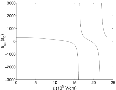
FIG. 1.: $a_{\rm sc}$ v.s. ${\cal E}$ for ⁴¹K in electron spin triplet state.

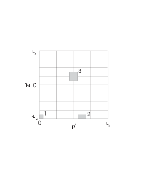
FIG. 2.: Computation of kernel

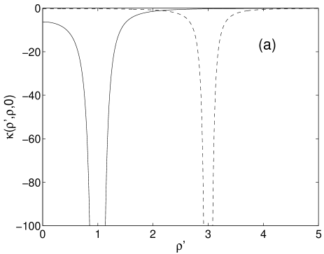
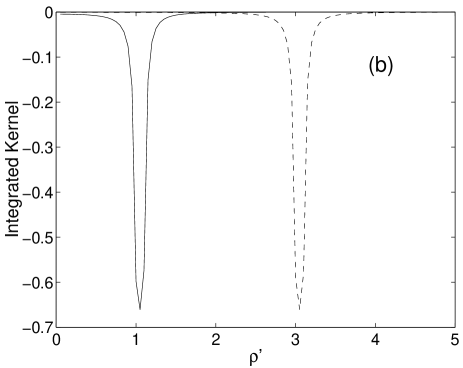
FIG. 3.: Typical behavior of ${\cal K}(\rho^{\prime},\rho,0)$ (a) and the corresponding integrated kernel over the wave function grid (b). The solid (dashed) lines are for $\rho=1.0$ (3.0).

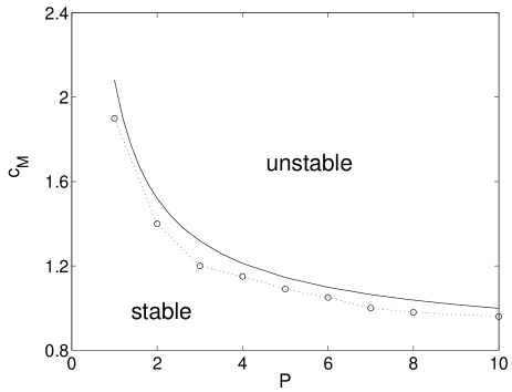
FIG. 4.: $c_{M}$ at the highest field value of condensate collapsing for $\lambda=1$. Numerically computed values are in circles connected by a dotted line. The solid line is from the variational calculation.

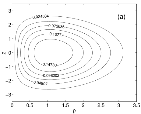
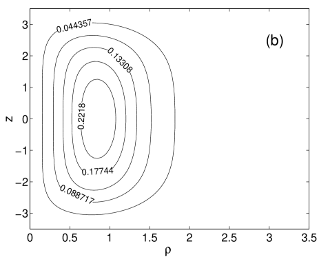
FIG. 5.: $n=1$ vortex state wave function with a) no external electric field; b) $c({\cal E})=2.0$. Other parameters are $P=10$ and $\lambda=1$.

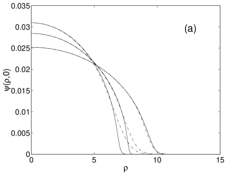
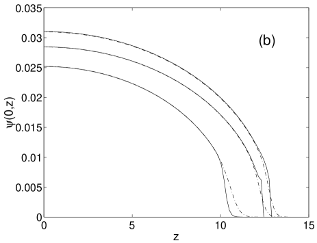
FIG. 6.: Ground state wave functions with (solid line) and without (dash-dotted line) TFA. $P=5000$, $\lambda=1$ and $c({\cal E})=0.7,0.6,0.2$ in descending order of wave function values at the origin.

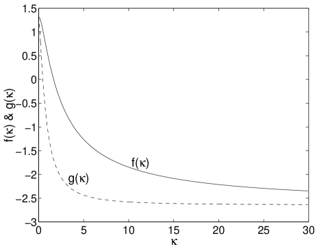
FIG. 7.: $f(\kappa)$,$g(\kappa)$

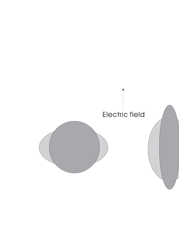
FIG. 8.: Condensates (pancake shaped in the left and cigar shaped to the right) always expands along the direction of an externally applied electric field and shrinks along the repulsive radial directions. Darker ellipses are for higher electric fields.

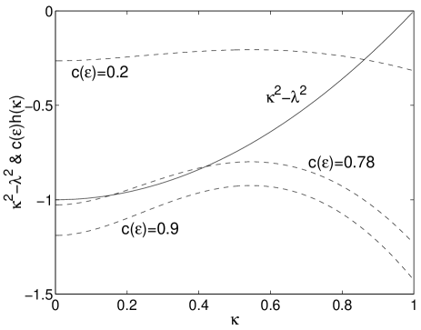
FIG. 9.: Graphic solutions of Eq. (67) for $\lambda=1$. Functions $\kappa^{2}-\lambda^{2}$ (solid line) and $c({\cal E})h(\kappa)$ (dashed line) for different values of $c({\cal E})$.

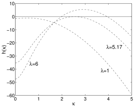
FIG. 10.: Function $h(\kappa)$ for different $\lambda$ value.

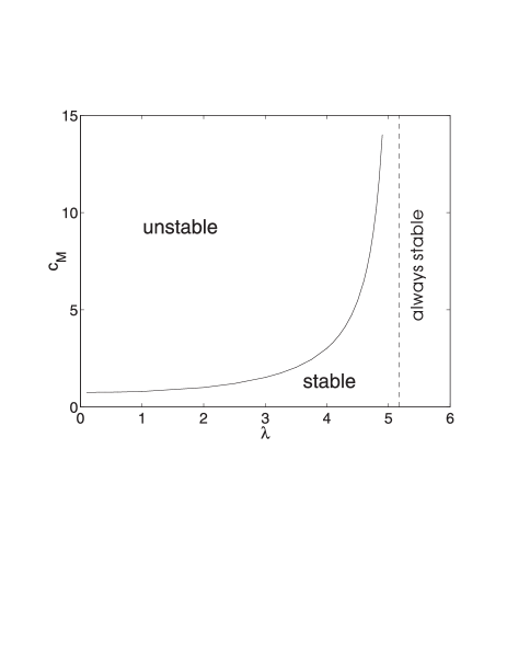
FIG. 11.: $c_{M}$ as a function of $\lambda$ with TFA.

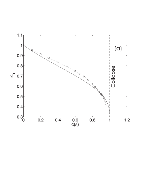
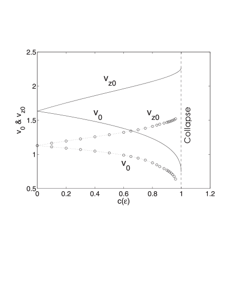
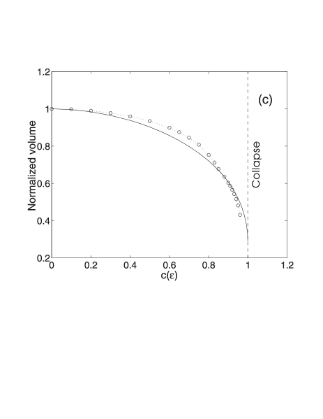
FIG. 12.: Field dependence of $\kappa_{0}$ (a), $v_{0}$, $v_{z0}$ (b) and normalize volume (c) of condensate for $P=10$, $\lambda=1$. Numerically computed results are in circles connected by dotted lines, the solid lines are from variational calculations.

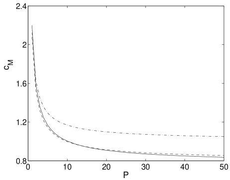
FIG. 13.: $c_{M}$ as a function of $P$, for $\lambda=0.5$ (solid), $1.0$ (dashed), and $2.0$ (dash-dotted line). As $P\rightarrow\infty$, $c_{M}$ goes to the value obtained under TFA.

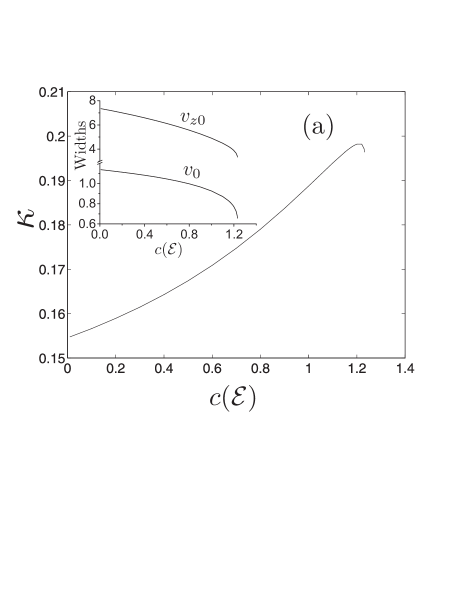
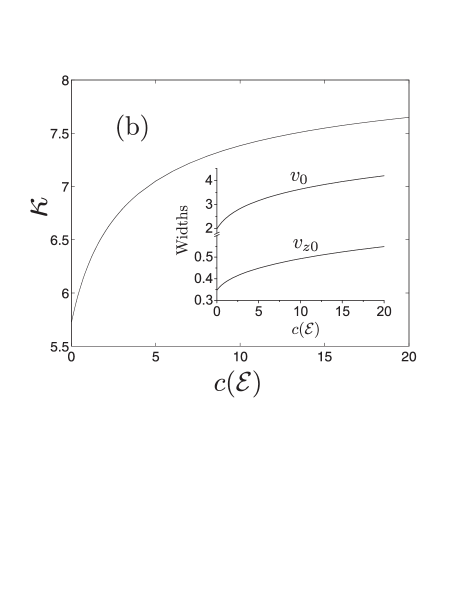
FIG. 14.: Field dependence of $\kappa_{0}$ and condensate widths (in insets) for $P=5$, $\lambda=0.1$ (a) and $\lambda=10$ (b). When $\lambda<\lambda_{c}$, the volume of condensate decreases with $c(\cal E)$. It increases with $c(\cal E)$ when $\lambda>\lambda_{c}$, causing condensate to be always stable.

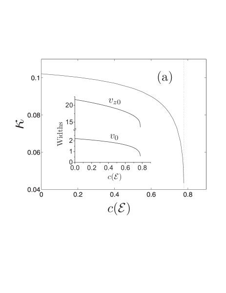
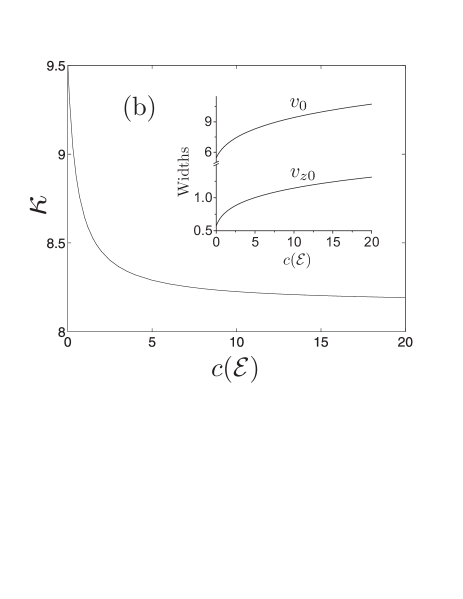
FIG. 15.: The same as in Fig. 14, but now for $P=500$.

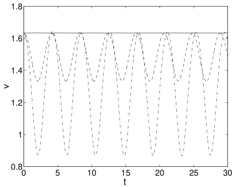
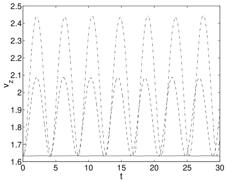
FIG. 16.: Evolution of condensate widths for $P=10$, $\lambda=1$, $v(0)=v_{z}(0)=1.63359$ at $c({\cal E})=0.0$ (solid line), $c({\cal E})=0.4$ (dashed line), and $c({\cal E})=0.8$ (dash-dotted line).

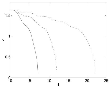
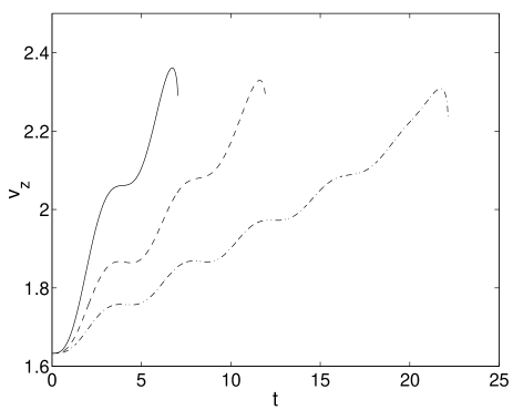
FIG. 17.: Evolution of condensate widths at $c({\cal E})=1.0$ ($>c_{M}=0.9989$), for electric field ramp-up time $T=5$ (solid line), $10$ (dashed line), and $20$ (dash-dotted lines). Other parameters are $P=10$, $\lambda=1$, and $v(0)=v_{z}(0)=1.63359$.

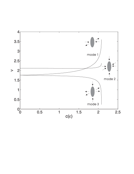
FIG. 18.: Electric field dependence of the shape oscillation frequencies. Other parameters are $P=1$ and $\lambda=1$.

REFERENCES

- [1] M. H. Anderson, J. R. Ensher, M. R. Matthews, C. E. Wieman, and E. A. Cornell, Science 269, 198 (1995).
- [2] K. B. Davis, M.-O. Mewes, M. R. Andrews, N. J. van Druten, D. S. Durfee, D. M. Kurn, and W. Ketterle, Phys. Rev. Lett. 75, 3969 (1995).
- [3] C. C. Bradley, C. A. Sackett, J. J. Tollett, and R. G. Hulet, Phys. Rev. Lett. 75, 1687 (1995); Erratum: ibid 79, 1170 (1997).
- [4] Extentive list of references exists at: http://amo.phy.gasou.edu/bec.html/bibliography.html .
- [5] E. P. Gross, Nuovo Cimento 20, 454 (1961); L. Pitaevskii, Sov. Phys. JETP 13, 451 (1961).
- [6] F. Dalfovo, S. Giorgini, L.P.Pitaevskii, S.Stringari, Rev. Mod. Phys. 71, 463 (1999).
- [7] Y. Castin and R. Dum, Phys. Rev. Lett. 77, 5315 (1996).
- [8] Yu. Kagan, E. L. Surkov, and G. V. Shlyapnikov, Phys. Rev. A 54, R1753 (1996).
- [9] Kerson Huang and C. N. Yang, Phys. Rev. 105, 767 (1957).
- [10] M. Naraschewski and R. J. Glauber, Phys. Rev. A 59, 4595 (1999).
- [11] B. Esry and C. Greene, Phys. Rev. A 60, 1451 (1999).
- [12] P. O. Fedichev et al., Phys. Rev. Lett. 77, 2913 (1996); J. L. Bohn and P. S. Julienne, Phys. Rev. A 56, 1486 (1997).
- [13] A. J. Moerdijk, B. J. Verhaar, and T. M. Nagtegaal, Phys. Rev. A 53, 4343 (1996).
- [14] E. Tiesinga, A. J. Moerdijk, B. J. Verhaar, and H. T. C. Stoof, Phys. Rev. A 46, R1167 (1992).
- [15] S. Inouye, M. R. Andrews, J. Stenger, H. -J. Miesner, D. M. Stamper-Kurn, and W. Ketterle, Nature (London) 392, 151 (1998); Ph. Courteille, R. S. Freecand, D. J. Heinzen, F. A. van Abeelen, and B. J. Verhaar, Phys. Rev. Lett. 81, 69 (1998); S. L. Cornish, N. R. Claussen, J. L. Roberts, E. A. Cornell, C. E. Wieman, (cond-mat/0004290).
- [16] J. L. Roberts, N. R. Claussen, J. P. Burke, Jr., C. H. Greene, E. A. Cornell, and C. E. Wieman, Phys. Rev. Lett. 81, 5109 (1998); Vladan Vuletic, A. J. Kerman, C. Chin, and S. Chu, ibid 82, 1406 (1999).
- [17] M. Marinescu and L. You, Phys. Rev. Lett. 81, 4596 (1998).
- [18] A. J. Leggett, Rev. Mod. Phys. 47, 331 (1975).
- [19] S. H. Pan, E. W. Hudson, K. M. Lang, H. Eisaki, S. Uchida, and J. C. Davis, Nature 403, 746 (2000).
- [20] P. A. Ruprecht, M. J. Holland, K. Burnett, and Mark Edwards, Phys. Rev. A 51, 4704 (1995).
- [21] C. C. Bradley, C. A. Sackett and R. G. Hulet, Phys. Rev. Lett. 78, 985 (1997).
- [22] M. Lewenstein and L. You, Phys. Rev. A 53, 909 (1996).
- [23] A. Parola, L. Salasnich, L. Reatto, Phys. Rev. A 57, R3180 (1998); L. Salasnich, ibid 61, 015601 (2000); V. M. Perez-Garcia, V. V. Konotop, J. J. Garcia-Ripoll, (cond-mat/9912301).
- [24] S. Yi and L. You, Phys. Rev. A 61, 041604(R) (2000).
- [25] K. Goral, K. Rzaewski, and Tilman Pfau, Phys. Rev. A 61, 051601(R) (2000).
- [26] L. Santos, G. V. Shlyapnikov, P. Zoller, and M. Lewenstein, (cond-mat/0005009)
- [27] J. D. Weinstein, R. deCarvalho, T. Guillet, B. Friedrich, J. M. Doyle, Nature 395, 148 (1998).
- [28] J. T. Bahns, P. L. Gould, and W. C. Stwalley, Adv. Atom Mol. and Opt. Phys. 42, 171 (2000); and extensive references therein.
- [29] V. Galitskii, Sov. Phys. JETP 34, 104 (1958) [Zh. Eksp. Teor. Fiz. 34, 151 (1958)].
- [30] S. T. Beliaev, Sov. Phys. JETP 7, 289 (1958) [Zh. Eksp. Teor. Fiz. 34, 417 (1958)]; N. M. Hugenholtz and D. Pines, Phys. Rev. 116, 489 (1959).
- [31] K. A. Brueckner and K. Sawada, Phys. Rev. 106, 1117 (1957).
- [32] M. Marinescu and L. You, (unpublished).
- [33] M. R. Matthews, B. P. Anderson, P. C. Haljan, D. S. Hall, C. E. Wieman, and E. A. Cornell, Phys. Rev. Lett. 83, 2498 (1999).
- [34] K. W. Madison, F. Chevy, W. Wohlleben, and J. Dalibard, Phys. Rev. Lett. 84, 806 (2000).
- [35] C. Raman, M. Kohl, R. Onofrio, D. S. Durfee, C. E. Kuklewicz, Z. Hadzibabic, and W. Ketterle, Phys. Rev. Lett. 83, 2502 (1999).
- [36] L. P. Pitaevskii, Phys. Lett. A 221, 14 (1996).
- [37] G. Baym and C. J. Pethick, Phys. Rev. Lett. 76, 6 (1996).
- [38] Victor M. Perez-Garcia, H. Michinel, J. I. Cirac, M. Lewenstein, and P. Zoller Phys. Rev. Lett. 77, 5320 (1996); Phys. Rev. A 56, 1424 (1997)
- [39] U. Al Khawaja and H. T. C. Stoof, (cond-mat/0003517).
- [40] D. S. Jin, M. R. Matthews, J. R. Ensher, C. E. Wieman, and E. A. Cornell, Phys. Rev. Lett. 78, 764 (1997).
- [41] P. Ring and P. Schuck, The Nuclear Many-Body Problem, p. 172, (Springer-Verlag, New York, 1980).
- [42] H. L. Bethlem, G. Berden, and G. Meijer, Phys. Rev. Lett. 83, 1558 (1999).
- [43] H. Gould, Phys. Rev. A 14, 922 (1976).
- [44] R. Marrus, E. C. Wang, and J. Yellin, Phys. Rev. 177, 122 (1969).
- [45] J. A. Maddi, T. P. Dinneen, and H. Gould, Phys. Rev. A 60, 3882 (1999).
- [46] M. Dörr, R. M. Potvliege, and R. Shakeshaft, Phys. Rev. Lett. 64, 2003 (1990).