[

Gravity-driven Dense Granular Flows

Abstract

We report and analyze the results of numerical studies of dense granular flows in two and three dimensions, using both linear damped springs and Hertzian force laws between particles. Chute flow generically produces a constant density profile that satisfies scaling relations suggestive of a Bagnold grain inertia regime. The type of force law has little impact on the behavior of the system. Bulk and surface flows differ in their failure criteria and flow rheology, as evidenced by the change in principal stress directions near the surface. Surface-only flows are not observed in this geometry.

]

Understanding the behavior of granular materials has been a great challenge to scientists[2, 3] and engineers[4, 5]. One major hurdle has been the lack of a formal connection between the complicated but relatively well-understood world of contact mechanics[6], which describes the nature and dynamics of intergranular interactions, and empirical continuum models that describe the macroscopic behavior of the system.

We aim to isolate the essential features of granular flow, unencumbered by complicated boundary effects. To this end, we perform simulations of granular dynamics in a simple geometry: gravity driven dense flow down an inclined plane, denoted henceforth as “chute flow”. Several remarkable features emerge:

(1) In steady-state, the packing fraction $\phi$ remains constant as a function of depth, beyond a dilatant surface region a few layers thick (Fig. 1.) The compacting influence of increasing stress due to the weight of grains overhead is balanced by increasing velocity fluctuations towards the bottom of the assembly.

(2) Unlike Couette flows, the entire assembly is in motion and surface-only flows are not observed.

(3) Components of the stress tensor and the square of the strain rate grow linearly with depth, indicative of Bagnold grain-inertia behavior[7].

(4) Normal stresses differ from each other[8] in a systematic way (Fig. 2), which we do not fully understand.

We report results of large scale molecular dynamics simulations of chute flow in two and three dimensions (2D and 3D), with interparticle interactions betweeen the (monodisperse) spheres modeled using both damped linear springs and Mindlin-Hertz contact forces, with static friction. Detailed results of the simulations will be presented elsewhere[9]. The main obstacle for experiments and simulations so far has been the difficulty of reaching and maintaining steady state. Previous simulations[10] employed very few particles or did not reach steady state[11]. All of these simulations were in 2D with the exception of Walton[10]. Experiments on chute flow[12, 13] did not involve deep assemblies. Different effects of flow were also studied in simulation, such as size segregation[14].

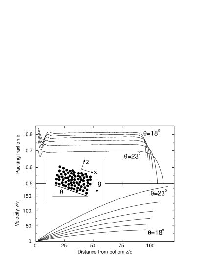
FIG. 1.: Density and velocity profiles as a function of height from the bottom of the assemblies for 2D (top) and 3D (bottom) simulations. Inset shows a schematic of the geometry. Results are for $10\,000$ particles in 2D and $8\,000$ in 3D. The characteristic velocity $v_{0}=\sqrt{gd}$.

FIG. 2.: Tilt dependence of the packing fraction (top) and the normal stress anomaly $(\sigma_{xx}-\sigma_{zz})/\sigma_{zz}$ (bottom) below the transitional surface layer. The dashed lines are fits to the forms Eq. (8 -9). The solid lines are guides to the eye.

The 3D simulation cells contain spheres of diameter $d$ and mass $m$, supported by a fixed bottom on the $x-y$ plane. The bottom wall is constructed from a cross-section of a random close packing of identical spheres, providing a rough surface. Periodic boundary conditions are imposed along $x$ and $y$ directions. 2D simulations follow the same procedure, except that particles are restricted to the $x-z$ plane and the bottom consists of a regular array of particles of diameter $2d$. In both cases, there is no slip observed at the bottom. (There is some slip in 2D with a regular array of particles of diameter $d$ at the bottom.) The gravity vector g is rotated by the tilt angle $\theta$ away from the $(-\hat{z})$ direction in the $x-z$ plane, so that the free surface is normal to the $\hat{z}$ axis. In 3D, most of our results are for $8\,000$ particle systems with a simulation cell of size $L_{x}=18.6d$ and $L_{y}=9.3d$, resulting in an assembly roughly 40 particles deep at rest. In 2D, $L_{x}=100d$ and the number of particles varied from a few hundred to $20\,000$. In this Letter, we present results for $N=10\,000$, with a depth of about 100 particles.

We use the contact force model of Cundall and Strack[15]. Static friction is implemented by keeping track of the elastic shear displacement throughout the lifetime of a contact. For two contacting particles at positions r₁ and r₂, with velocities v_1,2 and angular velocities $\mbox{\boldmath{$\omega$}}_{1,2}$, the force on particle 1 is computed as follows: The normal compression $\delta$, normal velocity ${\bf v}_{n}$, relative surface velocity ${\bf v}_{t}$, and the rate of change of the elastic tangential displacement ${\bf u}_{t}$, set to 0 at the initiation of a contact, are given by

$$\delta = d-||{\bf r}_{12}||,$$ (1)

$${\bf v}_{n} = ({\bf v}_{12}\cdot{\hat{r}}_{12}){\hat{r}}_{12},$$ (2)

$${\bf v}_{t} = {\bf v}_{12}-{\bf v}_{n}-(\mbox{\boldmath{$\omega$}}_{1}+\mbox{\boldmath{$\omega$}}_{2})\times{\bf r}_{12}/2,$$ (3)

$$\frac{d{\bf u}_{t}}{dt} = {\bf v}_{t}-\frac{({\bf u}_{t}\cdot{\bf v}_{12}){\bf r}_{12}}{||{\bf r}_{12}||^{2}},$$ (4)

where ${\bf r}_{12}={\bf r}_{1}-{\bf r}_{2}$, ${\hat{r}}_{12}={\bf r}_{12}/||{\bf r}_{12}||$, and ${\bf v}_{12}={\bf v}_{1}-{\bf v}_{2}$. The second term in Eq.(4) arises from the rigid body rotation around the contact point and assures that ${\bf u}_{t}$ always remains in the local tangent plane of contact. Normal and tangential forces acting on particle 1 are given by

$${\bf F}_{n} = k_{n}f(\delta/d)\left(\delta{\hat{r}}_{12}-\tau_{n}{\bf v}_{n}\right),$$ (5)

$${\bf F}_{t} = k_{s}f(\delta/d)\left(-{\bf u}_{t}-\tau_{s}{\bf v}_{t}\right),$$ (6)

where $k_{n,s}$ and $\tau_{n,s}$ are elastic constants and viscoelastic relaxation times respectively; $f(x)=1$ for damped linear springs or $f(x)=\sqrt{x}$ for Hertzian contacts between spheres. A local Coulomb yield criterion, $F_{t}<\mu F_{n}$, is satisfied by truncating the magnitude of ${\rm\bf u}_{t}$ as necessary. Thus, the contact surfaces are treated as “stuck” while $F_{t}<\mu F_{n}$, and slipping while the yield criterion is satisfied. This “proportional loading” approximation[16] is a simplification of the much more complicated and hysteretic behavior of real contacts[17]. The force on particle 2 is determined from Newton’s third law. Each particle is also subject to a body force

$${\bf F}_{\rm body}=mg(-{\hat{z}}\cos\theta+{\hat{x}}\sin\theta).$$ (7)

All results are given in terms of non-dimensionalized quantities: Distances, times, velocities, forces, elastic constants and stresses are reported in units of $d$, $t_{0}\equiv\sqrt{d/g}$, $v_{0}\equiv\sqrt{gd}$, $F_{0}\equiv mg$, $k_{0}\equiv mg/d$ and $\sigma_{0}\equiv mg/d^{2}$, respectively. The summary of parameters used in the simulations are shown in Table I. In these units, the correct elastic constant for glass spheres with $d=100\mu m$ would have been $k_{n}^{\rm glass}/k_{0}\approx 3\times 10^{10}$, which would have prohibited a large-scale simulation. We use $k_{n}/k_{0}=2\times 10^{5}$, while controlling the coefficient of restitution for binary collisions through $\tau_{n}$, assuming that we remain sufficiently close to the $k_{n}\to\infty$ limit of small deformations. Simulations for $k_{n}/k_{0}=2\times 10^{4}$ and $2\times 10^{6}$ in 2D gave essentially the same results, supporting this assumption. For Hertzian contacts, the ratio $k_{s}/k_{n}$ depends on the Poisson ratio of the material[17], and is about $2/3$ for most materials. We use the value $k_{s}/k_{n}=2/7$, since this makes the period of normal and shear contact oscillations equal to each other in the damped linear springs case[18]. The collisional dynamics are not very sensitive to the precise value of this ratio.

Dimen-	Force	$k_{n}/k_{0}$	$\tau_{n}/t_{0}$	$k_{s}/k_{n}$	$\tau_{s}/\tau_{n}$	$\mu$
sion	Law
2D	Linear	$2\times 10^{5}$	$8.375\times 10^{-5}$	2/7	0	0.5
3D	Hertzian	$2\times 10^{5}$	$1.25\times 10^{-4}$	2/7	0	0.5

TABLE I.: Simulation parameters for results shown. The normal coefficient of restitution for 2D simulations is 0.92; it is a function of collision velocity for Hertzian contacts in 3D simulations.

The equations of motion for the translational and rotational degrees of freedom were integrated with either a third-order Gear predictor-corrector or velocity-Verlet scheme with a time step $\delta t=1\times 10^{-4}$. Typically it was necessary to run between 5 and $20\times 10^{6}~{}\delta t$ to reach steady state, particularly when starting from a non-flowing state. All coarse grained quantities have been averaged both temporally (typically 2 to $8\times 10^{6}~{}\delta t)$ and spatially over slices of constant $z$.

The main characteristics of all the flows are: (i) The existence of an “angle of repose” $\theta_{r}$, such that granular flows can not be sustained for $\theta<\theta_{r}$, (ii) a steady-state flow with a packing fraction independent of depth for $\theta_{r}<\theta<\theta_{\rm max}$, and (iii) for $\theta>\theta_{\rm max}$, development of a shear thinning layer at the bottom of the assembly that results in lift-off and unstable acceleration of the entire assembly. For very thin assemblies, less than about $20$ layers, the value of $\theta_{r}$ depends on their depth, in agreement with experiment[13]. Here we consider only deep assemblies where the value of $\theta_{r}$ is independent of depth, and focus our attention on region (ii). As seen in Fig. 1, the packing fraction $\phi$ remains constant as a function of depth, away from the free surface and the bottom wall. Its value is shown as a function of $\theta$ in Fig. 2. Results in 2D for systems of size $5\,000$ and $20\,000$ demonstrate that the thicknesses of the boundary layers at the bottom and top are independent of the height of the assembly. The data suggest an approximate tilt dependence for $\phi$ of the form

$$\phi_{2D}(\theta) \approx \phi_{2D}^{\rm max}-c_{2D}(\theta-\theta_{r,2D})^{2},$$ (8)

$$\phi_{3D}(\theta) \approx \phi_{3D}^{\rm max}-c_{3D}(\theta-\theta_{r,3D}),$$ (9)

where $\phi_{2D}^{\rm max}=0.810(5)$ and $\phi_{3D}^{\rm max}=0.595(5)$.

In 2D, upon lowering the tilt angle below $\theta_{r}$, we observe a compaction to a polycrystalline triangular lattice with $\phi_{2D}\approx 0.9$. This causes considerable hysteresis in 2D simulations as $\theta$ is subsequently increased beyond $\theta_{r}$: There is no flow until a maximum angle of stability is exceeded. Initial failure always occurs at the bottom, followed by movement of a dilation front towards the top. Once the system reaches steady state, $\theta$ can be reduced and the system continues to flow while $\theta>\theta_{r}$. On the other hand, in 3D there is no jump in $\phi$ as the system comes to a stop, and no detectable hysteresis as the system is stopped and restarted by varying $\theta$. Thus, Mohr-Coulomb analysis of the stress tensor[4] can be used to relate the flow rheology near $\theta_{r}$ to the Coulomb failure criterion as follows: The Mohr circle is the set of normal and shear stresses ($\sigma$ and $\tau$, see inset in Fig. 3) associated with all possible shear planes. The points $A$ and $B$ at coordinates $(\sigma_{zz},\sigma_{xz})$ and $(\sigma_{xx},-\sigma_{xz})$ in the $(\sigma,\tau)$ plane form a diameter of the circle. At a given tilt angle, $\sigma_{zz}$ and $\sigma_{xz}$ are determined by force balance, which pins down the location of point $A$ ($\sigma_{xz}/\sigma_{zz}=\tan\theta$; see Fig. 3, inset.)

FIG. 3.: Left: The gap angle $\delta\theta$ (defined pictorially in the inset) as a function of height for $\theta=20^{\circ}$ (circles), $22^{\circ}$ (squares), $24^{\circ}$ (diamonds), and $26^{\circ}$ (triangles). The lines are fits that decay exponentially from $\delta\theta^{\rm surf}$ to $\delta\theta^{\rm bulk}$ with a typical decay length of 1.5 to $2.5d$, inidcating a surface layer about $5d$ to $8d$ thick. Right: Although $\delta\theta^{\rm surf}$ vanishes at $\theta=\theta_{r}$, $\delta\theta^{\rm bulk}$ remains finite, suggesting that the initiation of flow is controlled by the surface rather than the bulk (see text.)

However, $\sigma_{xx}$, thus the location of point $B$, remains indeterminate from these considerations. The “gap angle” $\delta\theta\equiv\theta_{MC}-\theta$ is a measure of the difference between $\tau/\sigma$ along the slip plane parallel to the surface ($=\tan\theta$) and the largest value of $\tau/\sigma$ experienced by the system (equal to the slope $\tan\theta_{MC}$ of the line that passes through the origin and that is tangent to the Mohr circle.) For an ideal Coulomb material with a uniform yield criterion, $\delta\theta=0$ at $\theta=\theta_{r}$, when the static system is at incipient yield. The behavior of $\delta\theta$ as a function of depth at different tilt angles, as shown in Figure 3, reveal that: (i) $\delta\theta$ becomes independent of depth below a transitional surface layer about $5d$ to $8d$ in thickness, (ii) the gap angle remains finite at the bottom and in the bulk but vanishes at the top surface when $\theta=\theta_{r}$. It thus seems that although the bulk of the system has the intrinsic capability to withstand slightly larger tilt angles, the destabilization of the surface at $\theta=\theta_{r}$ is ultimately responsible for the failure and initiation of flow in the entire system. Note that the transitional surface layer is not directly related to the dilatant layer; it is much thicker near $\theta=\theta_{r}$ and penetrates well into the region of constant density. Interestingly, in 2D the gap angle at $\theta_{r}$ is actually larger at the surface compared to the bulk, and both gap angles remain finite. However, the presence of hysteresis precludes us from applying the Mohr-Coulomb analysis in 2D.

A feature that distinguishes granular flows from Newtonian fluid flows is that normal stresses, i.e., diagonal terms in the stress tensor, are in general not equal to each other[8]. Although $\sigma_{xx}\approx\sigma_{zz}$ in our simulations, we observe small but systematic deviations, which are depicted in Fig. 2 by plotting the normal stress anomaly in the bulk, $(\sigma_{xx}-\sigma_{zz})/\sigma_{zz}$, as a function of tilt angle. These deviations are likely to be due to a constitutive equation of the flow rheology which we have not yet been able to determine. In addition, in all 3D runs, $\sigma_{yy}$ is smaller than the other normal stresses by $10-15\%$, suggesting that consolidation and compaction normal to the shear plane is poorer.

Another question of particular interest is the relationship between the stresses and strain rate. Shear stress $\sigma_{xz}$ is a linear function of strain rate $\dot{\gamma}\equiv\partial v_{x}/\partial z$ for viscous fluids, and quadratic in $\dot{\gamma}$ for granular systems in the Bagnold grain-inertia regime. The latter result is rather general: When typical stresses on grains are large compared to the weight of individual particles but not large enough to significantly distort the spheres $(1\ll\sigma/\sigma_{0}\ll k_{n}/k_{0})$, the only relevant time scale is $\dot{\gamma}^{-1}$, which forces $\sigma_{xz}\propto\dot{\gamma}^{2}$ simply by dimensional analysis. As an example, Fig. 4 shows the relationship between shear strain rate $\dot{\gamma}$ and shear stress $\sigma_{xz}$ for 2D and 3D cases. Below the transitional surface layer, and away from the bottom wall, both systems exhibit Bagnold scaling, indicated by the dashed lines in Fig. 4. Data for 2D suggest an offset of about $1.5\sigma_{0}$ in the stress, possibly due to corrections from the body force on individual spheres. Such an offset is not needed for an acceptable fit to the 3D data.

FIG. 4.: Strain rates plotted as a function of shear stress $\sigma_{xz}$ for 2D (top) and 3D (bottom) reveal Bagnold scaling (dashed lines) in the constant packing fraction regime away from the free surface and the bottom wall. For 2D, an offset of $1.5\sigma_{0}$ in the shear stress was needed for an acceptable fit.

In order to probe the sensitivity of the results to the exact form of the stiff elastic response, we have also performed runs in the 3D system with linear damped springs, keeping all other parameters fixed[9]. Remarkably, the packing fraction profiles and the normal stress anomaly remained virtually the same, and strain rate profiles were changed only by a global factor of about 1.35, suggesting that results are not too sensitive to the particular force scheme selected.

The lack of a regime with only surface flow is in contrast with experimental observations of avalanche flows in rotating drums[3]. Since periodic boundary conditions are used, our simulations correspond to an infinitely large system with finite depth and fixed surface tilt, and therefore constitutes a different system. Experiments on chute flows[8] also lack a regime of surface only flow; although this might be attributed to side-wall friction that necessitates higher tilt angles to initiate flow. Although there is no fundamental reason we can find that prohibits surface-only flows in this geometry, it appears that they are unlikely to occur in an assembly of monodisperse spheres.

DL is supported by the Israel Science Foundation under grant 211/97. Sandia is a multiprogram laboratory operated by Sandia Corporation, a Lockheed Martin Company, for the United States Department of Energy under Contract DE-AC04-94AL85000.

REFERENCES

- [1] E-mail address: mdertas@erenj.com.
- [2] C. A. Coulomb, Mem. de Math. de l’Acad. Royales des Science 7 343 (1776).
- [3] H. M. Jaeger, S. R. Nagel, and R. P. Behringer, Rev. Mod. Phys. 68, 1259 (1996).
- [4] R. M. Nedderman, Statics and Kinematics of Granular Materials (Cambridge University Press, Cambridge, England,1992).
- [5] R. L. Brown and J. C. Richards, Principles of Powder Mechanics (Pergamon Press, Oxford, England, 1970).
- [6] K. L. Johnson, Contact Mechanics (Cambridge University Press, New York, 1985).
- [7] R. A. Bagnold, Proc. Roy. Soc. London A 225, 49 (1954); ibid., 295, 219 (1966).
- [8] S. B. Savage, J. Fluid Mech. 92, 53 (1979).
- [9] L. Silbert et al., to be published.
- [10] O. R. Walton, Mech. Mater. 16, 239 (1993); X. M. Zheng and J. M. Hill, Powder Tech. 86, 219 (1996); O. Pouliquen and N. Renaut, J. Phys. II France 6, 923 (1996).
- [11] T. Pöschel, J. Phys. II France 3, 27 (1993).
- [12] T. Drake, J. Geophysical Res. 95, 8681 (1990).
- [13] O. Pouliquen, Phys. Fluids 11, 542 (1999).
- [14] D. Hirshfield and D. C. Rapaport, Phys. Rev. E 56, 2012 (1997).
- [15] P. A. Cundall and O. D. L. Strack, Geotechnique 29, 47 (1979).
- [16] T. C. Halsey and D. Ertaş, Phys. Rev. Lett. 83, 5007 (1999).
- [17] R. D. Mindlin and H. Deresiewicz, L. Appl. Mech. 20, 327 (1953).
- [18] J. Schäfer, S. Dippel and D. E. Wolf, J. Phys. I France 6, 5 (1996).