On the Effects of Changing the Boundary Conditions on the Ground State of Ising Spin Glasses

Abstract

We compute and analyze couples of ground states of $3D$ spin glass systems with the same quenched noise but periodic and anti-periodic boundary conditions for different lattice sizes. We discuss the possible different behaviors of the system, we analyze the average link overlap, the probability distribution of window overlaps (among ground states computed with different boundary conditions) and the spatial overlap and link overlap correlation functions. We establish that the picture based on Replica Symmetry Breaking correctly describes the behavior of $3D$ Spin Glasses.

I Introduction

Understanding the structure of the states of three dimensional ($3D$) Ising spin glasses at finite temperature is a very interesting problem. Long time ago a mean field theory for spin glasses has been constructed and successfully compared with the numerical properties of a long range model, the Sherrington-Kirkpatrick model, where mean field theory is exact by definition [1].

In the mean field approach one finds that the free energy landscape is strongly corrugated, and it is characterized by the presence of many local minima, which correspond to spin configurations very different one from the other. There are many low free energy local minima which have a total free energy which differs from the ground state free energy of an amount which is of order $1$; these minima contribute to the probability distribution of the spins also for arbitrary large volumes. In some sense one can say that in the infinite volume there are many equilibrium states (for a better qualification of the terminology see [2]): these states are locally different one from the other. For historical reasons this picture goes under the name of Replica Symmetry Breaking (RSB).

Since analytic progress on finite dimensional system is hard, the study of $3D$ systems has mainly been based on numerical simulations. Most of the numerical simulations have investigated systems of size up to $V\equiv L^{3}=16^{3}$ and temperature values greater or equal than half of the critical temperature ($T_{c}$): the results are in very good agreement with the RSB picture. Using the best techniques that are available to us today it is impossible to thermalize in a reasonable amount of time systems of this size at much lower temperature: because of that at today the very low temperature region cannot be explored using Monte Carlo simulations. On the other end a different class of algorithms exists which allow the determination of the ground state at zero temperature for systems of comparable size [3, 4, 5, 6]: it is clear that it would be very interesting to compare the results of the RSB approach with the numerical results at zero temperature.

We face however a difficulty: in the RSB approach one computes quantities at finite temperature in the infinite volume limit, while if we look first for the ground state in a finite volume and only later we send the volume to infinity we are exchanging the order of the two limits. One can assume in a tentative way that the two limits can be exchanged, in the sense that in the zero temperature limit the probability distributions of the free energies of different equilibrium states becomes the probability distributions of the local minima of the energy: this has been the point of view of the authors that have employed this technique in the last months, it is not incompatible with any of the findings obtained to date, and we will do the same in the following.

Of course at zero temperature the ground state (i.e. the global minimum of the energy) of a finite volume system with quenched random couplings selected under a continuous distribution is unique, so that interesting information can be extracted for example if we consider the effects of an external perturbation.

Different choices are possible. In a recent, very interesting paper, Palassini and Young [7] have shown that it is possible to get useful information about the nature of the low $T$ phase of $3D$ Ising spin glasses with Gaussian distributed couplings by studying the behavior of the ground state after changing the boundary conditions of an $L^{3}$ lattice system from periodic ($PBC$) to anti-periodic ($ABC$). They analyze ground states ($GS$) obtained with the same realization of the quenched disorder and different boundary conditions (or with disorder realizations that differ only in some locations) for $L\leq 10$. In this paper we perform a more detailed analysis of the same systems by considering a larger set of observables. Here we use a modified genetic algorithm which is more efficient than the original algorithm and that will be described in details elsewhere [8]. This modified algorithm has allowed us to study larger systems ($L\leq 14$) than in former work. We arrive at the conclusion that the whole set of data strongly suggests that the picture based on Replica Symmetry Breaking is correct in describing the behavior of $3D$ Spin Glasses.

II Some Theoretical Considerations

A Four Possibilities

As we have already discussed in the introduction we consider a $3D$ Ising spin glass with quenched couplings assigned under a Gaussian probability distribution with zero expectation value, and we study the behavior of the ground state after changing the boundary conditions ($BC$) of a simple cubic lattice system of size $V=L^{3}$ from periodic ($P$) to anti-periodic ($AP$). When we do such a change the ground state is usually modified and in the new ground state some spins are reversed. Let us call $\sigma(i)$ and $\tau(i)$ the spins in the ground states with periodic and anti-periodic boundary conditions respectively. The local overlap on site $i$ is defined as

$$q(i)\equiv\sigma(i)\ \tau(i)\ .$$ (1)

The link overlap is defined on the links and it is given by

$$q_{l}(i,\mu)\equiv q(i)\ q(i+\mu)\ ,$$ (2)

where $\mu$ is the direction of the link, that can take $D$ positive and $D$ negative values. If two spin configurations differ by a global reverse of the spins their link overlap is identically equal to one (while their overlap is equal to $-1$). We will consider in the following the case where we flip the boundary conditions in the direction $x$, while we leave them unchanged in directions $y$ and $z$.

In a first approximation (neglecting the points at the boundaries, see next subsection) we can define the interface among the flipped and the non flipped region as the sets of link where $q_{l}(i,\mu)=-1$. We are interested in finding out the geometrical properties of this interface in the infinite volume limit. Of course the probability of finding the interface on a random link is given by

$$\rho\equiv\frac{1}{2}(1-q_{l})\ ,$$ (3)

where $q_{l}$ is the disorder expectation value of $q_{l}(i,\mu)$, averaged over sites $i$ and directions $\mu$.

Here we discuss a few possible situations:

1. The interface is confined in a region of width $L^{z}$ (with $z<1$): inside this region the interface may have overhangs. The interface density goes to zero as $L^{-\alpha}$ with $\alpha\geq 1-z$. This is what happens in ferromagnetic models, both with ordered and disordered Hamiltonians, where $\alpha=1$, al least in the ordered case. We will see immediately that this possibility is completely excluded by the data.

2. The wandering exponent $z$ is equal to one and the interface density goes to zero as $L^{-\alpha}$. We also assume than in the large volume limit the interface is a fractal object with fractal dimension $D_{s}=D-\alpha$ (where the space dimension $D$ is equal to 3). More precisely we assume that if we define a continuous coordinate (in the interval $[0-1]$) as $\frac{i}{L}$, in the infinite volume limit the interface becomes a fractal object defined on the continuum characterized by a fractal dimension $D_{s}$. In other words we are assuming that the interface is not a multi-fractal (i.e. that it can be characterized by a single fractal dimensions as usually happens for fractal objects one defines on a lattice in statistical mechanics), and so the relation $D_{s}=D-\alpha$ is consistent.

3. The exponent $\alpha$ is equal to zero and the density $\rho$ goes to a non zero value (i.e. $q_{l}$ does not go to $1$ in the large volume limit). Here the interface is space filling and in the above described continuum limit, the interface is a dense set of measure $1$. We expect that the probability that the interface does not intersect a region $\cal R$, whose size is proportional to the system size, goes to zero when the volume goes to infinity. On the contrary in the previous case such a probability would be a non trivial function of $\cal R$. As we shall see later, this possibility is the one realized in the case of RSB.

4. There is a last possibility, which is unusual, and we mention for completeness (although its description will take a disproportionate amount of space): this is when the wandering exponent $z$ is equal to one and $\alpha$ is greater than zero, but in continuum limit the interface does not become a fractal object of dimension $D_{s}=D-\alpha$, but it becomes a dense set. This happens for example if we consider a set of parallel planes at distance proportional to $L^{\alpha}$ or a set of isolated points at distance $L^{\frac{\alpha}{D}}$. In both cases the density goes to zero as $L^{-\alpha}$, but the resulting object is not a fractal in the infinite volume limit. A similar case happens in three dimensions if we take a random walk of length ${\cal L}=L^{3-\alpha}$ with $\alpha<1$. The system is a fractal of dimension $D_{s}$ up to a distance $\xi(L)$, while it looks homogeneous at larger distances.

   In this case the density-density correlation function will scale as

   $$C(x,L)\equiv\left.\overline{\rho(x)\rho(0)}\right|_{L}\propto L^{-\alpha}x^{-C_{s}}$$ (4)

   in the region $1\ll x\ll\xi(L)$, where $C_{s}=D-D_{s}$ is the co-dimension of the fractal (the underlying random walk in our case). We will denote by the upper bar the average over the quenched disorder. On the contrary in the region $\xi(L)\ll x$ the correlation function will scale as

   $$C(x,L)\propto L^{-2\alpha}\ .$$ (5)

   The condition that at large distances the term in equation (5) dominates over the one in equation (4) implies that $C_{s}>\alpha$. Moreover the two formulas must be consistent in the crossover region where $x\approx\xi(L)$. Imposing this condition one finds that $L^{-\alpha}\xi(L)^{-C_{s}}\propto L^{-2\alpha}$ and therefore we obtain that

   $$\xi(L)\propto L^{\omega}\ ,\ \ \ \omega={\alpha\over C_{s}}<1\ .$$ (6)

   This case is anomalous in the sense that usual scaling is not valid and there is a crossover length which increases as a fractional power of the side of the system. The usual scaling law (valid in the region $x=O(L)$)

   $$C(x,L)=L^{-2\alpha}f(xL^{-1})$$ (7)

   is not satisfied and it is replaced by the unusual relation

   $$C(x,L)=L^{-\alpha-C_{s}}f(xL^{-1})+AL^{-2\alpha}g(xL^{-1})\ .$$ (8)

   Only in the case $\alpha=0$ we are in a familiar situation: in this case the crossover length $\xi$ does not diverge for large $L$ and we recover the third case of our list.

B The Effect of Changing Boundaries

In the replica approach one finds that at zero temperature there are many different local minima of the Hamiltonian such that even in the limit where $L$ goes to infinity the difference among the energy of the ground state and the energy of such minima is of order $1$. It is crucial that the among these minima there are some whose site overlap $q$ and link overlap $q_{l}$ with the ground state remains different from $1$ in large volume limit. It is also important to assume that for large volumes there exists a function $f$ such that $q_{l}=f(q^{2})$, in other words that for fixed overlap $q$ the link overlap $q_{l}$ does not fluctuate when the volume goes to infinity.

When in a $3D$ spin glass the boundary conditions in the $x$ direction are flipped from positive to negative it is known that the total energy changes by an amount $\Delta E$, which increases as a power of $L$. In a ferromagnet, where the ground state is unique, the ground state obtained under anti-periodic condition would be locally similar to the ground state obtained under periodic boundary conditions. In other words in any region of side $M$, if the region does not intersect the interface, which is just a flat surface, the ground state spin configuration obtained under anti-periodic boundary conditions will be equal (or equal to the reverse) to the ground state obtained under periodic boundary conditions.

A similar conclusion holds in the case of a spin glass behaving according to the predictions of the droplet model [9], where the boundary may be a corrugated surface: in this case we expect that the link overlap among the ground states obtained with $PBC$ and $ABC$ tends to one in the infinite volume limit. On the contrary in the case of a RSB like behavior the ground state obtained under $ABC$ can be locally similar to one of the low energy excited states: in this case the link overlap among the two ground states can tend to a value different from one as $L\to\infty$.

That an excited state may be selected as new ground state when changing the boundary conditions is strongly suggested by the fact that the energy difference among ground states obtained with periodic and anti-periodic boundary conditions increases with $L$, while the difference among the ground state energy and the excited state energy at fixed boundary conditions remains fixed.

The nature of the excited state that is selected when we change the boundary conditions cannot easily derived using simple arguments. It is reasonable to assume that in three dimensions, where $\Delta E$ which increases as a power of $L$, the new ground state will be as different as possible from the old ground state: one expects the overlap $q$ among the two ground states to vanish in this limit.

The interest in changing the boundary conditions is also due to the fact that this is also a convenient method to to study the properties of the excited states. Other methods can be used to clarify similar questions, but we will not use them here.

C Gauge Invariance

In order to change the boundary conditions in the $x$ direction we can change the sign of all the couplings connecting the plane $x=x_{0}$ with the plane $x=x_{0}+1$. The choice of $x_{0}$ does not matter: the ground state energy does not depend on $x_{0}$, and the ground state obtained after a different choice of the reversed plane (e.g. $x=x_{1}$) can be obtained starting from the ground state where anti-periodic boundary conditions have been enforced at $x_{0}$, by flipping all the spins in the interval $x_{0}<x\leq x_{1}$.

In other words going from periodic to anti-periodic boundary conditions is a global change that locally is not visible. At this end it is convenient to define quantities which are gauge invariant, in the sense that they do not change when the plane where the anti-periodic boundary conditions are imposed.

Let us consider a very simple example: the correct definition of $q_{l}(i,+\hat{x})$ is

$$q_{l}(i,+\hat{x}) \equiv q(i)\ q(i+\hat{x})\ \ \ \ \mbox{for}\ \ \ x\neq x_{0},$$ (9)

$$q_{l}(i,+\hat{x}) \equiv -q(i)\ q(i+\hat{x})\ \ \ \ \mbox{for}\ \ \ x=x_{0}\ ,$$ (10)

where $x$ is the first component of the three dimensional vector $i$.

A more complex case is the definition of the window overlap [10] in a box of side $M$ which intersects the plane $x=x_{0}$. Here the overlap $q_{M}$ can be defined as

$$\sum_{i\in{\cal A}}q(i)-\sum_{i\in{\cal B}}q(i)$$ (11)

where $\cal A$ and $\cal B$ are the set of points of the box which are respectively on the right and on the left of the plane $x=x_{0}$.

The advantage of this prescription (which can be easily generalized to more complex situations) is that in absence of a magnetic field nothing depends on the actual position of the plane where the boundary conditions are enforced: the fact that the reversal of the spins is imposed at a given value of $x$ is immaterial. The presence of this translational invariance is very effective from a practical point of view: the expectation value of $q_{l}$ does not depend on the point, so that data can be taken on the whole lattice. The possibility of doing measurements on the whole lattice and not only far from the point where the boundary conditions are changed reduces the statistical errors in a substantial way.

III A First Look to the Numerical Results

We have computed $16000$ couples of ground states on three dimensional lattices of linear size $L=4$, $73740$ for $L=6$, $8532$ for $L=8$, $2434$ for $L=10$, $910$ for $L=12$ and $670$ for $L=14$: for each sample of the quenched disorder (Gaussian couplings) we have computed the two ground states under periodic and anti-periodic boundary conditions, using a modified genetic algorithm which will be described elsewhere [8].

A The Average Link Overlap

The introduction of anti-periodic boundary conditions breaks the discrete rotational invariance of the simple cubic lattice, so that the expectation value of $q_{l}(i,\hat{x})$, i.e. of the link overlap in the $x$ direction, can be different from that of the link overlap in the other two directions. In the ferromagnetic case (without disorder) the change of the boundary conditions produces an interface in one of the $y-z$ planes. We will call perpendicular link overlap $q_{P}$ the expectation value of $q_{l}(i,\hat{x})$ averaged over the lattice sites, since it is perpendicular to the $y-z$ interface, while we will call transverse link overlap $q_{T}$ the average over sites of the quantity $\frac{1}{2}\left(q_{l}(i,\hat{y})+q_{l}(i,\hat{z})\right)$.

In the ferromagnetic case (without disorder) one finds that

$$1-q_{P}=\frac{1}{L},\ \ \ \ 1-q_{T}=0\ .$$ (12)

We show in figure (1) the numerical data for $1-q_{T}$ and $1-q_{P}$ in our $3D$ spin glass. It is clear that the difference $q_{T}-q_{P}$ goes to zero with $\frac{1}{L}$: it can be very well fitted as $aL^{-b}$ with $b\simeq 2.5$ and a normalized $\chi^{2}$ of order one.

It is also evident that $1-q_{P}$ is with a very good approximation a linear function of $L^{-1}$ in the same way it would be in the ferromagnetic case, with the difference that here the extrapolation in the $L\to\infty$ limit is clearly different from zero.

A closer look shows that $1-q_{P}$ is not exactly a linear function of $L^{-1}$, and it can be very well fitted (with a normalized $\chi^{2}$ of order one) as a second order polynomial in $L^{-1}$. The same polynomial fit works very well also for $1-q_{T}$. The two fits extrapolate to the same value (in the limit given by the statistical error). In the same picture we show also the data for $1-q_{P}-\frac{1}{L}$, i.e. the value we measure for $1-q_{P}$ in our spin glass minus its a priori lower bound, which coincides with the value in the ferromagnetic case, and we note it has a very weak dependence over $L$.

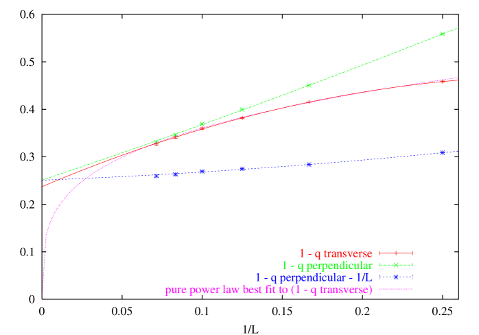
FIG. 1.: $1-q_{T}$, $1-q_{P}$ and $1-q_{P}-\frac{1}{L}$ versus $\frac{1}{L}$ for $L$ $=$ $4$, $6$, $8$, $10$, $12$, $14$. We plot three polynomial best fits (of second degree in $\frac{1}{L}$) to these three quantities and a simple power best fit to $1-q_{T}$.

A power law fit to a zero asymptotic value (i.e. to the form $AL^{-\alpha}$) of $1-q_{P}$ does not give acceptable results, while the data for $1-q_{T}$ can be fitted by a pure power law, with $\alpha\simeq 0.27$. A power law fits also works (even if with a higher value of $\chi^{2}$) for $1-q_{l}(L)\equiv 1-\frac{2}{3}q_{T}-\frac{1}{3}q_{P}$ with a similar value of $\alpha$.

It clear that it is not acceptable to fit the values of the two link overlaps with two different functional forms. Our conclusion is that the data do not support the droplet model prediction that $q_{l}$ is zero in the large $L$ asymptotic limit, and they hint for

$$\lim_{L\to\infty}\left(1-q_{l}\right)=0.245\pm 0.015\ .$$ (13)

This estimate of the errors relays on the polynomial fit in powers of $\frac{1}{L}$. Considering a third order polynomial for $q_{T}$ does not change the situation. If we fit $1-q_{T}$ with a four parameter function of the form $A+BL^{-\alpha}+CL^{-2\alpha}$ we find an extrapolated value of $A=q_{l}=0.20\pm 0.06$, which is consistent with the previous estimate: it is clear that in providing a complete estimate of the error over the extrapolated value one has to include the systematic uncertainty due to the possibility of using different functional forms for the extrapolating function. On the other end corrections proportional to a power of $\frac{1}{L}$ arise naturally, as it will be seen in the section on the correlations functions.

The analysis of $q_{T}$ and $q_{P}$ shows that the RSB picture gives a consistent and satisfactory explanation of the numerical data. We will see in the rest of this note that this conclusion is supported by the analysis of many other quantities.

B The Hole Distribution

It is interesting to consider a region of shape $\cal R$ and to define the probability $P_{1}({\cal R},L)$ that a box of such a shape does not intersect the interface. In the case of a box of shape $2\times 1\times 1$ it is clear that $P_{1}({\cal R},L)$ coincides with $\frac{1}{2}(1+q_{l})$.

Following Palassini and Young [7] we define $1-P_{1}(M,L)$ as the probability that the interface does hit a cubic box of side $M$, i.e. we take ${\cal R}=M\times M\times M$. In figure (2) we show our numerical data for various values of $L$ and $M$. It is possible to fit these data (if we restrict ourself in the region $M\leq\frac{L}{2}$, in order to have comparable finite volume effects for the different $L$ values) by a simple power of $L$ (i.e. by the form $AL^{-\alpha}$): however the power $\alpha$ of the best fits strongly depends on $M$ (it is given by $0.32$, $0.23$ and $0.14$ for $M$ $=$ $2$, $3$ and $4$ respectively), while in a meaningful fit we would expect to find a $M$-independent exponent.

Second order polynomial fits in powers of $\frac{1}{L}$ work well in the region $M\leq\frac{L}{2}$: they give for the extrapolated $\left(1-P_{1}\left(M,\infty\right)\right)$ the values $0.35$, $0.56$ and $0.65$ for $M$ $=$ $2$, $3$ and $4$ respectively. The data are consistent with the possibility that $1-P_{1}(M,\infty)$ goes to $1$ when $M\to\infty$. Indeed the extrapolated data reported before can be fitted as $1-P_{1}(M,\infty)=1-AM^{-\gamma}$ with $\gamma$ close to one.

It is clear that also in this case the data do not favor the kind of behavior predicted by the droplet model, where $1-P_{1}(M,\infty)=0$: they are far better consistent with the possibility that $1-P_{1}(M,\infty)$ is a non trivial function of $M$, which goes to $1$ (and it is not zero) when $M$ goes to infinity.

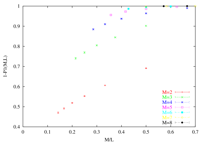
FIG. 2.: $1-P_{1}(M,L)$ versus $\frac{M}{L}$ for $M=2,...,\min\left(L,8\right)$, and $L$ $=$ $4$, $6$, $8$, $10$, $12$, $14$.

This conclusion is strengthened if we look for example to the plot of $P_{1}(2,L)-P_{1}(3,L)$ and $P_{1}(3,L)-P_{1}(4,L)$: the data for those two quantities are shown in figure (3). The droplet model suggestion that these quantities go to zero as a power of $L$ when $L$ goes to infinity does not seem very convincing.

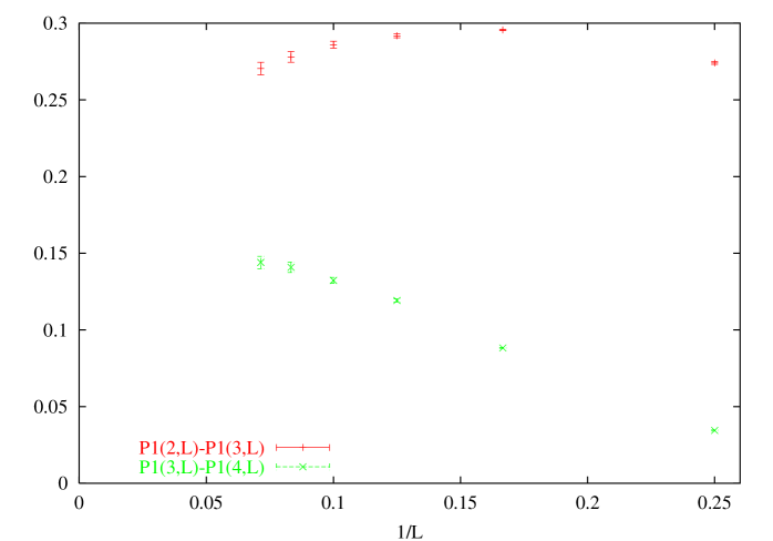
FIG. 3.: The quantities $P_{1}(2,L)-P_{1}(3,L)$ and $P_{1}(3,L)-P_{1}(4,L)$ versus $\frac{1}{L}$ for $L$ $=$ $4$, $6$, $8$, $10$, $12$, $14$.

IV Scaling Behavior

A The Hole Distribution Again

As we have discussed in the introduction if in the infinite volume limit the interface becomes a fractal, characterized by an unique fractal dimension $D_{s}$, and the density of the interface goes to zero as $L^{-\alpha}$, with $\alpha=D-D_{s}$, the probability of finding a hole in a box of size $\cal R$ goes to a non trivial function of $\cal R$ if we keep constant the size of the box in units of $L$. In the opposite case the interface would be become a space filling dense object. If we consider boxes of side $M$ the previous argument shows that the probability that the box does intersect the interface $1-P_{1}(M,L)$ should be a function of $\frac{M}{L}$. A glance to figure (2) shows that our numerical data do not exhibit such scaling: the interface is not a fractal characterized by a simple fractal dimension. On the contrary if we plot $L^{-1.3}\ln(P_{1}(M,L))$ versus $\frac{M}{L}$ (see figure (4) we find a reasonable scaling behavior, indicating again that $1-P_{1}(M,L)$ goes exponentially to $1$ when $L$ goes to infinity at fixed $\frac{M}{L}$.

The same conclusion holds very clearly if we consider the case of boxes of size $L\times L\times 1$, i.e. planes, oriented in the $y-z$ directions, i.e. parallel to the interface. The probability that such a plane does not intersect the interface $P_{p}(L)$ would tend to $1$ in the situation (1) described in section (II A), while it would tend to a non zero number in situation (2), The numerical data (in figure (5)) decrease very rapidly as a function of $L$ (they can be reasonably fitted as $aL^{-\delta}$ with $\delta$ of order two, but a better fit has the form $a\exp(-bL^{c})$: the asymptotic limit is zero in both cases). The first scenario we have presented in section (II A) i.e. the one of an exponent $z<1$, would imply that this probability goes to one asymptotically: this is certainly not the case.

This set of data shows that the interface is space filling on a scale proportional to the side $L$ of the system. Of course one could suggest that the numerical data are affected by very strong corrections to scaling: however it is not clear why this should happen (the scaling in figure (4) is very good). In order to see if we are able to detect any trace of these corrections it is convenient to consider other quantities.

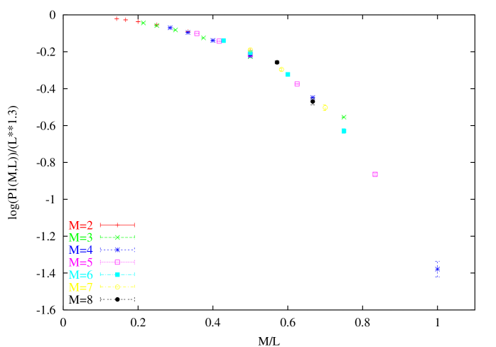
FIG. 4.: $L^{-1.3}\ln(P_{1}(M,L))$ versus $\frac{M}{L}$ for $M=2,...,\min\left(L,8\right)$ and $L$ $=$ $4$, $6$, $8$, $10$, $12$, $14$.

B Other Scaling Laws

If we go back to our boxes of side $M$ we can define the window overlap [10] as the value of the overlap $q$ restricted to one of these boxes. We can define $P_{M,L}(|q|)$ as the probability distribution of the absolute value of such window overlap: the probability is symmetric, so that we can consider only non negative values of $q$. The probability that the interface does not intersect the cube of side $M$ is simply given by $P_{M,L}(1)$.

In the case where the two ground states obtained under different boundary conditions are as different as possible the quantity

$$q^{2}_{M,L}\equiv\int dq\ q^{2}\ P_{M,L}(q)$$ (14)

should go zero at fixed $\frac{M}{L}$ at large $M$. A simple possible scaling behavior is that for large $M$ and $L$

$$q^{2}_{M,L}\simeq L^{-\delta}f(ML^{-1})\ .$$ (15)

We show the numerical data for $q^{2}_{M,L}L^{\delta}$ versus $ML^{-1}$ figure (6) (with $\delta=.32$). The data for $L>4$ show a beautiful and very accurate scaling behavior.

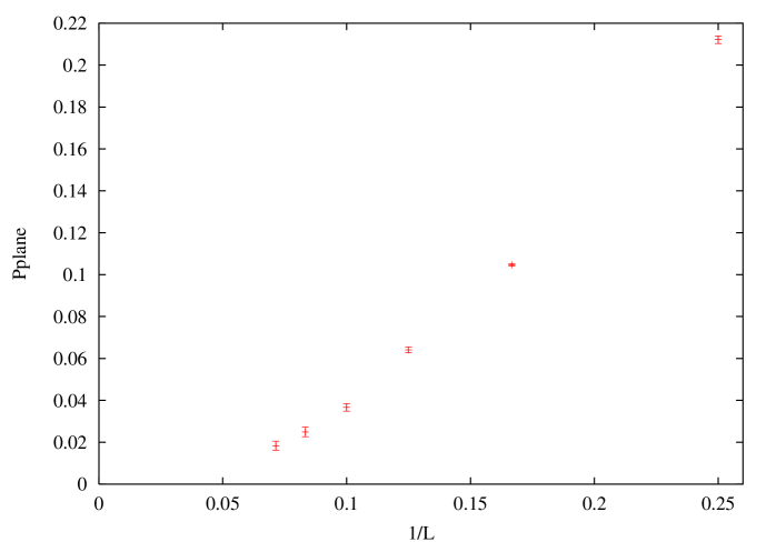
FIG. 5.: $P_{p}(L)$ versus $L^{-1}$ for $L$ $=$ $4$, $6$, $8$, $10$, $12$, $14$.

The data in figures (4) and (6) strongly suggest that asymptotic scaling laws are valid with good accuracy already for the lattice and block sizes that we have considered: sub-leading corrections are small, and they do not seem to be of exceptionally large size. Moreover we find that for windows that occupy a finite fraction of the entire system in the infinite volume limit the window overlap distribution seems to become a delta function $\delta(q)$.

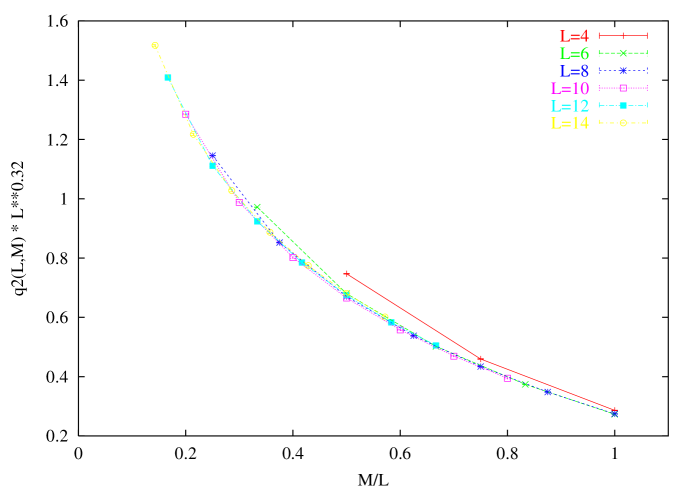
FIG. 6.: $q^{2}_{M,L}L^{\delta}$ versus $ML^{-1}$ for $M=2,...,\min\left(L,8\right)$ and $L$ $=$ $4$, $6$, $8$, $10$, $12$, $14$.

Up to now all of our numerical evidence seems in perfect agreement with the RSB predictions, and the first two possibilities we had discussed in section (II A) are excluded. In order to exclude the more exotic last possibility, and to present further evidence for the correctness of the RSB picture, it is convenient to study the correlation functions, both of $q_{l}$ and of $q$. This will be done in the next section.

V Correlation Functions

A The Link Overlap Correlation Functions

We will present here a detailed analysis of the correlation functions: this is important since they carry a large amount of information that is crucial to distinguish among the different possible behaviors.

As we have already discussed if we consider the case where there is an interface in the $y-z$ plane we must distinguish among correlations in the transverse and in the perpendicular directions. Moreover in the case of vector like quantities like $q_{l}$ we must distinguish among correlations in the direction of the link and correlations in the directions perpendicular to that of the link. For simplicity here we will consider only one correlation, i.e. the transverse link overlap correlation in the direction perpendicular to the link. More precisely the link overlap correlation function we consider is defined as

$$G(d,L)\equiv{1\over 2L^{3}}\sum_{x,y,z}\overline{q_{l}(x,y,z;\hat{y})\ q_{l}(x,y,z+d;\hat{y})+q_{l}(x,y,z;\hat{z})\ q_{l}(x,y+d,z;\hat{z})}\ .$$ (16)

With this definition the correlation functions are periodic functions of $d$ with period $L$, and they are symmetric functions of $d$, so that only the case $0\leq d\leq\frac{L}{2}$ is interesting.

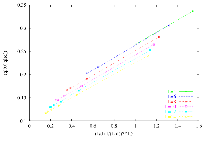
FIG. 7.: The correlation functions $G(d,L)$ versus $w\equiv\left(\frac{1}{d}+\frac{1}{L-d}\right)^{\lambda}$ with $\lambda=1.5$ for $d>0$ and $L$ $=$ $4$, $6$, $8$, $10$, $12$, $14$. The solid curves are smooth interpolations to the data point, and they turn out to be remarkably linear and the lines corresponding to different sizes are nearly parallel.

We show in figure (7) the link overlap correlation functions at distance greater than $0$ for different $L$ values. We plot them as a function of the variable

$$w\equiv\left(\frac{1}{d}+\frac{1}{L-d}\right)^{\lambda}\ ,$$ (17)

with $\lambda=1.5$. The reasons for this choice of the dependent variable will be clearer later: right now we just notice that the points look remarkably linear.

If we want to concentrate our attention on the $d$ dependence of the correlation function (neglecting a possible constant value at large distance) we can consider the quantity

$$\Delta G(d+\frac{1}{2},L)\equiv G(d,L)-G(d+1,L)\ .$$ (18)

Simple scaling implies that the function

$$f(w,L)\equiv\Delta G(d+\frac{1}{2},L)(d^{-1}+(L-d)^{-1})^{1+\lambda}\ ,$$ (19)

where $w=dL^{-1}$, should be independent from $L$ for large $L$. The numerical data are shown in figure (8). A good scaling is obtained with the choice of the value $\lambda=1.5$.

We expect that the correlation function can be fitted at large $L$ and $d$ as

$$G(d,L)=B(L)\left(d^{-1}+(L-d)^{-1}\right)^{-\lambda}+A(L)^{2}\ .$$ (20)

The form that we have taken is the simplest one which enforces the periodicity. Of course different forms are possible. In order to consider also the $d$-independent part of the correlations functions it is convenient to fit the whole set of data shown in figure (7) using equation (20), where for simplicity we fix $\lambda=1.5$. The fits are good (they would also be good for similar values of $\lambda$) so that the whole data can be reconstructed by the knowledge of the parameters $A(L)$ and $B(L)$, which are shown in figure (9).

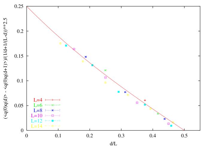
FIG. 8.: The quantity $f(w,L)=\Delta G(d+\frac{1}{2},L)(d^{-1}+(L-d)^{-1})^{1+\lambda}$ with $\lambda=1.5$ as a function of $d$. Here $L$ $=$ $4$, $6$, $8$, $10$, $12$, $14$.

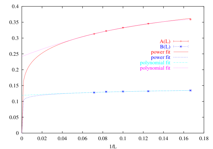
FIG. 9.: The two fit parameters $A(L)$ and $B(L)$ as function of $L$ for $L$ $=$ $4$, $6$, $8$, $10$, $12$, $14$. We show both a a power fit and a polynomial fit in $\frac{1}{L}$.

While $A(L)$ displays some dependence on $L$, there is no hint that the quantity $B(L)$ should go to zero when $L\to\infty$. Certainly both of them do not go to zero as $L^{-\alpha}$ with $\alpha\approx.3$ as expected in the case of possibility (4), and they can be consistently extrapolated to a non-zero value. If we would insist on power law fits we would find a value of $\alpha_{A}=0.15$ for $A(L)$ and a ridiculous value of $\alpha_{B}=0.03$ for $B(L)$.

It is remarkable that $A(L)$, that should tend to the link overlap in the $L\to\infty$ limit, tends to $0.242$, to be compared with the value $0.245\pm 0.015$ (see equation (13)) that we have derived from a completely different analysis: the picture that emerges from these data give consistent support to a RSB physical scenario. Also it is worth to comment more on the power fit of figure (9): even if they are compatible with the data it looks clear they are only minimally consistent with the physical behavior shown by the measured points. Typically these fits stay basically constant for all measured $L$ values, and than they forecast a sharp descend at very high $L$ values: the polynomial fits show on the contrary a consistent behavior in the measured $L$ range and in the $L\to\infty$ limit.

The second scenario we have discussed is in complete variance with the behavior of the correlation function data. The exponent $\lambda$ should be $.3$, not $1.5$, as indicated by the data. This conclusion is in perfect agreement with the results of the hole probability distribution.

We are now ready to analyze the possible correctness of the fourth scenario we have discussed (the interface is a dense set in the continuum limit). The results of figure (8) show that we should have $D_{s}=D-\lambda\approx 1.5$. The fact that the interface would have a fractal dimension less than 2 is strange, but not impossible: the interface could look like the surface of T-lymphocytes, which is full of microvilli, i.e. quasi one dimensional objects.

However in this case the correlation function (and therefore the correlation functions at fixed distance) should go to zero as $L^{-\alpha}$: the correlation functions at distances of order $L$ should go to zero as $L^{-2\alpha}$. The scaling observed in figure (8) should not be there. The two exponents $\alpha_{A}$ and $\alpha_{B}$ should be both equal to $0.3$, which we have already seen it is not true.

It is evident that also the exotic possibility (4) is not compatible with the observed form of the link overlap correlations (which are perfectly compatible with simple scaling laws without anomalies), and the only possibilities is given by the behavior implied by the RSB scenario.

B The Overlap Correlation Functions

Here we consider the overlap correlation function. In this case we can define two interesting correlation functions: the transverse correlation function

$$C_{T}(d,L)={1\over 2L^{3}}\sum_{x,y,z}\overline{q(x,y,z)\ q(x,y,z+d)+q(x,y,z)\ q(x,y+d,z)}\ ,$$ (21)

and the perpendicular correlation function

$$C_{P}(d,L)={1\over L^{3}}\sum_{x,y,z}\overline{q(x,y,z)\ q(x+d,y,z)\ S(x,x+d)}\ ,$$ (22)

where $S(x,x+d)=\pm 1$ is factor which implements gauge invariance: it is equal to $-1$ if the line which connects the points $x$ and $x+d$ crosses the plane where boundary conditions are changed.

The two correlations functions are respectively periodic and anti-periodic functions of $D$ with period $L$ ($C_{P}(L/2,L)=0$).

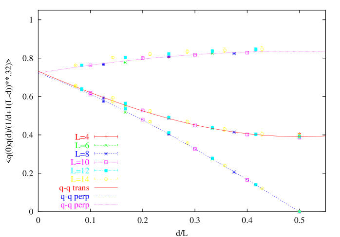
FIG. 10.: The overlap-overlap correlation functions divided times the factor $\left(\frac{1}{d}+\frac{1}{L-d}\right)^{0.32}$ as a function of $\frac{d}{L}$. The upper dots are for the perpendicular correlation function divided an additional factor $(1-\frac{2d}{L})$. Lines are best fits (see the text).

We notice that

$$q_{P}(L)=C_{P}(1,L),\ \ \ \ q_{T}(L)=C_{T}(1,L).$$ (23)

Consequently an analysis of the combined $d$ and $L$ dependence of the overlap-overlap correlation functions can give information on the origin of the $L$ dependence of the link overlap, which coincide with the overlap-overlap correlation function at distance $1$.

According to the previous analysis of the window overlap we expect that the two correlations functions to scale as

$$C(d,L)=f(dL^{-1})(d^{-1}+(L-d)^{-1})^{-\delta}\ .$$ (24)

The plot of figure (10) shows a very good scaling, and two parameter polynomial fits work very well. Transversal and perpendicular correlation functions go to the same limit when $x\to 0$. Since the perpendicular correlation function is identically zero in $d=\frac{L}{2}$, we also plot the perpendicular $C$ divided times $(1-\frac{2d}{L})$, removing in this way the main $\frac{d}{L}$ dependence, which comes from a kinematical effect: it goes very smoothly to the correct limit when $x\to 0$.

The extrapolated values are $0.732\pm 0.008$ for the transverse correlation function and $0.722\pm 0.005$ for the perpendicular one. This is well consistent with the estimate quoted before (and obtained by measuring a completely different quantity) for the link overlap, $q_{l}=0.755\pm 0.015$.

As a consistency check we plot in figure (11) the correlation function $C_{T}(L/2,L)$ as function of $L$. The data can be fitted very well by simple power fit $C\ L^{-\delta}$, with $\delta\simeq 0.32$.

It is clear that we have identified a physical mechanism which naturally generates an $\frac{1}{L}$ dependence in $q_{l}$ (correlation functions do usually feel the size of the system): simple scaling laws are valid and the ground state structure is non trivial. On the contrary a trivial structure (in the sense of the droplet model) would imply that the quantities $f(s)$ extrapolate at $1$ when $s$ goes to zero (which is evidently not true) or they do not satisfy a simple scaling and there is a crossover region of length $\xi(L)$ which goes to infinity with $L$. Both these possibilities are not compatible with the data which strongly suggested the RSB scenario.

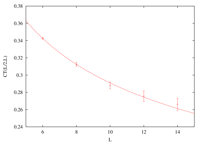
FIG. 11.: The correlation $C_{T}(L/2,L)$ as function $L$ $=$ $4$, $6$, $8$, $10$, $12$, $14$.

VI Conclusions

We have studied the overlap among the two ground states obtained under periodic and anti-periodic boundary conditions for $3D$ lattice of linear sizes $L$ up to $L=14$. We have analyzed many different observables: the average of the link overlap, the probability that the a cube of size $M$ or a plane hits the interface, the window overlap probability distribution and the correlation functions of the link overlap and the overlap.

The droplet model in the usual form assumes that the interface density (which is one minus the link overlap) goes to zero for large $L$ as $L^{-\alpha}$, and that the interface is a fractal with dimension $D^{s}=D-\alpha=3-\alpha$. A small subset of our numerical data is consistent with the possibility the interface density could go to zero as $L^{-\alpha}$, but other data cannot be fitted as a simple power and strongly suggest that the interface density remains finite in the limit $L\to\infty$. The possibility that $D_{s}=3-\alpha$ is completely excluded by the data. Some of the data are compatible with $\alpha=0.3$ and $D_{s}=1.5$, but we have shown that this exotic possibility is not compatible with the rest of data.

The RSB scenario is perfectly compatible with the whole set of data. The appropriate scaling laws for all the variables are satisfied with amazing accuracy. The observed $L$ dependence of the interface density can be easily explained if we consider the scaling law appropriate for the overlap overlap correlation function. We also want to notice the coherence of these results and the recent detection of large scale excitations in spin glass ground states [11, 12].

The behavior we find connects smoothly with the results obtained by simulations at finite temperature [2]. For example we find that the overlap-overlap correlation decays as the distance to a power $\delta=.3$, which is not very far from the value obtained from simulation at finite temperature. Other results in this direction can be found in [13].

We think that we have conclusively shown that the ground state structure of $3D$ Ising spin glasses with Gaussian quenched random couplings is not trivial.

REFERENCES

- [1] G. Parisi, Phys. Rev. Lett. 43, 1754 (1979); J. Phys. A 13, 1101, 1887, L115 (1980); Phys. Rev. Lett. 50, 1946 (1983); M. Mézard, G. Parisi and M. A. Virasoro, Spin Glass Theory and Beyond (World Scientific, Singapore 1987).
- [2] E. Marinari, G. Parisi, F. Ricci Tersenghi, J.J. Ruiz Lorenzo and F. Zuliani, J. Stat. Phys. 98, 973 (2000), cond-mat/9906076.
- [3] H. Rieger, Frustrated Systems: Ground State Properties via Combinatorial Optimization, in Lecture Notes in Physics 501 (Springer-Verlag, Heidelberg 1998).
- [4] J. Houdayer and O. Martin, Phys. Rev. Lett. 83, 1030 (1999), cond-mat/9901276.
- [5] M. Palassini and A. P. Young, Phys. Rev. B 60, R9919 (1999), cond-mat/9904206.
- [6] A. Middleton, Phys. Rev. Lett. 83, 1672 (1999), cond-mat/9904285.
- [7] M. Palassini and A. P. Young, Phys. Rev. Lett. 83, 5126 (1999), cond-mat/9906323.
- [8] E. Marinari and G. Parisi, to be published.
- [9] W. L. McMillan, J. Phys. C 17, 3179 (1984); A. J. Bray and M. A. Moore, in Heidelberg Colloquium on Glassy Dynamics and Optimization, L. Van Hemmen and I. Morgenstern eds. (Springer-Verlag, Heidelberg 1986); D. S. Fisher and D. A. Huse, Phys. Rev. B 38, 386 (1988).
- [10] E. Marinari, G. Parisi, F. Ricci-Tersenghi and J. J. Ruiz-Lorenzo, J. Phys. A 31, L481 (1998).
- [11] F. Krzakala and O. C. Martin, cond-mat/0002055.
- [12] M. Palassini and A. P. Young, cond-mat/0002134.
- [13] E. Marinari, G. Parisi and J. J. Ruiz-Lorenzo, to be published.