Signature of wave localisation in the time dependence of a reflected pulse

Abstract

The average power spectrum of a pulse reflected by a disordered medium embedded in an $N$-mode waveguide decays in time with a power law $t^{-p}$. We show that the exponent $p$ increases from $\frac{3}{2}$ to $2$ after $N^{2}$ scattering times, due to the onset of localisation. We compare two methods to arrive at this result. The first method involves the analytic continuation to imaginary absorption rate of a static scattering problem. The second method involves the solution of a Fokker-Planck equation for the frequency dependent reflection matrix, by means of a mapping onto a problem in non-Hermitian quantum mechanics.

The time-dependent amplitude of a wave pulse reflected by an inhomogeneous medium consists of rapid oscillations with a slowly decaying envelope. The power spectrum $a(\omega,t)$ describes the decay with time $t$ of the envelope of the oscillations with frequency $\omega$. It is a basic dynamical observable in optics, acoustics, and seismology [1]. In the seismological context, the attention has focused on randomly layered media, which are a model for the subsurface of the Earth. The fundamental result of White, Sheng, Zhang, and Papanicolaou [2] for this problem is that $a(\omega,t)$ decays as $t^{-2}$ for times long compared to the scattering time $\tau_{s}$ at frequency $\omega$. The dynamics on this time scale is governed by localisation, since the product of $\tau_{s}$ and the wave velocity $c$ equals the localisation length in one dimension. Although this result for the power spectrum is more than a decade old, it has thus far resisted an extension beyond one-dimensional scattering.

Work towards such an extension by Papanicolaou and coworkers [3, 4] has concentrated on locally layered media, in which the scattering is one-dimensional on short length scales and three-dimensional on long length scales. This is most relevant for seismological applications. Recent dynamical microwave experiments by Genack et al. [5] have motivated us to look at this problem in a wave-guide geometry, in which the scattering is fully three-dimensional — but restricted to a finite number $N$ of propagating waveguide modes. (The single-mode case $N=1$ is statistically equivalent to the one-dimensional model of Ref. [2].) We find that the long-time decay of the average power spectrum is a power law as in the one-dimensional case, but with two exponents: a decay $\propto t^{-3/2}$ crosses over to a $t^{-2}$ decay after a characteristic time $t_{c}=N^{2}\tau_{s}$. The corresponding characteristic length scale $\sqrt{Dt_{c}}$ (with diffusion constant $D$) is the localisation length in an $N$-mode waveguide. The crossover is therefore a dynamical signature of localisation in the reflectance of a random medium, distinct from the signature in the transmittance (or conductance) considered previously in the literature [6, 7, 8].

Let us first formulate the problem more precisely. We consider the reflection of a scalar wave (frequency $\omega$) from a disordered region (length $L$, mean free path $l=c\tau_{s}$) embedded in an $N$-mode waveguide (see Fig. 1, inset). We assume that the length $L$ is greater than the localisation length $\xi=Nl$, so that transmission through the disordered region can be ignored. If in addition the absorption length is greater than $\xi$, the reflection matrix $r(\omega)$ can be regarded as unitary. The matrix product

$$C(\omega,\delta\omega)=r^{\dagger}(\omega-\frac{1}{2}\delta\omega)\ r(\omega+\frac{1}{2}\delta\omega)$$ (1)

is unitary for unitary $r$, so that its eigenvalues are phase factors $\exp(i\phi_{n})$.

The power spectrum for a pulse incident in mode $n$ and detected in mode $m$ is related to $C$ by

$$a(\omega,t) = \int_{-\infty}^{\infty}d\delta t\,e^{i\omega\delta t}\langle r_{mn}(t)r_{mn}(t+\delta t)\rangle$$ (2)

$$= \frac{1}{N}\int_{-\infty}^{\infty}\frac{d\delta\omega}{2\pi}e^{-it\delta\omega}\langle{\rm Tr}\,C(\omega,\delta\omega)\rangle.$$ (3)

(We have normalised $\int dt\,a(\omega,t)=1$.) The phase shifts have the joint distribution function $P(\phi_{1},\phi_{2},\dots,\phi_{N})$. To calculate the average of ${\rm Tr}\,C$ it suffices to know the one-point function $\rho(\phi_{1})\!=\!N\!\int d\phi_{2}\dots\int d\phi_{N}\,P(\mathchoice{{\hbox{\boldmath$\displaystyle\phi$}}}{{\hbox{\boldmath$\textstyle\phi$}}}{{\hbox{\boldmath$\scriptstyle\phi$}}}{{\hbox{\boldmath$\scriptscriptstyle\phi$}}})$, since $\langle{\rm Tr}\,C\rangle=\int d\phi\,\rho(\phi)e^{i\phi}$. We will present two different methods of exact solution. The first method [9] (based on analytic continuation) is simple but restricted to the one-point function, while the second method [2] (based on a Fokker-Planck equation) is more complicated but gives the entire distribution function.

Analytic continuation to the imaginary frequency difference $\delta\omega=i/\tau_{a}$ relates $\exp{(i\phi_{n})}$ to the reflection eigenvalue $R_{n}$ of an absorbing medium with absorption time $\tau_{a}$. The one-point functions are related by

$$\rho(\phi)=\frac{N}{2\pi}+\frac{1}{\pi}\,{\rm Re}\,{\sum\limits_{n=1}^{\infty}e^{-in\phi}}\int\limits_{0}^{1}R^{n}\rho(R)\,dR.$$ (4)

This is a quick and easy way to solve the problem, since $\rho(R)$ is known exactly as a series of Laguerre polynomials [10]. The method of analytic continuation is restricted to the one-point function because averages of negative powers of $\exp{(i\phi_{n})}$ are not analytic in the reflection eigenvalues [9]. For example, for the two-point function one would need to know the average $\langle\exp{(i\phi_{n}-i\phi_{m})}\rangle\to\langle R_{n}R_{m}^{-1}\rangle$ that diverges in the absorbing problem.

The calculation of the power spectrum from Eqs. (3) and (4) is easiest in the absence of time-reversal symmetry, because $\rho(R)$ then has a particularly simple form [10]. We obtain the power spectrum

$$a(\omega,t) = -N^{-1}\theta(t)\,\frac{d}{dt}F\!\left(\frac{t}{2N\alpha\tau_{s}}\right),$$ (6)

$$F(t) = \frac{1}{t+1}\sum\limits_{n=0}^{N-1}\left(\frac{t-1}{t+1}\right)^{n}P_{n}\!\!\left(\frac{t^{2}+1}{t^{2}-1}\right),$$ (7)

where $P_{n}$ is a Legendre polynomial and $\theta(t)$ is the unit step function. The coefficient $\alpha=2,\pi^{2},8/3$ for dimensionality $d=1,2,3$. In the single-mode case Eq. (Signature of wave localisation in the time dependence of a reflected pulse) simplifies to

$$a(\omega,t)=4\tau_{s}(\omega)[t+4\tau_{s}(\omega)]^{-2}\theta(t),$$ (8)

which is the result of White et al. [2]. It decays as $t^{-2}$. For $N\to\infty$ Eq. (Signature of wave localisation in the time dependence of a reflected pulse) simplifies to

$$a(\omega,t)=t^{-1}\exp{[-t/\alpha\tau_{s}(\omega)]}I_{1}[t/\alpha\tau_{s}(\omega)]\theta(t),$$ (9)

where $I_{1}$ is a modified Bessel function. The power spectrum now decays as $t^{-3/2}$. For any finite $N$ we find a crossover from $a=\sqrt{\alpha\tau_{s}/2\pi}\,t^{-3/2}$ for $\tau_{s}\ll t\ll N^{2}\tau_{s}$ to $a=2N\alpha\tau_{s}\,t^{-2}$ for $t\gg N^{2}\tau_{s}$.

In the presence of time-reversal symmetry the exact expression for $a(\omega,t)$ is more cumbersome but the asymptotics carries over with minor modifications. In particular, the large-$N$ limit (9) with its $t^{-3/2}$ decay remains the same, while the $t^{-2}$ decay changes only in the prefactor: $a=(N+1)\alpha\tau_{s}\,t^{-2}$ for $t\gg N^{2}\tau_{s}$.

We now turn to the second method of solution, based on a Fokker-Planck equation for the entire distribution function $P(\mathchoice{{\hbox{\boldmath$\displaystyle\phi$}}}{{\hbox{\boldmath$\textstyle\phi$}}}{{\hbox{\boldmath$\scriptstyle\phi$}}}{{\hbox{\boldmath$\scriptscriptstyle\phi$}}})$. The equation for $N=1$ was derived in Ref. [2]. The multi-mode generalisation can be obtained most directly by analytic continuation of the Fokker-Planck equation for the probability distribution of the reflection eigenvalues — which is known [10]. The resulting Fokker-Planck equation for the phase shifts takes a simple form in the variable $z=\ln\,{\rm cotan}\,{(\phi/4)}\in(-\infty,\infty)$ for $\phi\in(0,2\pi)$. It reads

$$\sum\limits_{n=1}^{N}\frac{\partial}{\partial z_{n}}\left(\frac{\partial P}{\partial z_{n}}-P\frac{\partial\Omega}{\partial z_{n}}\right)=0,$$ (11)

$$\Omega(\mathchoice{{\hbox{\boldmath$\displaystyle z$}}}{{\hbox{\boldmath$\textstyle z$}}}{{\hbox{\boldmath$\scriptstyle z$}}}{{\hbox{\boldmath$\scriptscriptstyle z$}}})=\sum\limits_{n=1}^{N}\left(\ln\cosh{z_{n}}-c_{\beta}\Delta\sinh{z_{n}}\right)$$ (12)

$$\qquad\;\,+\,\,\beta\!\sum\limits_{n>m}\ln\left|\sinh{z_{m}}-\sinh{z_{n}}\right|.$$ (13)

We defined the dimensionless frequency increment $\Delta=\alpha\tau_{s}\delta\omega$ and abbreviated $c_{\beta}=\frac{1}{2}\beta(N-1)+1$. The index $\beta=1(2)$ in the presence (absence) of time-reversal symmetry. We emphasise that, although the Fokker-Planck equation can be obtained by analytic continuation, its solution cannot. Indeed, this would give the solution $P\propto e^{\Omega}$, that fails because it is not normalisable.

We proceed as in Ref.[11] by substituting $P({\mathchoice{{\hbox{\boldmath$\displaystyle z$}}}{{\hbox{\boldmath$\textstyle z$}}}{{\hbox{\boldmath$\scriptstyle z$}}}{{\hbox{\boldmath$\scriptscriptstyle z$}}}})=\Psi({\mathchoice{{\hbox{\boldmath$\displaystyle z$}}}{{\hbox{\boldmath$\textstyle z$}}}{{\hbox{\boldmath$\scriptstyle z$}}}{{\hbox{\boldmath$\scriptscriptstyle z$}}}})\exp{\left[\frac{1}{2}\Omega(\mathchoice{{\hbox{\boldmath$\displaystyle z$}}}{{\hbox{\boldmath$\textstyle z$}}}{{\hbox{\boldmath$\scriptstyle z$}}}{{\hbox{\boldmath$\scriptscriptstyle z$}}})\right]},$ in order to transform the Fokker-Planck equation (Signature of wave localisation in the time dependence of a reflected pulse) into the Schrödinger equation

$$\sum\limits_{n=1}^{N}\Big{[}\!-\!\frac{\partial^{2}}{\partial z^{2}_{n}}+V(z_{n})+\sum\limits_{m\neq n}\!U(z_{n},z_{m})\,\Big{]}\Psi=0,$$ (15)

$$V(z)=c_{\beta}^{2}\left(\frac{\Delta^{2}}{4}\cosh^{2}{z}-\Delta\sinh{z}\right)+\frac{1}{4\cosh^{2}{z}}+V_{0},$$ (16)

$$U(z,z^{\prime})=\frac{1}{2}\beta(\beta-2)\,\frac{\cosh^{2}z+\cosh^{2}z^{\prime}}{\left(\sinh{z}-\sinh{z^{\prime}}\right)^{2}}.$$ (17)

Here $V_{0}=\frac{1}{12}\beta^{2}(N-1)(N-2+6/\beta)+\frac{1}{4}$. By restricting ourselves to $\beta=2$, the interaction term $U$ vanishes and Eq. (Signature of wave localisation in the time dependence of a reflected pulse) has the form of a one-dimensional free-fermion problem. The general solution is given by the Slater determinant

$$\Psi({\mathchoice{{\hbox{\boldmath$\displaystyle z$}}}{{\hbox{\boldmath$\textstyle z$}}}{{\hbox{\boldmath$\scriptstyle z$}}}{{\hbox{\boldmath$\scriptscriptstyle z$}}}})=\,{\rm Det}\,{\left\{\psi_{\mu_{n}}(z_{m})\right\}_{n,m=1}^{N}},$$ (18)

where $\psi_{\mu}(z)$ is an eigenfunction with eigenvalue $\mu$ of the single-particle equation

$$-\psi_{\mu}^{\prime\prime}+V\psi_{\mu}=\mu\psi_{\mu}.$$ (19)

The choice of the eigenfunctions is restricted by the condition $\sum_{n=1}^{N}\mu_{n}=0$ that the total eigenvalue vanishes.

We are now faced with an impasse: The Schrödinger equation (19) has a real spectrum consisting of bound states in the potential well $V(z)$. The bottom of the well is positive for sufficiently large $\Delta$, so that the real spectrum contains only positive $\mu_{n}$’s. How then are we to satisfy the condition of zero sum of the eigenvalues? The way out of this impasse is to allow for complex eigenvalues. The corresponding eigenfunctions will not be square integrable, but that is not a problem as long as the probability distribution $P({\mathchoice{{\hbox{\boldmath$\displaystyle z$}}}{{\hbox{\boldmath$\textstyle z$}}}{{\hbox{\boldmath$\scriptstyle z$}}}{{\hbox{\boldmath$\scriptscriptstyle z$}}}})$ remains normalisable. This is a new twist to the active field of non-Hermitian quantum mechanics [12].

The differential equation (19) is known as the confluent Heun equation [13], but we have found no mention of the complex spectrum in the mathematical physics literature — perhaps because it was considered unphysical. The complex spectrum is constructed by means of a complete set of polynomials to order $N-1$,

$${\cal A}_{\mu}(x)=\sum\limits_{m=1}^{N}g_{m}\,(x-i)^{m-1}(x+i)^{N-m}.$$ (20)

The vector of coefficients ${\mathchoice{{\hbox{\boldmath$\displaystyle g$}}}{{\hbox{\boldmath$\textstyle g$}}}{{\hbox{\boldmath$\scriptstyle g$}}}{{\hbox{\boldmath$\scriptscriptstyle g$}}}}=\{g_{1},g_{2},\dots,g_{N}\}$ is an eigenvector with eigenvalue $\mu$ of the $N\times N$ tri-diagonal matrix $M$, with non-zero elements

$${M}_{nn}=2i\Delta N\!\left(n\!-\!\frac{N+1}{2}\right)\!+\!2\!\left(n\!-\!\frac{N+1}{2}\right)^{2}\!-\frac{N^{2}-1}{6},$$ (21)

$$M_{n,n+1}=n^{2},\qquad M_{n+1,n}=(N-n)^{2}.$$ (22)

Since the trace of $M$ is zero, the condition $\sum_{n}\mu_{n}=0$ is automatically satisfied.

The complex spectrum of Eq. (19) consists of the eigenvalues $\mu_{n}$ with two linearly independent sets of eigenfunctions,

$$\psi^{I}_{\mu}(z) = \sqrt{\cosh{z}}\exp{\left(-\frac{1}{2}N\Delta\sinh{z}\right)}{\cal A}_{\mu}(\sinh{z}),$$ (24)

$$\psi^{II}_{\mu}(z) = \sqrt{\cosh{z}}\exp{\left(\frac{1}{2}N\Delta\sinh{z}\right)}{\cal B}_{\mu}(\sinh{z}).$$ (25)

The functions ${\cal B}_{\mu}$ are related to the polynomials ${\cal A}_{\mu}$ by

$${\cal B}_{\mu}(x)={\cal A}_{\mu}(x)\int\limits_{0}^{\infty}\frac{e^{-N\Delta\,\displaystyle{x^{\prime}}}}{(x-x^{\prime})^{2}+1}{\cal A}_{\mu}^{-2}(x-x^{\prime})\ dx^{\prime}.$$ (26)

The functions ${\cal A}_{\mu}$ and ${\cal B}_{\mu}$ form a bi-orthogonal set on the real axis. We choose the normalisation such that

$$\int_{-\infty}^{\infty}dx\ {\cal A}_{\mu_{n}}(x){\cal B}_{\mu_{m}}(x)=\delta_{nm}.$$ (27)

The solution $\psi^{I}$ of the first kind can not be used because the resulting distribution $P({\mathchoice{{\hbox{\boldmath$\displaystyle z$}}}{{\hbox{\boldmath$\textstyle z$}}}{{\hbox{\boldmath$\scriptstyle z$}}}{{\hbox{\boldmath$\scriptscriptstyle z$}}}})$ is not normalisable. In fact, since

$$\,{\rm Det}\,\left\{{\cal A}_{\mu_{n}}(x_{m})\right\}_{n,m=1}^{N}\propto\prod\limits_{n<m}(x_{n}-x_{m}),$$ (28)

one sees that the substitution of $\psi^{I}$ into Eq. (18) yields the solution $P\propto e^{\Omega}$ that we had rejected earlier. The solution $\psi^{II}$ of the second kind does give a normalisable distribution,

$$P({\mathchoice{{\hbox{\boldmath$\displaystyle z$}}}{{\hbox{\boldmath$\textstyle z$}}}{{\hbox{\boldmath$\scriptstyle z$}}}{{\hbox{\boldmath$\scriptscriptstyle z$}}}})\propto\prod\limits_{n<m}(\sinh{z_{n}}-\sinh{z_{m}})\prod\limits_{i=1}^{N}\cosh{z_{i}}$$ (29)

$$\times\mbox{ }\,{\rm Det}\,{\left\{{\cal B}_{\mu_{n}}(\sinh{z_{m}})\right\}_{n,m=1}^{N}},$$ (30)

or, in terms of the variable $x=\sinh{z}=\,{\rm cotan}\,{(\phi/2)}$,

$$P({\mathchoice{{\hbox{\boldmath$\displaystyle x$}}}{{\hbox{\boldmath$\textstyle x$}}}{{\hbox{\boldmath$\scriptstyle x$}}}{{\hbox{\boldmath$\scriptscriptstyle x$}}}})\propto\,{\rm Det}\,\{{\cal A}_{\mu_{n}}(x_{m})\}_{n,m=1}^{N}\ \,{\rm Det}\,\{{\cal B}_{\mu_{k}}(x_{l})\}_{k,l=1}^{N}.$$ (31)

This is the exact solution of Eq. (Signature of wave localisation in the time dependence of a reflected pulse) for $\beta=2$. Correlation functions of arbitrary order can be obtained from Eq. (31) in terms of a series of the bi-orthogonal functions ${\cal A}_{\mu}$ and ${\cal B}_{\mu}$ [14, 15]. For example, the density of eigenphases $\rho(\phi)$ is given by

$$\rho(\phi)=\frac{dx}{d\phi}\sum\limits_{n=1}^{N}{\cal A}_{\mu_{n}}(x){\cal B}_{\mu_{n}}(x).$$ (32)

Let us examine this solution more closely in various limits. For $N=1$ one has $\mu=0$, ${\cal A}_{\mu}(x)={\rm constant}$, and we reproduce the known single-mode result [2, 16]

$$P(\phi)=\frac{2}{\pi}\tau_{s}\delta\omega(1-\cos\phi)^{-1}{\rm Im}\,e^{\zeta}{\rm Ei}\,(-\zeta),.$$ (33)

Here $\zeta=4i\tau_{s}\delta\omega(1-e^{i\phi})^{-1}$ and Ei is the exponential-integral function. For $N>1$ the eigenvalues $\mu_{n}$ remain real for $\Delta N^{2}\ll 1$. In this regime the integral (26) is easily evaluated, because one can substitute effectively $[(x-x^{\prime})^{2}+1]^{-1}\to\pi\delta(x-x^{\prime})$. Hence ${\cal B}_{\mu}(x)\propto\exp{(-N\Delta\,x)}{\cal A}_{\mu}(x)\,\theta(x)$. Using again Eq. (28), we obtain

$$P({\mathchoice{{\hbox{\boldmath$\displaystyle x$}}}{{\hbox{\boldmath$\textstyle x$}}}{{\hbox{\boldmath$\scriptstyle x$}}}{{\hbox{\boldmath$\scriptscriptstyle x$}}}})\propto\prod\limits_{n<m}(x_{n}-x_{m})^{2}\prod\limits_{i=1}^{N}e^{-N\Delta\,\displaystyle{x_{i}}}\,\theta(x_{i}).$$ (34)

This is the Laguerre ensemble of random-matrix theory. The distribution is dominated by $x\!=\!\,{\rm cotan}\,{(\phi/2)}\gg 1$, so that one can replace $x_{n}\to 2/\phi_{n}$ and recover the result [18] that the inverse time delays, $1/\tau_{n}\equiv\lim_{\delta\omega\to 0}\delta\omega/\phi_{n}$, are distributed according to the Laguerre ensemble. The condition $\Delta N^{2}\ll 1$ for Laguerre statistics means that the characteristic length $L_{\delta\omega}=\sqrt{D/\delta\omega}$ associated with the frequency increment $\delta\omega$ is greater than the localisation length $\xi$. We therefore refer to the regime of validity of Eq. (34) as the localised regime.

At the opposite extreme we have the ballistic regime $L_{\delta\omega}\ll l$, or $\Delta\gg 1$. The integral (26) is now dominated by $x^{\prime}\ll 1$, hence ${\cal B}_{\mu}(x)\propto(x^{2}+1)^{-1}{\cal A}_{\mu}^{-1}(x)$. Moreover, the off-diagonal elements of the matrix $M$ may be neglected so that the polynomials have a simple structure: ${\cal A}_{\mu_{n}}(x)\propto(x+i)^{N-n}(x-i)^{n-1}$. The corresponding functions ${\cal B}$ are given by ${\cal B}_{\mu_{n}}(x)\!=\!\sin^{N+1}{(\phi/2)}\exp{[i\phi(n-N-\frac{1}{2})]}$. The resulting distribution of the eigenphases in the ballistic regime is

$$P({\mathchoice{{\hbox{\boldmath$\displaystyle\phi$}}}{{\hbox{\boldmath$\textstyle\phi$}}}{{\hbox{\boldmath$\scriptstyle\phi$}}}{{\hbox{\boldmath$\scriptscriptstyle\phi$}}}})\propto\prod\limits_{n<m}\left|e^{i\phi_{n}}-e^{i\phi_{m}}\right|^{2},$$ (35)

which we recognize as the circular ensemble of random-matrix theory [17]. This is as expected, since for large $\delta\omega$ the matrix $C$ is the product of two independent reflection matrices $r$, each of which is uniformly distributed in the unitary group. The circular ensemble is the corresponding distribution of the eigenphases.

The intermediate regime $l\ll L_{\delta\omega}\ll\xi$, or $N^{-2}\ll\Delta\ll 1$, is the diffusive one. To study this regime we make a WKB approximation of the Schrödinger equation (19). This approximation requires $N^{2}\Delta\gg 1$ and $N\gg 1$, hence it contains both the ballistic and the diffusive regimes. We obtain

$$\psi^{I,II}_{\mu}(z)=c(\mu)\left(V(z)-\mu\right)^{-1/4}e^{\pm\int_{0}^{z}du\ \sqrt{V(u)-\mu}},$$ (36)

where $c(\mu)$ is a normalisation coefficient. The “$+$” sign in the exponent refers to $\psi_{\mu}^{II}$ and the “$-$” sign to $\psi_{\mu}^{I}$. The eigenvalues $\mu_{n}$ densely fill a curve ${\cal C}$ in the complex plane. We may substitute $\sum_{\mu}f_{\mu}\to\int_{\cal C}\rho(\mu)f(\mu)\,d\mu$, where $\rho(\mu)=N[4\pi ic^{2}(\mu)]^{-1}$ is the eigenvalue density. For analytic $f(\mu)$, the integral along ${\cal C}$ depends only on the end points $\mu_{\pm}=N^{2}(\frac{1}{3}\pm i\Delta)$ of the curve. From Eqs. (Signature of wave localisation in the time dependence of a reflected pulse), (32) and (36) we obtain the eigenphase density

$$\rho(\phi)=\frac{N}{4\pi\sin^{2}{(\phi/2)}}\,{\rm Im}\,\sqrt{\Delta^{2}+2i\Delta(1-e^{-i\phi})}.$$ (37)

This result can be obtained also from Eq. (4) in the limit $N\to\infty$. It is derived here for $\beta=2$, but is actually $\beta$-independent. (The $\beta$-dependent corrections in the diffusive regime are due to weak localisation, and are smaller by a factor $1/N$.) One can check that $\rho(\phi)\to N/{2\pi}$ for $\Delta\gg 1$, as expected in the ballistic regime. In the opposite regime $\Delta\ll 1$ it simplifies to

$$\rho(\phi)=\frac{N\sqrt{\,{\rm cotan}\,{(\phi/4)}}}{4\pi\sin{(\phi/2)}}\sqrt{2\Delta-\frac{\Delta^{2}}{2\sin{(\phi/2)}}},$$ (38)

with the additional restriction: $\sin{(\phi/2)}\geq\Delta/4$. We have plotted Eq. (37) in Fig. 1 for several values of $\Delta$.

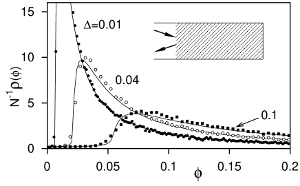
FIG. 1.: Density of the eigenphases for different values of the dimensionless frequency difference $\Delta=\alpha\tau_{s}\delta\omega$. The solid curves are computed from Eq. (37), the data points result from a numerical solution of the wave equation on a two-dimensional square lattice ($\alpha=\pi^{2}/4,N=20$; the scattering time $\tau_{s}$ was obtained independently from the localisation length). The inset shows the geometry of a random medium (shaded) embedded in a waveguide.

In conclusion, we have presented a signature of localisation in the decay of the power spectrum of a pulse reflected by a disordered waveguide. This result is an application of the distribution of the correlator of the reflection matrix at two different frequencies, that we have calculated for arbitrary number of modes $N$, scattering time $\tau_{s}$, and frequency difference $\delta\omega$. With increasing $\delta\omega$ the distribution crosses over from the Laguerre ensemble in the localised regime ($\delta\omega\ll 1/N^{2}\tau_{s}$) to the circular ensemble in the ballistic regime ($\delta\omega\gg 1/\tau_{s}$), via an intermediate “diffusive” regime. The distribution in this intermediate regime does not have the form of any of the ensembles known from random-matrix theory and deserves further study.

This work grew out of an initial investigation of the single-mode case with K. J. H. van Bemmel and P. W. Brouwer. We thank H. Schomerus for valuable discussions. Our research was supported by the Dutch Science Foundation NWO/FOM and by the INTAS grant 97-1342.

REFERENCES

[1]Diffuse Waves in Complex Media, edited by
J.-P. Fouque, NATO Science Series C531 (Kluwer, Dordrecht, 1999).
[2] B. White, P. Sheng, Z. Q. Zhang, and G. Papanicolaou, Phys. Rev. Lett. 59, 1918 (1987).
[3] W. Kohler, G. Papanicolaou, and B. White, in Ref. 1.
[4]
K. Solna and G. Papanicolaou, Waves in Random Media 10, 155 (2000).
[5] A. Z. Genack, P. Sebbah, M. Stoytchev, and B. A. van Tiggelen,
Phys. Rev. Lett. 82, 715 (1999).
[6] B. L. Altshuler, V. E. Kravtsov, and I. V. Lerner,
in Mesoscopic Phenomena in Solids,
edited by B. L. Altshuler, P. A. Lee, and R. A. Webb
(North-Holland, Amsterdam, 1991).
[7] B. A. Muzykantskii and D. E. Khmelnitskii,
Phys. Rev. B 51, 5480 (1995).
[8] A. D. Mirlin, JETP Lett. 62, 603 (1995).
[9] C. W. J. Beenakker, K. J. H. van Bemmel, and P. W. Brouwer,
Phys. Rev. E 60, R6313 (1999).
[10] C. W. J. Beenakker, J. C. J. Paasschens, and P. W. Brouwer,
Phys. Rev. Lett. 76, 1368 (1996);
N. A. Bruce and J. T. Chalker, J. Phys. A 29, 3761 (1996).
[11] C. W. J. Beenakker and B. Rejaei,
Phys. Rev. Lett. 71, 3689 (1993).
[12] N. Hatano and D. R. Nelson,
Phys. Rev. Lett. 77, 570 (1996).
[13]Heun’s Differential Equations, edited by
A. Ronveaux (Clarendon, Oxford, 1995).
[14] K. A. Muttalib, J. Phys. A 28, L159 (1995).
[15] K. Frahm, Phys. Rev. Lett. 74, 4706 (1995).
[16] V. L. Berezinskii and L. P. Gor’kov,
Sov. Phys. JETP 50, 1209 (1979).
[17] M. L. Mehta, Random Matrices
(Academic, New York, 1991).
[18] C. W. J. Beenakker and P. W. Brouwer, preprint
(cond-mat/9908325).