Scaling function for the noisy Burgers equation in the soliton approximation

Abstract

We derive the scaling function for the one dimensional noisy Burgers equation in the two-soliton approximation within the weak noise canonical phase space approach. The result is in agreement with an earlier heuristic expression and exhibits the correct scaling properties. The calculation presents the first step in a many body treatment of the correlations in the Burgers equation.

The strong coupling aspects of driven nonequilibrium systems present an important challenge in statistical physics. The phenomena in question are widespread, including turbulence, interface and growth problems, and chemical reactions.

Here the noisy Burgers equation or equivalently the Kardar-Parisi-Zhang (KPZ) equation, describing the growth of an interface, is one of the simplest models of a driven system showing scaling and pattern formation.

In one dimension the noisy Burgers equation for the slope $u=\nabla h$ of a growing interface has the form [1]

$$\left(\frac{\partial}{\partial t}-\lambda u\nabla\right)u=\nu\nabla^{2}u+\nabla\eta~,$$ (1)

$$\langle\eta(xt)\eta(x^{\prime}t^{\prime})\rangle=\Delta\delta(x-x^{\prime})\delta(t-t^{\prime})~.$$ (2)

The height $h$ is then governed by the KPZ equation [2]

$$\partial h/\partial t=\nu\nabla^{2}h+(\lambda/2)(\nabla h)^{2}+\eta~.$$ (3)

In (1) and (3) $\nu$ is the damping, $\lambda$ the nonlinear mode coupling, and $\eta$ a Gaussian white noise of strength $\Delta$, correlated according to (2). The equation (1) is moreover invariant under the Galilean transformation

$$x\rightarrow x-\lambda u_{0}t~~,~~~u\rightarrow u+u_{0}~.$$ (4)

The Burgers equation (1) and its KPZ equivalent in one and higher dimensions and related models in the same universality class have been studied intensely in recent years owing to their importance as models for a class of nonequilibrium systems [3, 4, 5].

We have in a series of papers analyzed the one dimensional case defined by (1) and (2) in an attempt to uncover the physical mechanisms underlying the pattern formation and scaling behavior [6]. Emphasizing that the noise strength $\Delta$ is the relevant nonperturbative parameter, driving the system into a stationary state, the method was initially based on a weak noise saddle point approximation to the Martin-Siggia-Rose functional formulation [7] of the noisy Burgers equation. This work was a continuation of earlier work based on the mapping of a solid-on-solid model onto a continuum spin model [8]. More recently the functional approach has been superseded by a canonical phase space method [9] deriving from the symplectic structure [10] of the Fokker-Planck equation associated with the Burgers equation.

The functional or the equivalent phase space approach valid in the weak noise limit $\Delta\rightarrow 0$ yields coupled deterministic mean field equations

$$\left(\frac{\partial}{\partial t}-\lambda u\nabla\right)u =\nu\nabla^{2}u-\nabla^{2}p~,$$ (5)

$$\left(\frac{\partial}{\partial t}-\lambda u\nabla\right)p =-\nu\nabla^{2}p~,$$ (6)

for the slope $u$ and a canonically conjugate noise field $p$ (replacing the stochastic noise $\eta$), determining orbits in a canonical phase space and replacing the stochastic Burgers equation (1). The equations (5) and (6) derive from a principle of least action with Hamiltonian density ${\cal H}=p(\nu\nabla^{2}u+\lambda u\nabla u-(1/2)\nabla^{2}p)$ and action $S$ associated with an orbit $u^{\prime}\rightarrow u^{\prime\prime}$ traversed in time $t$,

$$S(u^{\prime\prime},t,u^{\prime})=\int_{0,u^{\prime}}^{t,u^{\prime\prime}}dtdx\left(p\frac{\partial u}{\partial t}-{\cal H}\right)~.$$ (7)

The action is of central importance and serves as a weight for the nonequilibrium configurations (cp. the Boltzmann-Gibbs factor $\exp(-E/kT)$ for equilibrium systems). The action moreover gives access to the time dependent and stationary probability distributions

$$P(u^{\prime\prime},t,u^{\prime})\propto\exp\left[-S(u^{\prime\prime},t,u^{\prime})/\Delta\right]~,$$ (8)

and $P_{\text{st}}(u^{\prime\prime})=\lim_{t\rightarrow\infty}P(u^{\prime\prime},t,u^{\prime})~,$ and associated moments, e.g., the slope correlations

$$\langle uu\rangle(xt)=\int\prod du~u^{\prime\prime}(x)u^{\prime}(0)P(u^{\prime\prime},t,u^{\prime})P_{\text{st}}(u^{\prime})~.$$ (9)

The equations (5) and (6) admit static soliton solutions

$$u_{s}^{\mu}=\mu u\tanh[k_{s}x]~,~~~k_{s}=\lambda u/2\nu~,~~~~\mu=\pm 1~,$$ (10)

moving solitons are generated by the Galilean boost (4). Denoting the right and left boundary values by $u_{+}$ and $u_{-}$, respectively, the velocity is given by

$$u_{+}+u_{-}=-2v/\lambda~.$$ (11)

The index $\mu$ labels the right hand soliton for $\mu=1$ on the ‘noiseless’ manifold $p=0$, also a solution of the damped noiseless Burgers equation for $\eta=0$; and the noise-excited left hand soliton for $\mu=-1$ on the ‘noisy’ manifold $p=2\nu u$, a solution of the growing (unstable) noiseless Burgers equation for $\nu\rightarrow-\nu$. The wavenumber $k_{s}$ sets the inverse length scale. The field equations also admit linear mode solutions superimposed on the solitons; for $\lambda=0$ they become the usual diffusive modes of the driven equation [9].

The physical picture emerging from this analysis is a many body formulation of the pattern formation of a growing interface in terms of a dilute gas of propagating solitons with superimposed linear modes. The formulation also associates energy $E=\int dx{\cal H}$ and momentum $\Pi=\int dxu\nabla p$ with a soliton mode, yielding the dispersion law

$$E\propto(\lambda/\nu^{1/2})\Pi^{z}~,$$ (12)

with dynamic exponent $z=3/2$ and it follows that the strong coupling fixed point features are associated with the soliton dynamics, i.e., defect or domain wall excitations.

In this Letter we pursue the form of the slope correlations (9); the basic building block in the many body formulation. We focus in particular on the scaling function which is of central importance. The dynamic scaling hypothesis [2, 5] and general arguments based on the renormalization group fixed point structure [3, 11] imply the following long time-large distance form of the slope correlations in the stationary state:

$$\langle uu\rangle(xt)=(\Delta/2\nu)x^{-2(1-\zeta)}G\left(x/\xi(t)\right)~.$$ (13)

Here $G$ is the scaling function and $\zeta=1/2$ the roughness exponent inferred from the known stationary probability distribution [12]

$$P_{\text{st}}(u)\propto\exp\left[-(\nu/\Delta)\int dx~u^{2}\right]~.$$ (14)

Within the canonical phase space approach (14) follows from the structure of the zero-energy manifold which attracts the phase space orbits for $t\rightarrow\infty$. The dynamical exponent $z=3/2$ then follows from the scaling law $\zeta+z=2$ implied by the Galilean invariance (4) [2]. In the present approach the exponent $z$ is inferred from the (gapless) soliton dispersion law (12). Finally, the growth of lateral correlations along the interface is characterized by the time dependent correlation length $\xi(t)$. In the nonlinear nonequilibrium Burgers case $\xi(t)$ describes the propagation of solitons and is given by $\xi(t)=\left(\Delta/\nu\right)^{1/3}(\lambda t)^{2/3}$. In the linear equilibrium Edwards-Wilkinson case [13] $\xi(t)$ characterizes the growth of diffusive modes and has the form $\xi(t)=(\nu t)^{1/2}$. It moreover follows from the ‘fluctuation-dissipation theorem’ (14) that $u$ is uncorrelated and that the static correlations have the form, $\langle uu\rangle(x)=(\Delta/2\nu)\delta(x)$, independent of $\lambda$. This is consistent with $\zeta=1/2$ and the limiting form of the scaling function $\lim_{w\rightarrow\infty}G(w)=1$ for $x\gg\xi(t)$. In the dynamical regime for $\xi(t)\gg x$ the correlation decay, i.e., $\langle uu\rangle(x,t)\rightarrow\langle u\rangle\langle u\rangle=0$, and the scaling function vanishes like $G(w)\propto w^{2(1-\zeta)}$ for $w\rightarrow 0$.

Generally, the scaling function can be inferred from the asymptotic properties of the slope correlations (9). In order to evaluate those we must i) determine an orbit from $u^{\prime}$ to $u^{\prime\prime}$ in time $t$ by solving the field equations (5) and (6) as an initial-final value problem in $u$ ($p$ is a slaved variable), ii) evaluate the associated action (7) in order to weigh the orbit and determine $P$ (note that $P_{\text{st}}$ is given by (14)), and, finally, iii) integrate over initial and final configurations $u^{\prime}$ and $u^{\prime\prime}$. Even in the one dimensional case discussed here such a calculation appears rather formidable in the general multi-soliton - linear mode case and we must resort to partial results.

In the weak noise limit the action (7) according to (8) provides a selection criterion determining the dominant dynamical configuration contributing to the distribution. For $\Delta\rightarrow 0$ an important contribution to the growth morphology is constituted by two-soliton configurations or pair excitations

$$u_{2}(x,t)=u^{+}_{s}(x-vt-x_{1})+u^{-}_{s}(x-vt-x_{2})~,$$ (15)

obtained by matching two Galilei-boosted static solitons of opposite parity ($\mu=\pm 1$) (10) centered at $x_{1}$ and $x_{2}$ with soliton separation $\ell=|x_{1}-x_{2}|$ and amplitude $2u$. According to the soliton condition (11) the pair excitation propagates with velocity $v=-\lambda u$ and has vanishing slope field $u=0$ at the boundaries, corresponding to a horizontal interface.

Whereas the solitons (10) for $\mu=\pm 1$ lie on the transient and stationary submanifolds (separatrixes) for $p_{s}=0$ (the ‘noiseless’ kink) and $p_{s}=2\nu u_{s}$ (the ‘noisy’ kink), respectively, and constitute the ‘quarks’ in the many body formulation, the pair excitation (15), satisfying the boundary conditions, is the elementary excitation or ‘quasi particle’ (in the Landau sense) in the present scheme and is characterized by the dispersion law (12). The pair excitation is an approximate solution to the field equations (5) and (6) with a finite lifetime [14]. Over a time scale controlled by the damping $\nu$ the pair decays into diffusive modes; this is consistent with the observation that the phase space orbits approach the zero-energy manifold for $t\rightarrow\infty$.

Unlike a general multi-soliton configuration which changes in time owing to soliton-soliton collisions, the pair excitation preserves its shape over a finite time period, see ref. [9, 14]. Imposing periodic boundary conditions for the slope field the motion of a pair with amplitude $2u$ corresponds to a simple growth mode where the height field $h$, i.e., the integrated slope field, increases layer by layer for each revolution of the soliton pair in a system of size $L$. From the KPZ equation (3) it follows that $\langle dh/dt\rangle=(\lambda/2)\langle u^{2}\rangle$ in a stationary state. Setting $u\rightarrow 2u$ this is consistent with the increase $\Delta h=2u\ell$ during the passage time $\Delta t=\ell/v=\ell/\lambda u$ for a soliton pair of size $\ell$. In Fig. 1 we have depicted the two-soliton growth mode in the slope field $u$ and the associated height field $h$. The pair excitation, which can also be conceived as a bound state composed of two solitons, has the amplitude $2u$, size $\ell$, carries energy $E_{2}=-(16/3)\nu\lambda|u|^{3}$, momentum $\Pi_{2}=-4\nu u|u|$, and action

$$S_{2}=\frac{4}{3}\nu\lambda|u|^{3}t~.$$ (16)

Using the definition (9) it is an easy task to evaluate the contribution to the slope correlations from a single pair. The normalized stationary distribution $P_{\text{st}}$ is obtained from (14) by insertion of (15). Considering the inviscid limit for $\nu\rightarrow 0$ we have

$$P_{\text{st}}(u,\ell)=\Omega^{-1}_{\text{st}}\exp\left[-4(\nu/\Delta)u^{2}\ell\right]~,$$ (17)

$$\Omega_{\text{st}}=(\pi\Delta/\nu)^{1/2}L^{3/2}~.$$ (18)

Correspondingly, inserting (16) in (8) the normalized soliton pair transition probability is

$$P_{\text{sol}}(u,t)=\Omega^{-1}_{\text{sol}}\exp\left[-(4/3)(\nu/\Delta)\lambda|u|^{3}t\right]~,$$ (19)

$$\Omega_{\text{sol}}=(2/3)\Gamma(1/3)[(3/4)(\Delta/\nu)(1/\lambda t)]^{1/3}~.$$ (20)

We note that the normalization factor $\Omega_{\text{st}}$ for the stationary distribution varies as $L^{3/2}$ and that the distribution thus vanishes in the infinite size limit; moreover, the mean size of a pair is equal to $L$, characteristic of an extended excitation (a string). Likewise the transition probability $P_{\text{sol}}$ goes to zero for large times in accordance with the decay of a soliton pair into diffusive modes.

The evolution of $\langle uu\rangle(xt)$ in the two-soliton sector is straightforward. The final configuration $u^{\prime\prime}$ is simply the initial configuration $u^{\prime}$ displaced $vt$ along the axis with no change of shape, i. e., $u^{\prime\prime}(x)=u^{\prime}(x+vt)$, $v=-\lambda u^{\prime}$. Noting that the integral over $u^{\prime}$ and $u^{\prime\prime}=u^{\prime}$ only contributes when the pair configurations overlap and integrating over the size $\ell$ we obtain the slope correlations

$$\langle uu\rangle(xt)=\frac{\ell_{0}}{L}\frac{\int due^{-\frac{4}{3}|u|^{3}\frac{t}{t_{s}}}e^{-4u^{2}|\frac{x}{L}+u\frac{t}{t_{s}}|}C_{1}(u)}{\int due^{-\frac{4}{3}|u|^{3}\frac{t}{t_{s}}}C_{2}(u)}~,$$ (21)

where the cut-off functions originating from the overlap are given by $C_{1}(u)=1/4u^{2}-(1+1/4u^{2})\exp(-4u^{2})$ and $C_{2}(u)=(1/4u^{2})(1-\exp(-4u^{2}))$, respectively. In order to facilitate the discussion of (21) we have introduced the noise-induced length and time scales $\ell_{0}=\Delta/\nu$ and $t_{0}=\Delta/\nu\lambda$; note that $\lambda=\ell_{0}/t_{0}$, and, moreover, the crossover or saturation time $t_{s}=t_{0}(L/\ell_{0})^{3/2}$; the correlation length is then $\xi=\ell_{0}(t/t_{0})^{2/3}$. The expression (21) holds for $t>0$ and is even in $x$ (seen by changing $u$ to $-u$). It samples the soliton pair propagating with velocity $\lambda u$ and is in general agreement with spectral form discussed in the ‘quantum’ treatment in [6]. In Fig. 2 we have shown the two-soliton overlap configurations contributing to the slope correlations.

The weight of single soliton pair is of order $1/L$ and the correlation function $\langle uu\rangle$ thus vanishes in the thermodynamic limit $L\rightarrow\infty$. For a finite system $L$ enters setting a length scale together with the saturation time $t_{s}\propto L^{3/2}$ defining a time scale, and $\langle uu\rangle$ is a function of $x/L$ and $t/t_{s}$ as is the case for the two-soliton expression (21). This dependence should be compared with the wavenumber decomposition of $\langle uu\rangle$ for $\lambda=0$. Here $\langle uu\rangle(xt)\propto(1/L)\sum_{n\neq 0}\exp(-(2\pi n)^{2}t/L^{2})\exp(i\pi nx/L)$, depending on $x/L$ and $t/L^{2}$, corresponding to the saturation time $t_{s}\propto L^{2}$, $z=2$. Keeping only one mode for $n=1$ $\langle uu\rangle$ has the same structure as in the soliton case. In the linear case we can, of course, sum over the totality of modes and in the thermodynamic limit $L\rightarrow\infty$ replace $(1/L)\sum_{n}$ by $\int dk/2\pi$ obtaining the intensive correlations $\langle uu\rangle(xt)=(\Delta/2\nu)(4\pi\nu t)^{-1/2}\exp(-x^{2}/2\nu t)$. Similarly, we expect the inclusion of multi-soliton modes to allow the thermodynamic limit to be carried out yielding an intensive correlation function in the Burgers case.

For a finite system we have in general [15] $\langle uu\rangle(xt)=(1/L)G_{L}(x/L,t/L^{3/2})$ with scaling limits: $G_{L}(x/L,0)\propto\text{const.}$ for $x\sim L$, $G_{L}(x/L,0)\propto L/x$ for $x\ll L$ and $G_{L}(0,t/L^{3/2})\propto\text{const.}$ for $t\gg L^{3/2}$, $G_{L}(0,t/L^{3/2})\propto L/t^{2/3}$ for $t\ll L^{3/2}$. For $L\rightarrow\infty$ we obtain $G_{L}(x/L,t/L^{3/2})\rightarrow(L/x)G(x/t^{2/3})$ in conformity with (13).

It is an important feature of the two-soliton expression (21) that the dynamical soliton interpretation directly implies the correct dependence on the scaling variables $x/L$ and $t/t_{s}\propto t/L^{3/2}$, i.e., independent of a renormalization group argument. However, the scaling limits are at variance with $G_{L}$. Setting, according to (21) $\langle uu\rangle(xt)=(\ell_{0}/L)F(x/L,t/t_{s})$, $F(x/L,0)$ assumes the value $.47$ for $x\ll L$ and decreases monotonically to the value $\sim.08$ for $x\sim L$, whereas $G_{L}$ diverges as $L/x$ for $x\ll L$. Likewise, $F(0,t/t_{s})$ decays from $.47$ for $t\ll t_{s}\propto L^{3/2}$ to $0$ for $t\gg t_{s}$; for $t\sim t_{s}$ we have $F\sim.15$, whereas $G_{L}$ diverges as $L/t^{2/3}$ for $t\ll t_{s}$.

This discrepancy from the scaling limits is a feature the two-soliton contribution which only samples the correlation from a single soliton pair. Moreover, at long times the soliton contribution vanishes and the scaling function is determined by the diffusive mode contribution in accordance with the convergence of the phase space orbits to the stationary zero-energy manifold. We note, however, the general trend towards a divergence for small values of $x$ and $t$ is a feature of $F$.

Introducing the scaling variables $w=x/\xi\propto x/t^{2/3}$ and $\tau=t/t_{s}\propto t/L^{3/2}$ we can also express (21) in the form

$$\langle uu\rangle(xt)=(\ell_{0}/L)F_{2}(w,\tau)~,$$ (22)

where the scaling function $F$ is now given by

$$F(w,\tau)=\frac{\int due^{-\frac{4}{3}|u|^{3}\tau}e^{-4u^{2}|w\tau^{2/3}+u\tau|}C_{1}(u)}{\int due^{-\frac{4}{3}|u|^{3}\tau}C_{2}(u)}~,$$ (23)

and summarize our findings in Fig. 3 where we have depicted $F(w,\tau)$ for a range of $\tau$ values. For fixed small $w=x/\xi\propto x/t^{2/3}$ we have $F\rightarrow.47$ for $\tau=t/t_{s}\propto t/L^{3/2}\rightarrow 0$; for large $\tau$ we obtain $F\rightarrow 0$. The motion of the weak maximum towards smaller values of $w$ for decreasing $\tau$ is a feature of the functional form of $F$ in (23), i.e., the soliton approximation, and probably not a property of the true scaling function which is not expected to have any particularly distinct features [3, 4, 5].

In this Letter we have presented the two-soliton contribution to the slope correlations and ensuing scaling function within the weak noise canonical phase space approach to the noisy Burgers equation in one dimension. The expression is in accordance with a general spectral form proposed earlier on the basis of the many body interpretation of a growing interface and has the correct scaling dependence. This calculation presents the first step in a many body or field theoretical treatment of the correlations in the noisy Burgers equation based on a transparent physical quasi particle picture of the growth mechanisms and ensuing morphology. Details will be presented elsewhere.

Discussions with A. Svane, J. Hertz, B. Derrida, M. Lässig, J. Krug and G. Schütz are gratefully acknowledged.

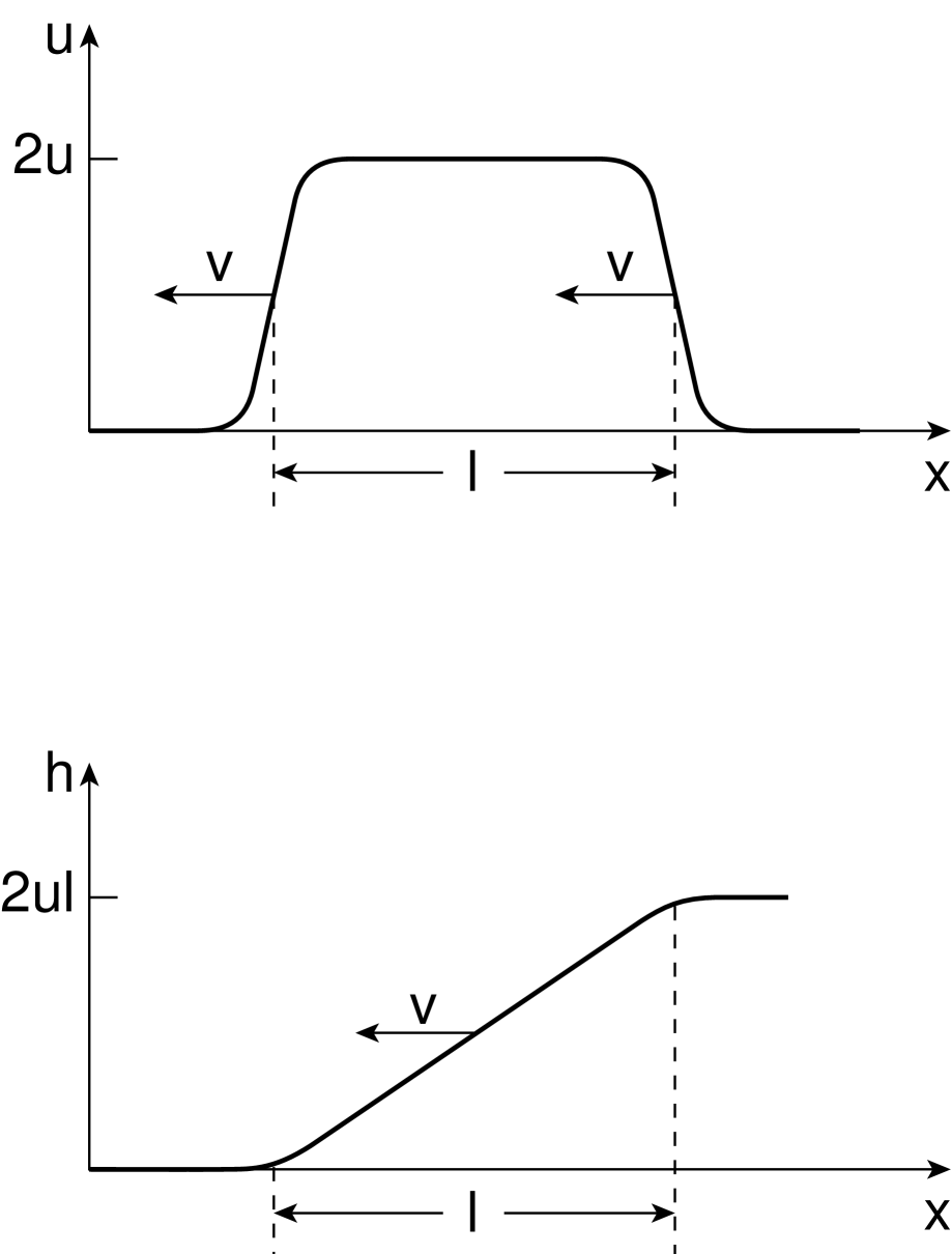
FIG. 1.: The two-soliton growth mode in the slope field $u$ and the associated height field $h$, $u=\nabla h$. The pair soliton excitation has amplitude $2u$ and size $\ell$.

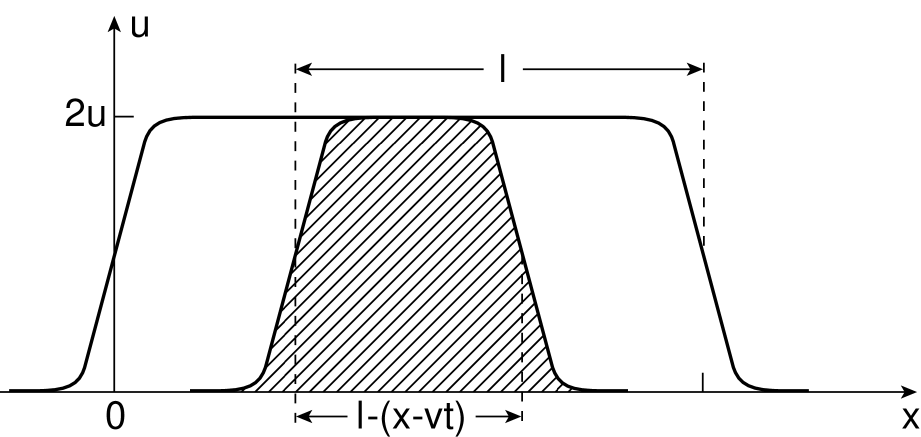
FIG. 2.: The two-soliton configuration of size $\ell$ and amplitude $2u$. The shaded area of size $2\ell-x$ yields a contribution to the slope correlation function.

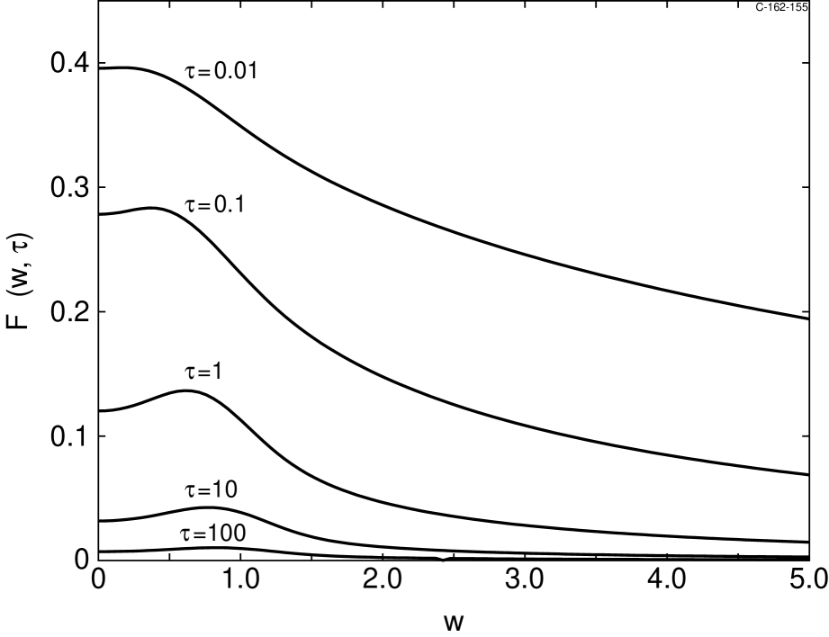
FIG. 3.: Plot of the scaling function $F(w,\tau)$ as a function of the scaling variable $w=x/\xi\propto x/t^{2/3}$ for a range of values of $\tau=t/t_{s}\propto t/L^{3/2}$.

REFERENCES

- [1] D. Forster, D. R. Nelson, and M. J. Stephen, Phys. Rev. Lett. 36, 867 (1976); ibid Phys. Rev. A 16, 732 (1977).
- [2] M. Kardar, G. Parisi, and Y. C. Zhang, Phys. Rev. Lett. 56, 889 (1986); E. Medina, T. Hwa, M. Kardar, and Y. C. Zhang, Phys. Rev. A 39, 3053 (1989).
- [3] T. Hwa and E. Frey, Phys. Rev. A 44, R7873 (1991); E. Frey, U. C. Täuber, and T. Hwa, Phys. Rev. E 53, 4424 (1996).
- [4] U. C. Täuber and E. Frey, Phys. Rev. E 51, 6319 (1995); E. Frey, U. C. Täuber, and H. K. Janssen, Europhys. Lett 47, 14 (1999); M. Lässig, Nucl. Phys. B 448, 559 (1995); M. Lässig, Phys. Rev. Lett. 80, 2366 (1998); M. Lässig, Phys. Rev. Lett. 84, 2618 (2000); M. Prähofer and H. Spohn, Phys. Rev. Lett. 84, 4882 (2000); F. Colaiori and M. A. Moore, Phys. Rev. Lett. 86, 3946 (2001); F. Colaiori and M. A. Moore, Phys. Rev. E 63, 057103 (2001).
- [5] T. Halpin-Healy and Y. C. Zhang, Phys. Rep. 254, 215 (1995).
- [6] H. C. Fogedby, Phys. Rev. E 57, 2331 (1998); H. C. Fogedby, Phys. Rev. E 57, 4943 (1998); H. C. Fogedby, Phys. Rev. Lett. 80, 1126 (1998).
- [7] P. C. Martin, E. D. Siggia, and H. A. Rose, Phys. Rev. A 8, 423 (1973); R. Baussch, H. K. Janssen, and H. Wagner, Z. Phys. B 24, 113 (1976).
- [8] H. C. Fogedby, A. B. Eriksson, and L. V. Mikheev, Phys. Rev. Lett. 75, 1883 (1995).
- [9] H. C. Fogedby, Phys. Rev. E 59, 5065 (1999); H. C. Fogedby, Phys. Rev. E 60, 4950 (1999); H. C. Fogedby, Eur. Phys. J. B 20, 153 (2001).
- [10] M. I. Freidlin and A. D. Wentzel, Random Perturbations of Dynamical Systems (Springer-Verlag, New York, 1984); R. Graham and T. Tél, J. Stat. Phys. 35, 729 (1984); R. Graham, Noise in nonlinear dynamical systems, Vol 1, Theory of continuous Fokker-Planck systems, eds. F. Moss and P. E. V. McClintock (Cambridge University Press, Cambridge, 1989).
- [11] J. Krug, Adv. Phys. 46, 139 (1997).
- [12] D. A. Huse, C. L. Henley, and D. S. Fisher, Phys. Rev. Lett. 55, 2924 (1985).
- [13] S. F. Edwards and D. R. Wilkinson, Proc. Roy. Soc. London A 381, 17 (1982).
- [14] H. C. Fogedby and A. Brandenburg, cond-mat/0105100.
- [15] J. Krug, P. Meakin, and T. Halpin-Healy, Phys. Rev. A 45, 638 (1992); S. Majaniemi, T. Ali-Nissila, and J. Krug, Phys. Rev. B 53, 8071 (1996).