Effective action of a compressible QH state edge: application to tunneling.

Abstract

The electrodynamical response of the edge of a compressible Quantum Hall system affects tunneling into the edge. Using the composite Fermi liquid theory, we derive an effective action for the edge modes interacting with tunneling charge. This action generalizes the chiral Luttinger liquid theory of the Quantum Hall edge to compressible systems in which transport is characterized by a finite Hall angle. In addition to the standard terms, the action contains a dissipative term. The tunneling exponent is calculated as a function of the filling fraction for several models, including screened and unscreened long-range Coulomb interaction, as well as a short-range interaction. We find that tunneling exponents are robust and to a large extent insensitive to the particular model. We discuss recent tunneling measurements in the overgrown cleaved edge systems, and demonstrate that the profile of charge density near the edge is very sensitive to the parameters of the system. In general, the density is nonmonotonic, and can deviate from the bulk value by up to $30\%$. Implications for the correspondence to the chiral Luttinger edge theories are discussed.

Contents

toc

I Introduction

A Background and recent work

The edge of a Quantum Hall (QH) system attracts a lot of interest because it provides an example of a one dimensional non-Fermi-liquid. The theoretical picture of QH edge was first developed for odd-denominator Landau-level filling fractions $\nu$ that correspond to incompressible QH states[1]. It involves one or several interacting chiral Luttinger liquid modes. The most prominent feature of Luttinger liquid is the power law character of the Green’s function.

A power like Green’s function leads to a power law in the tunneling-current–voltage dependence: $I\sim V^{\alpha}$. The tunneling exponent $\alpha$ has been extensively studied theoretically for the principal filling fractions of Laughlin and Jain hierarchies[1, 2]. For Laughlin states with $\nu=1/(2k+1)$ the edge is described by one chiral mode and tunneling current $I\sim V^{2k+1}$ is predicted[1]. Theories of the edge with $\nu\neq 1/(2k+1)$ involve more than one mode. In the multi-mode case the results are qualitatively different for the modes going all in one direction, and for modes going in the opposite directions.

For comoving edge modes, the tunneling exponent is universal and does not depend on the character of interaction between the modes. For example, this is the case at the Jain filling fractions $\nu=n/(np+1)$ with positive integer $n$ and even $p$, where Wen[1] finds $I\sim V^{p+1}$. On the other hand, for the edge described by modes going in opposite directions, the tunneling exponent depends on the interaction strength. In this case, it is also important to take into account the effects of disorder[2]. The point is that relaxation between the modes due to scattering by disorder mixes the modes, and at sufficiently high disorder effectively forms a single charged mode with universal tunneling exponent. For example, for the Jain fractions $n/(np+1)$ with $n<0$ and even $p>0$, Kane, Fisher, and Polchinski[2] found $I\sim V^{p+1-2/|n|}$.

Tunneling experiments probing the physics of the QH edges were first attempted using conventional split gate devices[3], after which a new generation of 2D systems was developed by using the cleaved edge overgrowth technique[4]. In these structures it is possible to study tunneling into the edge of a 2D electron gas from a 3D doped region. In this system one can create a 2DEG with a very sharp edge, with residual roughness of an atomic scale. High quality of the cleaved edge system permits to explore tunneling in both incompressible and compressible QH states[5, 6].

In the first experiment[5], for $\nu=1/3$ it was found that the tunneling conductivity is non-ohmic, $I\sim V^{\alpha}$, with the exponent $\alpha\simeq 2.7$, quite close to the theoretical prediction $\alpha=3$. After that, it was observed[6] that the power law $I\sim V^{\alpha}$ holds for both incompressible and compressible QH densities, in the range $0.25<\nu<1$. The exponent $\alpha$ was found to be reasonably accurately given by a simple formula: $\alpha=1/\nu$. Interestingly, this dependence did not agree with the predictions of chiral Luttinger models, except for a special point $\nu=1/3$. Moreover, it was quite surprising that the power law is equally well obeyed by both compressible and incompressible values of $\nu$.

These findings prompted interest in the problem of tunneling into the edge of a compressible QH system. A good description of the compressible QH states is provided by the composite fermion theory. This theory[7] is constructed at $\nu=1/2$ and other rational $\nu$ with even denominator, and is used to map the problem of fractional QH effect onto the integer QH problem for new quasiparticles, composite fermions interacting via statistical Chern-Simons gauge field. In the composite fermion picture, an electron is described as a fermion carrying vorticity represented by a quantized gauge field vortex. For densities close to the half-filled Landau level the vortex has $p=2$ flux quanta. The theory of composite fermions with $p=2$ describes the interval of densities $1/3<\nu<1$. At smaller densities $1/5<\nu<1/3$ composite fermions with $p=4$ are used, etc.

The theory of tunneling into a compressible QH edge[10] which uses composite fermions to describe the QH system predicts the power law $I\sim V^{\alpha}$, with $\alpha$ being a continuous function of $\nu$:

$$\alpha=1+{e^{2}\over h}\Big{(}\rho_{xy}-|\rho^{(0)}_{xy}|\Big{)},$$ (1)

where $\rho_{xy}=(h/e^{2})\nu^{-1}$ is the Hall resistance of the 2DEG and $\rho^{(0)}_{xy}=(h/e^{2})(\nu^{-1}-p)$ is the Hall resistance of composite fermions moving in an effective magnetic field $B_{\rm eff}=B-p\Phi_{0}n$, where $n$ is electron density. The result (1) describes the system in the limit $\rho_{xx}\to 0$. The dependence of $\alpha$ on $1/\nu$ is monotonic, and is characterized by plateaus in the intervals $2<1/\nu<3$, $4<1/\nu<5$, etc. (see Fig. 2 below). The plateaus are connected by straight lines with slope $2$. The cusp-like singularities predicted in the dependence $\alpha(\nu)$ at $\nu=1/2,\,1/4$, etc., are somewhat smeared when $\rho_{xx}$ is finite (see Eq. (73) and Fig. 2).

Interestingly, these results match exactly the predictions of the chiral Luttinger liquid theory for Jain series of incompressible states. Although formally this theory lacks continuity in the filling fraction, starting from a new set of edge modes for each given filling fraction, the exponents $\alpha(\nu)$ obtained by Wen for $\nu=n/(pn+1)$ and by by Kane, Fisher and Polchinski for $\nu=n/(pn-1)$ fall on the continuous curve (1) found in the composite fermion calculation. The exponents of Wen fall on the plateaus, while those of Kane et al. fall on the straight lines connecting the plateaus.

However, the disagreement with the experimentally measured $\alpha(\nu)$ requires an explanation. Recently a number of theories were proposed trying to resolve this issue. In one approach, described by Conti and Vignale[11], Han and Thouless[12] and Zülicke and MacDonald[13], tunneling is studied by using a hydrodynamical theory of a compressible QH edge, in which the nature of underlying quasiparticles is essentially ignored. From such a treatment the desired relation $\alpha=1/\nu$ emerges readily, as we will discuss in detail below in Sec. I B and at the end of Sec. III. However, this approach ignores the contribution to the electron Green’s function of the quasiparticles in the QH state, and thus it is in contradiction with the presently existing microscopic picture of the QH effect.

Another line of thought, developed by Alekseev et al.[15], is that the experimental system is not what it is assumed to be. In particular, it is proposed that instead of a clean edge the real system contains many localized states in sufficient proximity to the edge. Then, if one assumes that the tunneling rate bottleneck corresponds to tunneling from the doped region into a localized state, and that the density of localized states is sharply peaked about the Fermi energy, one finds the desired result $\alpha=1/\nu$. The reason is that in the problem involving a localized state no conversion of an electron into a quasiparticle is required, and the only effect to be considered is a shakeup of the edge plasmon mode, the effect equivalent to the x-ray edge problem in the Fermi liquid. However, it is not clear why the density of localized states should be peaked at the Fermi energy in the actual samples. An apparently similar idea has been developed earlier by Pruisken et al.[14] using quite elaborate methods which we have not been able to follow in detail.

Also, a theory using composite fermions was proposed by D.-H. Lee and X.-G. Wen[17] in which both charged (edge plasmon) and neutral (quasiparticle) modes are included. It was assumed, however, that the velocity of the charged mode is much larger than the neutral mode velocity. In this case, there exists an intermediate energy regime in which only the charge mode dynamics is important, while the neutral mode response can be ignored. In this energy domain one obtains $\alpha=1/\nu$. It should be pointed out, however, that the ratio of the charged and neutral mode velocities is of order of $\ln w/r_{s}$, where $w$ is the distance from the edge to the doped region, and $r_{s}$ is the screening radius. Optimistically, the ratio $w/r_{s}$ can be as large as $10$ which is still not enough to explain the power law demonstrated in a wide range of $2.5$ decades in the bias voltage.

Another approach trying to rationalize the measured tunneling exponent $\alpha\sim 1/\nu$ was proposed by Khveshchenko[18]. This theory is based on composite fermions and is similar in its assumptions to Ref.[10] and to the present work. However, the calculated tunneling exponent is $1/\nu$ up to a frequency dependent logarithmic correction small in $\rho_{xx}/\rho_{xy}$. We believe that this is due to an inconsistency of the analysis ignoring important effects accounting for dynamics of free composite fermions. One can see that by comparing Eq.7 of Ref.[18] with our Eq.26, and noting that the term describing the free composite fermion response is missing in Ref.[18].

In addition to this controversy, the theory by Lopez and Fradkin[16] seems to abandon the entire theoretical picture of the multi-mode QH edges proposed in Refs.[1, 2] for the incompressible Jain fractions. Unlike Ref.[17], the authors of Ref.[16] are not using a microscopic mechanism for eliminating the neutral propagating edge modes. The construction proposed in Ref.[16] involves only one charged mode plus two auxiliary Klein factors which do not constitute additional propagating degrees of freedom. In that, the approach of Ref.[16] can be comapred to the conventional quantum Hall edge theories[1, 2] in which the velocity of neutral mode is exactly zero. If true, this would lead to the $\alpha=1/\nu$ dependence at arbitrarily low energies. However, it is presently unclear whether the picture of the neutral mode with zero velocity can be justified microscopically.

What complicates the controversy even further is the recently presented evidence of a plateau-like feature exhibited by $\alpha(\nu)$ in some cleaved edge samples[19]. The value of $\nu$ near which the dependence $\alpha(\nu)$ flattens out is however quite close to $1/3$, whereas the expected plateau interval is $2<\nu^{-1}<3$. This discrepancy may be explained by solution of the electrostatic problem near the edge (see Sec. V below and Ref. [19]) which shows that in a wide region adjacent to the edge the density exceeds the bulk value by about $20-30\%$. Because of this behavior of the density profile, the feature in $\alpha(\nu)$ observed near $\nu_{\rm bulk}=1/3$ may correspond to somewhat higher density near the edge, with $\nu$ somewhere between $1/3$ and $1/2$.

One other complication is that the analysis of the electrostatic problem shows that the density profile near the edge can be nonmonotonic and, in general, depends quite sensitively on the system parameters. This observation can make the relation with the theories assuming constant filling factor somewhat indirect. At present, the matter is obviously far from being resolved, and more experimental and theoretical studies are needed to clarify the situation. With this in mind, in this article we present an alternative derivation of the results obtained in Ref.[10], demonstrating their robustness and establishing a more direct connection with the chiral Luttinger theories of the QH edge.

The basis of our analysis will be the theory of composite fermions[7]. We assume that noninteracting composite fermions are characterized by $\rho^{(0)}_{xx}$ and $\rho^{(0)}_{xy}$ which may depend, e.g., on the filling fraction. The measured resistivities are then $\rho_{xy}=\rho^{(0)}_{xy}+ph/e^{2}$ and $\rho_{xx}=\rho^{(0)}_{xx}$, where $p$ is the number of flux quanta attached to an electron ($p=2$ for $1/3<\nu<1$). The tunneling current is expressed in a standard way in terms of the electron Green’s function. We derive the relation between Green’s functions of an electron and of a composite fermion, and compute the former using a “factorization approximation.” In this analysis the effects of shaking up slow electromagnetic and Chern-Simons gauge field modes are separated out. As a result, the tunneling current is expressed in terms of electromagnetic response functions and the number of flux quanta $p$. The theory predicts a power law $I\sim V^{\alpha}$ with a continuous dependence of the tunneling exponent $\alpha$ on the filling fraction. As far as tunneling into the edge is concerned, there is no qualitative difference between compressible and incompressible states. The “Luttinger liquid-like” behavior in the edge tunneling emerges when the Hall angle is close to $\pi/2$, for both compressible and incompressible electron systems.

The paper is organized in the following way. In Sec. I B we review the approach of Ref.[10] based on a semiclassical phase factor analysis of the Green’s function. This is done with the purpose of motivating and providing connection with the subsequent discussion of the effective action formalism. In Sec. II we begin laying out the basic approach of the present theory of tunneling. At low energy, the most important effect is the shake-up of long wavelength modes corresponding to spreading of the tunneling charge. To describe it, one can use a semiclassical method, which provides a simple and universal picture of tunneling[20]. We then construct an effective action in $D=2$ written in terms of composite fermion density and current, as well as the Chern-Simons gauge field. Section II ends by proving an important identity for this action which is used in the following part of the paper.

In this paper we focus on the relatively simple “dirty composite fermion” case, corresponding to composite fermions scattered by the disorder, and described by finite Ohmic conductivity. In Sec. III we consider the problem with short-range interaction between composite fermions. In the $D=2$ action we integrate over the variables in the bulk and derive an effective $D=1$ action that describes the dynamics in terms of the variables at the edge. This action is basically of chiral Luttinger form, with an extra “dissipative” term nonlocal in space and time, which takes into account the effects of charge relaxation in the bulk. The $D=2\ \to\ D=1$ reduction for the problem with short-range CF interaction can be handled in an elementary way and leads to a simple algebraic expression for the tunneling exponent in terms of Ohmic and Hall conductivities.

Then, in Sec. IV we repeat the analysis for the problem with long-range Coulomb interaction. In this case the $D=2\ \to\ D=1$ reduction procedure involves solving a boundary value problem for dynamical screening near the edge. We consider three different models, describing the problems with unscreened Coulomb interaction and also taking into account screening due to image charges induced in the doped overgrown region. (This screening has the peculiarity that the screened interaction remains long ranged, because the image charges are located not above the 2DEG, but on the side of the 2DEG edge.) Two of these boundary value problems can be solved by elementary methods using Fourier transform, and one leads to an integral equation of Wiener-Hopf type. In all three cases, we use the effective $D=1$ action to compute the tunneling current, and derive an expression for the tunneling exponent $\alpha$.

In the case of unscreened interaction the tunneling exponent $\alpha$ turns out to be somewhat frequency dependent, having a contribution proportional to $\rho_{xx}\ln\omega$, which corresponds to a slight deviation from the power law. However, in the most realistic of the three models accounting for screening by the doped region, we find a nearly perfect power law. Otherwise, the results for the three models with long-range interaction, screened and unscreened, and for the short-range interaction model, give essentially the same dependence of the tunneling exponent on $\rho_{xy}$, and thus all agree. The agreement of the results for different kinds of interaction implies that they are robust.

In the calculations described above, we characterize the system by a resistivity tensor that is independent of wave vector and frequency. In particular, this assumption implies that we are restricted to tunneling at voltages and temperatures small compared to the scattering rate of the composite fermions. At energies above the scattering frequency, but below the Fermi energy, one is in a different regime (the “clean regime”) where ballistic dynamics should be used for the composite fermions. This regime may be of considerable practical interest because the samples used for the tunneling measurements are of very high mobility, and are presumably quite clean even near the edge. Even for electron energies below the CF scattering frequency, however, one should really check that contributions from wave vectors larger than the inverse mean free path can safely be ignored.

A proper treatment of the ballistic region requires the use of nonlocal electromagnetic response functions, and is considerably more difficult than the models discussed in the present paper. In the Appendix A below we investigate a simplified model for the nonlocal conductivity, which serves to illustrate some of the salient features of the problem. The simplified model is not adequate, however, to answer unambiguosly the fundamental theoretical question: whether low-energy degrees of freedom at short length scales can significantly alter the tunneling exponent at low electron energies.

In order to better address this problem, we have also undertaken a numerical solution of the charge spreading problem with a proper representation of the nonlocal conductivity. Preliminary results suggest that the tunneling exponents will not be changed by a large amount from the results obtained in the present paper[24], but further work is necessary here.

One should also recall that in the limit of very low temperatures and frequencies, in compressible states, one expects that there will be interaction corrections to the resistivity itself which depend logarithmically on energy [7]. Therefore, in principle, at sufficiently low energies, the renormalized value of $\rho_{xx}$ will become comparable to the value of $\rho_{xy}$ and our entire analysis may cease to be valid. However, the energy range where this would occur is too small to be of experimental interest in high-mobility samples where the bare value of $\rho_{xx}$ is small.

B The semiclassical phase method

The tunneling exponent (1) was derived in Ref.[10] using a “semiclassical phase” approach. Here we restate the derivation of Eq.(1) emphasizing the connection with the effective action method being used in the main part of this article.

One advantage of the semiclassical phase method employed in Ref.[10] is that it does not require subtraction of counterterms like ${\cal S}-{\cal S}_{\rm free}$ used in the following sections. A suspicious reader may think of this subtraction as an ad hoc procedure motivated only on physical grounds. Although we justify the counterterms subtraction carefully and rigorously below in Sec. II C, it will perhaps be useful for the reader to see the same result derived by an alternative method.

It should be mentioned that the phase method, although more appealing intuitively, is more difficult in use, especially in problems with the boundary, like the edge tunneling problem. Because of that our use of it here is limited to the simplest case when the interaction is solely due to the Chern-Simons gauge field, and there is no long-range Coulomb interaction. The short-range interaction is assumed to be taken into account by the composite fermion transformation.

We start with the tunneling electron Green’s function in imaginary time. One can formally write it as an average over the fluctuations of the gauge field:

  

$$G_{{\bf r}\,{\bf r^{\prime}}}(t_{12})={\cal Z}^{-1}\int{\cal D}\{a_{\mu}\}\,G_{{\bf r}\,{\bf r^{\prime}}}(t_{1},t_{2},\,a_{\mu})\,e^{-{\cal L}_{eff}[a_{\mu}]},\qquad t_{12}=t_{2}-t_{1}.$$ (2)

   

This exact expression emphasizes the order of integration over fermionic fields and the gauge field $a_{\mu}$. Here $G_{{\bf r}\,{\bf r^{\prime}}}(t_{1},t_{2},\,a_{\mu})$ is the electron Green’s function for a given configuration of the gauge field $a_{\mu}({\bf r},t)$. For evaluating the tunneling current, we will need $G_{{\bf r}\,{\bf r^{\prime}}}(t_{12})$ for ${\bf r}={\bf r^{\prime}}$.

The effective action ${\cal L}_{eff}[a_{\mu}]$ is the RPA action derived in Ref.[7]. Below we will only need ${\cal L}_{eff}$ up to quadratic order:

$${\cal L}_{eff}[a_{\mu}]=\frac{1}{2}\int a_{\mu}(x){\cal D}^{-1}_{\mu\nu}(x,x^{\prime})a_{\nu}(x^{\prime})\,d^{3}xd^{3}x^{\prime}$$ (3)

where the correlator of gauge field fluctuations ${\cal D}_{\mu\nu}(x,\,x^{\prime})=\langle a_{\mu}(x)\,a_{\nu}(x^{\prime})\rangle$ for the CF system in the absence of long-range interaction in the RPA approximation[7] is given by

$${\cal D}^{-1}_{\mu\nu}(k)={\cal K}_{\mu\nu}(k)+\frac{i}{4\pi p}k^{\lambda}\epsilon_{\mu\nu\lambda}$$ (4)

Here ${\cal K}_{\mu\nu}=\langle j_{\mu}j_{\nu}\rangle$ is the free fermion current correlator (cf. Ref.[7] and Sec.. II below).

We employ a semiclassical approximation for $G_{\bf r\,r}(t_{1},t_{2},\,a_{\mu})$. To motivate it, think of an injected electron which rapidly binds $p$ flux quanta and turns into a composite fermion. The latter moves in the gauge field $a_{\mu}$ and picks up the phase

$$\phi[a_{\mu}]=\int^{\infty}_{-\infty}a^{\mu}({\bf r},\,t)\,j^{\rm free}_{\mu}({\bf r},\,t)\,d^{2}{\bf r}\,dt,$$ (5)

where $j^{\rm free}_{\mu}({\bf r},\,t)$ is the current describing spreading of free composite-fermion density. Semiclassically in $a_{\mu}({\bf r},\,t)$, one writes

$$G_{{\bf r}\,{\bf r}}(t_{1},t_{2},\,a_{\mu})=e^{i\phi[a_{\mu}]}\,G^{(0)}(t_{12}),$$ (6)

where $G^{(0)}(t_{12})\simeq t_{12}^{-1}$ is the composite-fermion Green’s function in the absence of the slow gauge field. Note that fast fluctuations of $a_{\mu}$ are included in $G^{(0)}(t)$ through renormalization of Fermi-liquid parameters.

Let us remind the reader that electron Green’s function in the composite fermion theory has an additional phase factor $\exp\left(i\int^{t_{2}}_{t_{1}}a_{0}(t^{\prime})dt^{\prime}\right)$ introduced by Kim and Wen[23] which accounts for the gauge field of a solenoid inserted into the system upon the transformation of the tunneling electron into a composite fermion. This phase factor has been discussed in the context of the problem of tunneling into the bulk. By virtue of gauge invariance of electron Green’s function under gauge transformations of the Chern-Simons field, one can eliminate the phase factor using the Weil gauge $a_{0}=0$. Because of that, seemingly different approaches to the bulk tunneling problem, some emphasizing the phase factor[23] and others ignoring it[22, 20], are essentially equivalent. Below we are going to use the $a_{0}=0$ gauge, which permits us to drop the solenoid phase factor from the start.

Now, we substitute the Green’s function in the phase approximation (6) into Eq.(2) and average over fluctuations of $a_{\mu}$ using the action (3). This gives

$$G_{{\bf r}\,{\bf r}}(t)=G^{(0)}(t)e^{-S}$$ (7)

where

$$S=\frac{1}{2}\int d^{3}x\,d^{3}x^{\prime}\,j_{\mu}^{\rm free}(x)\,j_{\nu}^{\rm free}(x^{\prime})\,\,{\cal D}_{\mu\nu}(x,x^{\prime}).$$ (8)

It is convenient to rewrite the exponent $S$ hereafter called “action” as follows

$$S=-\frac{i}{2}\int d^{3}xj_{\mu}^{\rm free}(x)\tilde{a}^{\mu}(x)$$ (9)

where $\tilde{a}_{\mu}(x)=i\int{\cal D}_{\mu\nu}(x,x^{\prime})j_{\mu}^{\rm free}(x^{\prime})d^{3}x^{\prime}$ is the actual gauge field produced by the moving charge. The representation (9) follows directly from the ladder structure of the RPA response functions.

From now on we adopt the $a_{0}=0$ gauge, in which the relation between $\tilde{{\bf a}}$ and ${\bf j}$ takes the form

  

$$\tilde{{\bf a}}_{\omega,{\bf k}}=\frac{4\pi pi}{\omega}\,\hat{z}\times{\bf j}_{\omega,{\bf k}},\qquad{\rm i.e.,}\qquad\tilde{{\bf a}}({\bf r},t)=4\pi p\int_{-\infty}^{t}\hat{z}\times{\bf j}({\bf r},t^{\prime})dt^{\prime}.$$ (10)

   

With this, the action $S$ finally becomes

$$S=\sum\limits_{\omega}\frac{2\pi p}{\omega}\left(\int{\bf j}^{\rm free}_{-\omega}({\bf r})\times{\bf j}_{\omega}({\bf r})\,d^{2}r\right)$$ (11)

Note that we are working at $T=0$, and the sum over Matsubara frequencies should actually be interpreted as $\int d\omega/2\pi$. From the form (11) we proceed to evaluate $S$.

The currents ${\bf j}^{\rm free}_{\omega}({\bf r})$ and ${\bf j}_{\omega}({\bf r})$ are found from the diffusion and continuity equations,

$${\bf j}=-\hat{D}\nabla n\ \qquad(\omega-\nabla\hat{D}\nabla)n=J_{\omega}({\bf r})\ ;$$ , (12)

$${\bf j}^{\rm free}=-\hat{D}^{(0)}\nabla n^{\rm free}\ \qquad(\omega-\nabla\hat{D}^{(0)}\nabla)n^{\rm free}=J_{\omega}({\bf r}),$$ , (13)

where $J_{\omega}({\bf r})=e(e^{i\omega t_{1}}-e^{i\omega t_{2}})\delta^{(2)}({\bf r}-{\bf r}_{0})$. The diffusivity and resistivity tensors obey the Einstein relation

$$\hat{D}^{-1}_{\alpha\beta}=\kappa\hat{\rho}_{\alpha\beta},\qquad(\hat{D}^{(0)})^{-1}_{\alpha\beta}=\kappa\hat{\rho}^{(0)}_{\alpha\beta}$$ (14)

where $\kappa$ is compressibility of free composite fermions. (Here “free” indicates the absence of long-range interaction, whereas the short-range interaction is assumed to be present and to give rise to the composite Fermi-liquid physics.)

The resistivity tensors $\rho$ and $\rho^{(0)}$ are related by the composite fermion rule[7]

$$\rho_{\alpha\beta}=\hat{\rho}^{(0)}_{\alpha\beta}+4\pi p\frac{\hbar}{e^{2}}\epsilon_{\alpha\beta}$$ (15)

We remark that, in our notation, the diagonal tensor elements of the imaginary time conductivities, resistivities, and diffusivities have a ${\rm sgn}\,\omega$ dependence on $\omega$ (see Secs. II and III for details). Consequently, we may write ${\hat{D}}(\omega)=-{\hat{D}}^{\rm T}(-\omega)$ and $n_{\omega}({\bf r})=-n_{-\omega}({\bf r})$.

Using these relations, one can simplify the expression for the action as follows:

  

$$S = -\sum\limits_{\omega}\frac{2\pi p}{\omega}\int d^{2}r\left(D^{(0)}_{\alpha^{\prime}\alpha}\nabla_{\alpha^{\prime}}n^{\rm free}_{-\omega}({\bf r})\right)\epsilon_{\alpha\beta}\left(D_{\beta\beta^{\prime}}\nabla_{\beta^{\prime}}n_{\omega}({\bf r})\right)$$ (16)

$$= -\sum\limits_{\omega}\frac{e^{2}}{2h\omega}\int d^{2}r\left(\nabla_{\alpha}n^{\rm free}_{-\omega}({\bf r})\right)\left(\hat{D}^{(0)}(\hat{\rho}-\hat{\rho}^{(0)})\hat{D}\right)_{\alpha\beta}\left(\nabla_{\beta}n_{\omega}({\bf r})\right)$$ (17)

$$= -\sum\limits_{\omega}\frac{e^{2}}{2h\omega}\int d^{2}r\left(\nabla_{\alpha}n^{\rm free}_{-\omega}({\bf r})\right)\left(\kappa\hat{D}^{(0)}-\kappa\hat{D}\right)_{\alpha\beta}\left(\nabla_{\beta}n_{\omega}({\bf r})\right)$$ (18)

$$= -\sum\limits_{\omega}\frac{e^{2}\kappa}{2h\omega}\int d^{2}r\left(n^{\rm free}_{-\omega}({\bf r})\nabla\hat{D}\nabla n_{\omega}({\bf r})-n_{\omega}({\bf r})\nabla\hat{D}^{(0)}\nabla n^{\rm free}_{-\omega}\right)$$ (19)

$$= -\sum\limits_{\omega}\frac{e^{2}\kappa}{2h\omega}\int d^{2}r\left[n^{\rm free}_{-\omega}({\bf r})\left(-\omega+\nabla\hat{D}\nabla\right)n_{\omega}({\bf r})-n_{\omega}({\bf r})\left(-\omega+\nabla\hat{D}^{(0)}\nabla\right)n^{\rm free}_{-\omega}\right]$$ (20)

$$= \sum\limits_{\omega}\frac{e^{2}\kappa}{2h\omega}\int d^{2}r\left(n^{\rm free}_{-\omega}({\bf r})J_{\omega}({\bf r})+J_{-\omega}({\bf r})n_{\omega}({\bf r})\right)$$ (21)

$$= \sum\limits_{\omega}\frac{e^{2}\kappa}{2h\omega}\int d^{2}rJ_{-\omega}({\bf r})\left(n_{\omega}({\bf r})-n^{\rm free}_{\omega}({\bf r})\right)$$ (22)

   

In the above equations, the tensors ${\hat{D}}$ and ${\hat{D}}^{(0)}$ are understood to be always evaluated at frequency $\omega$, not $-\omega$. In going from Eq.(18) to Eq.(19) we were able to discard the boundary term because the currents normal to the boundary are vanishing, as described below. The form (22) will now be used for computing the action.

The density $n_{\omega}({\bf r})$ is found by solving the diffusion equation in the half plane $y>0$, with the boundary condition $j_{y}=-D_{yy}\partial_{y}n-D_{yx}\partial_{x}n=0$ at $y=0$. In Fourier components $n(x,y)=\sum_{k}e^{ikx}n_{k}(y)$ this becomes

$$(\partial^{2}_{y}+q^{2})n_{k}(y)=e(e^{i\omega t_{1}}-e^{i\omega t_{2}})\,\delta(y-y_{0}),$$ (23)

$$D_{yy}\partial_{y}n_{k}(y)_{y\to 0}=-iD_{yx}kn_{k}(0),$$ (24)

where $q=(k^{2}+\omega/D_{xx})^{1/2}$. After solving this elementary boundary value problem we take the limit $y_{0}\to 0$ and have

$$n_{\omega,k}(y)=\frac{e(e^{i\omega t_{1}}-e^{i\omega t_{2}})}{D_{xx}q+iD_{yx}k}\,e^{-qy}$$ (25)

The expression for $n^{\rm free}$ is similar, up to changing $D_{ij}$ to $D^{(0)}_{ij}$.

By inserting $n$ and $n^{\rm free}$ thus found into Eq.(22) one obtains

  

$$S=\frac{e^{2}}{2h}\sum\limits_{\omega,k}\,\frac{|e^{i\omega t_{1}}-e^{i\omega t_{2}}|^{2}}{\omega}\,\left(\frac{1}{\sigma_{xx}q+i\sigma_{yx}k}-\frac{1}{\sigma^{(0)}_{xx}q^{(0)}+i\sigma^{(0)}_{yx}k}\right)$$ (26)

   

Note that this is precisely the expression for the action found in Ref.[10]. Upon evaluating the integrals over $k$ and $\omega$ it gives the result (1) in the limit $\sigma_{xx}\to 0$ and a more general result (1) for finite $\sigma_{xx}$.

Note that the first term in Eq.(26), after integration over $k$ and $\omega$, is a smooth function of $\sigma_{xy}$, whereas the second term gives rise to a cusp in the tunneling exponent at $\sigma^{(0)}_{xy}=0$, i.e, at $\nu=1/2$. Indeed, the first and the second term of Eq.(26) correspond to the first and the second term in Eq.(1), respectively. This means that the plateau in the tunneling exponent for $1/3<\nu<1/2$ arises due to the second term. It is explicit in Eq.(26) that it is the second term that accounts for the free composite fermion dynamics, and so the cusp at $\nu=1/2$ should be understood as a signature of the composite fermion physics.

Let us mention, that the expression (26) for the action can be rewritten as

$$S=\frac{e^{2}}{2h}\sum\limits_{\omega}\frac{\kappa}{\omega}\Big{\langle}J\Bigl{|}\frac{1}{\omega-\nabla\hat{D}\nabla}-\frac{1}{\omega-\nabla\hat{D}^{(0)}\nabla}\Bigr{|}J\Big{\rangle}$$ (27)

This formula can be taken as a hint that the problem of calculating the semiclassical action can be significantly simplified by a wise choice of an effective action and of a compensating counterterm. This is exactly what our strategy will be in the rest of the paper.

II Effective action in $D=2$

A Qualitative discussion

Below we focus on the effect on tunneling arising due to relaxation of collective electrodynamical modes. Semiclassical theory can be used to describe it, assuming that the times and distances controlling the tunneling rate are large.

The adequacy of the semiclassical approach can be understood as follows. Tunneling in a strongly correlated system involves motion of a large number of electrons: While only one electron is actually transferred across the barrier, many other electrons are moving in a correlated fashion to accommodate the new electron. This collective effect becomes progressively more important as the bias decreases. At a small bias $V$, the single-particle barrier traversal time is much shorter than the relaxation time $\tau\sim\hbar/eV$ in the electron liquid. Therefore, while one electron is traversing the barrier other electrons essentially do not move. Thus instantly a large electrostatic potential is formed. The jump in electrostatic energy by an amount much bigger than the bias $eV$ means that right after the one electron transfer we find the system in a classically forbidden state under a collective Coulomb barrier. In order to accomplish tunneling, the charge has to spread over a large area until the potential of the charge fluctuation is reduced below $eV$. If the conductivity is small, the spreading over a large distance takes a long time, and thus the action estimated as the collective barrier height times the relaxation time $\tau$ is much larger than $\hbar$.

This argument fully applies to a composite fermion system consisting of quasiparticles interacting via Coulomb as well as Chern-Simons fields. The tunneling consists of an instant process of adding one electron to the system and of its subsequent slow reaction. The second, cooperative step involving Chern-Simons and Coulomb field relaxation controls the tunneling rate, while the first, single-particle step occurs instantly and contributes only to the prefactor in the tunneling current. Since for small bias the relaxation process occurs on a large scale, one may describe it using the semiclassical approach. However, the fact that the tunneling particle obeys Fermi statistics is also important, and this will be included, finally, in our analysis.

In what follows we treat the system motion under the collective barrier semiclassically as classical Coulomb and Chern-Simons electrodynamics in imaginary time, find an instanton solution, and derive an expression for the tunneling rate in terms of instanton action. For that we generalize to the composite fermion system the semiclassical effective action theory introduced elsewhere[20].

B Constructing the effective action

The effective action can be written in terms of composite fermion charge and current densities $n({\bf r},t)$ and ${\bf j}({\bf r},t)$, as well as the Chern-Simons gauge field $a_{\mu}$. The total action is

$${\cal S}_{total}={\cal S}_{CF}+{\cal S}_{CS}+{\cal S}_{cont}+{\cal S}_{\rm b.c.}$$ (28)

In this section we motivate, define, and discuss different parts of the action (28) for our system.

Below we focus on the case of diffusive CF transport taking place in the presence of disorder. Because the electrical conductivity is local in this case on scales larger than the mean free path, this problem is simpler than that of ballistic CF dynamics.

The assumption underlying our analysis is that the main contribution to the action of the tunneling charge arises from large spatial and time scales, and thus local deviation from equilibrium is small. Therefore, one can expand the action in powers of charge and current densitites, $n({\bf r},t)$ and ${\bf j}({\bf r},t)$, and keep only the terms up to quadratic.

The contribution ${\cal S}_{CF}(n,j)$ is defined to correctly reproduce the equations of motion of composite fermions decoupled from the gauge field $a_{\mu}$ but interacting via the Coulomb potential. [To be more precise, since composite fermions describe interacting electrons in a magnetic field, the short-range part of the Coulomb interaction is included in the definition of $n$ and $j$ of composite fermions, so only the residual long-range part of the Coulomb interaction enters the action ${\cal S}_{CF}(n,j)$.] We consider ${\cal S}_{CF}(n,j)$ of a quadratic form constructed using CF response functions. One can see that the requirement of matching the CF equations of motion is not entirely sufficient to determine the action, e.g., because it leaves freedom of rescaling the whole action or even its different parts corresponding to different normal modes of the problem.

The exact form of the action can be determined in the following way[20]. The action used to study the dynamics in imaginary time is precisely the one that appears in the quantum partition function. The latter action expanded up to quadratic terms in the charge and current density must yield the correct Nyquist spectrum of equilibrium current fluctuations:

$$\langle\!\langle{\bf g}_{\omega,q}^{\alpha}{\bf g}_{-\omega,-q}^{\beta}\rangle\!\rangle=\sigma_{\alpha\beta}|\omega|+\sigma_{\alpha\alpha^{\prime}}D_{\beta\beta^{\prime}}q_{\alpha^{\prime}}q_{\beta^{\prime}}.$$ (29)

Here ${\bf g}(r)={\bf j}(r)+\widehat{D}\nabla n(r)$ is the so-called external current. In this article we are interested in the hydrodynamical regime of small frequency $\omega$ and momentum $q$, in which case the conductivity and diffusivity tensors $\sigma_{\alpha\beta}$ and $D_{\alpha\beta}$ satisfy the Einstein relation $\widehat{\sigma}=e^{2}\kappa_{0}\widehat{D}$, where $\kappa_{0}=dn/d\mu=m^{*}/2\pi\hbar^{2}$ is the free CF compressibility. Generally, both $\widehat{\sigma}$ and $\widehat{D}$ are functions of $\omega$ and $q$.

Below we assume isotropic conductivity tensor characterized by $\sigma_{xx}$ and $\sigma_{xy}$. Also, to make expressions less heavy, we often use the units $\hbar=e=1$ in intermediate steps of calculation, and recover $\hbar$ and $e$ in final results.

The requirement of matching equilibrium current fluctuations is essentially equivalent to the fluctuation-dissipation theorem. The action in imaginary time reads:

  

$${\cal S}_{CF}={1\over 2}\sum\limits_{\omega}\int\!\int\!d^{2}{\bf r}d^{2}{\bf r}^{\prime}\!\left[{\bf g}_{-\omega}^{\alpha}({\bf r})\widehat{K}_{\alpha\beta}(\omega,{\bf r},{\bf r}^{\prime}){\bf g}^{\beta}_{\omega}({\bf r}^{\prime})+U({\bf r}-{\bf r}^{\prime})n_{-\omega}({\bf r})n_{\omega}({\bf r}^{\prime})\right]$$ (30)

where $U({\bf r}-{\bf r}^{\prime})$ is the electron-electron interaction, and the kernel $\widehat{K}(\omega,{\bf r},{\bf r}^{\prime})$ is related to the current-current correlator (29),

$$(K^{-1}_{\omega,q})_{\alpha\beta}=\langle\!\langle{\bf g}_{i\omega,q}^{\alpha}{\bf g}_{-i\omega,-q}^{\beta}\rangle\!\rangle=\sigma^{(0)}_{\alpha\beta}(\omega)\omega+\sigma^{(0)}_{\alpha\alpha^{\prime}}(\omega)D^{(0)}_{\beta\beta^{\prime}}(\omega)q_{\alpha^{\prime}}q_{\beta^{\prime}}$$ (31)

   

given by Eq.(29). Here $\widehat{\sigma}^{(0)}(\omega)$ and $\widehat{D}^{(0)}(\omega)$ are functions of the Matsubara frequency $\omega$ obtained from the real frequency functions by the usual analytic continuation. The superscript $(0)$ here and below indicates that the response functions $\widehat{\sigma}^{(0)}$ and $\widehat{D}^{(0)}$ correspond to the free CF theory, in the absence of coupling to the Chern-Simons field and interaction $U({\bf r}_{1}-{\bf r}_{2})$.

It is appropriate to recall here the general properties of the Matsubara conductivity $\sigma_{\alpha\beta}(\omega)$. By the symmetry of kinetic coefficients, the dielectric function is an even function of the Matsubara frequency: $\epsilon_{\alpha\beta}(i\omega)=\epsilon_{\beta\alpha}(-i\omega)$ (see Ref.[21]). Relating it to conductivity by $\epsilon_{\alpha\beta}(\omega)=\delta_{\alpha\beta}+4\pi\sigma_{\alpha\beta}(\omega)/i\omega$, one obtains that the longitudinal (Ohmic) conductivity is an odd function of $\omega$, while the Hall part is an even function of $\omega$. This means that the constant conductivity case actually corresponds to a discontinuity in $\sigma_{xx}(\omega)$ at $\omega=0$:

$$\sigma_{xx}(i\omega)=\sigma_{xx}\,\mathop{\rm sgn}\nolimits\omega$$ (32)

whereas $\sigma_{xy}(i\omega)=\sigma_{xy}$ has no discontinuity. The same applies to the components of the diffusivity tensor $D_{\alpha\beta}(\omega)$.

The coupling of composite fermion charge and current to the statistical gauge field $a_{\mu}({\bf r},t)$ is described by the Chern-Simons action in a standard way [7]:

$${\cal S}_{CS}=i\int dt\int d^{2}r\Big{(}na_{0}+{\bf j}\cdot{\bf a}+{1\over 4\pi p}\,\varepsilon^{\mu\nu\lambda}a_{\mu}\partial_{\nu}a_{\lambda}\Big{)}$$ (33)

Here $p$ is an even integer corresponding to the number of flux quanta in the construction of composite fermions.

The charge and current densities entering Eqs.(30) and (33) are not independent. They may satisfy a continuity equation. For tunneling problem we employ

$$\dot{n}+\nabla{\bf j}=J({\bf r},t)\,$$ (34)

where the source $J({\bf r},t)=e\delta({\bf r}-{\bf r}_{0})[\delta(t-t_{1})-\delta(t-t_{2})]$ describes adding a composite fermion at the time $t_{1}$ at the point ${\bf r}_{0}$ and subsequently removing it at the time $t_{2}$ at the same point. To handle this constraint, one has to put in the action (28) the term

$${\cal S}_{cont}=i\int\ \left(\dot{n}({\bf r},t)+\nabla{\bf j}({\bf r},t)-J({\bf r},t)\right)\,\Phi({\bf r},t)\ d^{2}r\,dt.$$ (35)

with the Lagrange multiplier function $\Phi({\bf r},t)$.

Finally, to complete the action, one has to ensure proper boundary conditions. We choose the coordinates so that the 2DEG occupies the half plane $y>0$, so that the half plane edge coincides with the $x$-axis. The boundary conditions at the edge arise from the requirement that normal current at the edge vanishes:

$$j_{y}(x,y=0,t)=0$$ (36)

The corresponding part of the action is constructed by using another Lagrange multiplier:

$${\cal S}_{\rm b.c.}=i\int dx\int dt\ j_{y}(x,y=0,t)\phi(x,t)$$ (37)

Besides ensuring proper boundary conditions at $y=0$, the term (37) is needed to make the total action gauge invariant with respect to gauge transformations of the Chern-Simons field $a_{\mu}$.

As remarked in Sec. I B above, we do not need to include in the effective action a term expressing the effect of the solenoid that appears in the system upon the transformation of the electron into a composite fermion. Since we will work in the $a_{0}=0$ gauge, the “string” phase factor $\exp\left(i\int^{t_{2}}_{t_{1}}a_{0}(t^{\prime})dt^{\prime}\right)$ of Kim and Wen[23] is absent.

As a validity check of the action (28) let us derive the dynamical equations. They are obtained by taking the variation of the action (28) with respect to all variables excluding the Lagrange multiplier $\Phi({\bf r},t)$. The resulting equations are of the standard form:

$$\widehat{\rho}^{(0)}{\bf j} = {\bf E}_{CS}-{\bf\nabla}\widetilde{U}n$$ (38)

$${1\over 2\pi p}E^{\alpha}_{CS} = \varepsilon^{\alpha\beta}j^{\beta}$$ (39)

$${1\over 2\pi p}B_{CS} = n+\widetilde{J}$$ (40)

where ${\bf E}_{CS}={\bf\nabla}a_{0}+\dot{{\bf a}}$ and $B_{CS}={\bf\nabla}\times{\bf a}$ are Chern-Simons electric and magnetic fields. The effective interaction $\widetilde{U}$ is defined as

$$\widetilde{U}({\bf r}-{\bf r}^{\prime})=U({\bf r}-{\bf r}^{\prime})+\frac{1}{\kappa_{0}}\delta({\bf r}-{\bf r}^{\prime}),$$ (41)

where $U({\bf r}-{\bf r}^{\prime})$ is the electron-electron interaction and $\kappa_{0}=m_{*}/2\pi\hbar^{2}$ is the compressibility of free composite fermions. Both $\widetilde{U}$ and $\rho^{(0)}$ in Eq.(38) in general act as nonlocal operators. The boundary condition $j_{y}=0$, according to Eq.(39), requires that the tangential Chern-Simons electric field vanishes at the boundary: $\dot{a}_{x}=0$.

Also, it is straightforward to check that eliminating the Chern-Simons field leads to Ohm’s law with a corrected resistivity tensor:

$$\widehat{\rho}{\bf j}=-{\bf\nabla}(\widetilde{U}n),\quad{\rm where}\ \ \widehat{\rho}=\widehat{\rho}^{(0)}+{ph\over e^{2}}\left(\begin{array}[]{cc}0&-1\\ 1&0\end{array}\right)$$ (42)

is the measured resistivity tensor. Note that Chern-Simons interaction changes $\rho_{xy}$, while $\rho_{xx}$ remains intact.

C The fundamental identity

The nonlocal current-current term in Eq.(30) makes a calculation for the problem in the half plane $y>0$ long and not too transparent. To circumvent this algebraic difficulty, we derive an identity for the action (30) that allows us to replace it by an equivalent action with a local current-current term.

To that end, we introduce another CF action:

  

$${\cal S}_{CF}^{\rm loc}={1\over 2}\sum\limits_{\omega}\int d^{2}{\bf r}\,d^{2}{\bf r^{\prime}}\left[{1\over\omega}j^{\alpha}_{-\omega}({\bf r})\rho^{(0)}_{\alpha\beta}({\bf r},{\bf r}^{\prime})j^{\beta}_{\omega}({\bf r}^{\prime})+\widetilde{U}({\bf r}-{\bf r}^{\prime})n_{-\omega}({\bf r})n_{\omega}({\bf r}^{\prime})\right],$$ (43)

   

where $\omega$ is Matsubara frequency. Here $\rho^{(0)}_{\alpha\beta}({\bf r},{\bf r}^{\prime})=\rho^{(0)}_{\alpha\beta}\delta({\bf r}-{\bf r}^{\prime})$ is the resistivity tensor and $\widetilde{U}$ is defined by Eq.(41).

The relation between the actions (30) and (43) is provided by the following fundamental identity:

$${\cal S}_{CF}(n,j)={\cal S}_{CF}^{\rm loc}(n,j)-{\cal S}_{CF}^{\rm loc}(n_{\rm free},j_{\rm free}),$$ (44)

where $n({\bf r},t)$ and $j({\bf r},t)$ are arbitrary functions satisfying the continuity equation (34) and the boundary condition (36), whereas $n_{\rm free}({\bf r},t)$ and $j_{\rm free}({\bf r},t)$ correspond to the saddle point of the action describing noninteracting composite fermions decoupled from the gauge field. Thus the functions $n_{\rm free}$ and $j_{\rm free}$ can be found by solving Eqs. (38)–(40) with $\widetilde{U}({\bf r}-{\bf r}^{\prime})=\kappa_{0}^{-1}\delta({\bf r}-{\bf r}^{\prime})$ and no $E_{CS}$ and $B_{CS}$. Supplemented with the continuity equation that is present in the effective action (28) as a constraint, the equations for $n_{\rm free}$ and $j_{\rm free}$ take the form:

$${\bf j}_{\rm free}({\bf r},\omega)=-\widehat{D}^{(0)}{\bf\nabla}n_{\rm free}({\bf r},\omega);$$ (45)

$$\omega n_{\rm free}({\bf r},\omega)+\nabla j_{\rm free}({\bf r},\omega)=J({\bf r},\omega)$$ (46)

The boundary condition for the system (45) is the absence of normal current $j_{\rm free}$ at $y=0$.

The result (44) is formulated and established below for local resistivity, because in this case the proof is more straightforward. It is possible, however, to generalize it to the case of nonlocal resistivity $\rho^{(0)}_{\alpha\beta}({\bf r},{\bf r}^{\prime})$. This requires more general arguments which will be discussed at the end of this section.

To prove the identity (44), we write the expression (31) for the kernel $\widehat{K}_{\omega}^{-1}$ using gradients:

$$\left(K_{\omega}^{-1}\right)^{\alpha\beta}=\sigma^{\alpha\beta}\omega+\left(\sigma^{\alpha\alpha^{\prime}}\overleftarrow{\nabla}_{\alpha^{\prime}}\right)D^{\beta\beta^{\prime}}\overrightarrow{\nabla}_{\beta^{\prime}}$$ (47)

where the operator convention is that $\overrightarrow{\nabla}_{\alpha}$ acts to the right, whereas $\overleftarrow{\nabla}_{\alpha}$ acts to the left. It is useful to introduce the distinction between $\overrightarrow{\nabla}$ and $\overleftarrow{\nabla}$ and to keep track of it later, so that we are able to invert the kernel $\widehat{K}_{\omega}^{-1}$ and to evaluate the expression in the first term of the action (30) before doing the integral over the half plane. In this way we can properly handle boundary terms.

Inverting Eq.(47) and using the Einstein relation between $D_{\alpha\beta}$ and $\sigma_{\alpha\beta}$ together with the relation between conductivity $\sigma_{\alpha\beta}$ and resistivity $\rho_{\alpha\beta}$, one obtains

$$K_{\alpha\beta}=\frac{\rho_{\alpha\beta}}{\omega}-\overleftarrow{\nabla}_{\alpha}\frac{1}{\kappa_{0}\omega(\omega+\overleftarrow{\nabla}\widehat{D}\overrightarrow{\nabla})}\overrightarrow{\nabla}_{\beta}$$ (48)

Consider the first term in the action (30):

  

$${\bf g}_{-\omega}^{\alpha}K_{\alpha\beta}{\bf g}_{\omega}^{\beta}=\frac{1}{\omega}{\bf g}_{-\omega}^{\alpha}\rho_{\alpha\beta}{\bf g}_{\omega}^{\beta}-\left(\nabla\cdot{\bf g}_{-\omega}\right)\frac{1}{\kappa_{0}\omega(\omega+\overleftarrow{\nabla}\widehat{D}\overrightarrow{\nabla})}\left(\nabla\cdot{\bf g}_{\omega}\right)$$ (49)

Below we perform some manipulations with the expression (49), refraining from integrating over ${\bf r}$ until the very end, because of the above-mentioned need to be careful with gradients and boundary terms.

Now we substitute

$${\bf g}_{\omega}^{\alpha}={\bf j}^{\alpha}+D^{\alpha\beta}(\omega)\nabla_{\beta}n$$ (50)

in the first term of the right-hand side (RHS) of Eq.(49), and find

$$\frac{1}{\omega}{\bf g}_{-\omega}^{\alpha}\rho_{\alpha\beta}{\bf g}_{\omega}^{\beta}=\frac{1}{\omega}j^{\alpha}\rho_{\alpha\beta}j^{\beta}+\frac{1}{\kappa_{0}\omega}\left(j^{\alpha}\nabla_{\alpha}n+(\nabla_{\alpha}n)j^{\alpha}\right)+\frac{1}{\kappa_{0}\omega}n\left(\overleftarrow{\nabla}\widehat{D}\overrightarrow{\nabla}\right)n.$$ (51)

To transform the second term of the RHS of Eq.(49), we substitute

$$\nabla\cdot{\bf g}=\nabla\cdot{\bf j}+\omega n-(\omega+\overleftarrow{\nabla}\widehat{D}\overrightarrow{\nabla})n$$ (52)

and obtain

$$-\left(\nabla\cdot{\bf g}_{-\omega}\right)\frac{1}{\kappa_{0}\omega(\omega+\overleftarrow{\nabla}\widehat{D}\overrightarrow{\nabla})}\left(\nabla\cdot{\bf g}_{\omega}\right)=-J\frac{1}{\kappa_{0}\omega\left(\omega+\overleftarrow{\nabla}\widehat{D}\overrightarrow{\nabla}\right)}J+\frac{1}{\kappa_{0}\omega}(Jn+nJ)-\frac{1}{\kappa_{0}\omega}n\left(\omega+\overleftarrow{\nabla}\widehat{D}\overrightarrow{\nabla}\right)n,$$ (53)

where $J=\nabla\cdot{\bf j}+\omega n$.

Finally, we add the expressions (51) and (53), and combine the last term in Eq.(51) together with the second and third terms of Eq.(53). After doing this we find the resulting expression

$$\frac{1}{\omega}j^{\alpha}\rho_{\alpha\beta}j^{\beta}+\frac{1}{\kappa_{0}}n^{2}-J\frac{1}{\kappa_{0}\omega\left(\omega+\overleftarrow{\nabla}\widehat{D}\overrightarrow{\nabla}\right)}J+\frac{1}{\kappa_{0}\omega}\nabla_{\alpha}\left(j^{\alpha}n+nj^{\alpha}\right)$$ (54)

   

Upon integrating this expression over ${\bf r}$ and multiplying by $1/2$, the first two terms give corresponding terms of the action (43), the third term gives ${\cal S}_{CF}^{\rm loc}(n_{\rm free},j_{\rm free})$ appearing in (44), and the last term vanishes due to the boundary condition (36), thus proving the identity (44)

Having given a formal proof of the identity (44), let us now point out the relation of Eq.(44) to the structure of RPA diagrams in the perturbation theory for Green’s functions in the presence of disorder. To simplify the discussion, let us ignore the CS gauge field, and consider the problem of electrons coupled only by Coulomb interaction. In this case, the RPA self-energy $\Sigma$ can be represented graphically, as shown in Fig. 1. In the $D=2$ problem the bare unscreened interaction, represented in the figure by a thin broken line, is $U({\bf k})=2\pi e^{2}/\epsilon|{\bf k}|$. The diffusive polarization operator is $\Pi({\bf k},\omega)=\kappa_{0}D{\bf k}^{2}/(\omega+D{\bf k}^{2})$, and the diffusive vertex part is $1/(\omega+D{\bf k}^{2})$. One can verify, by performing a resummation, that the dynamically screened interaction, shown in Fig. 1 by a thick black line, can be represented as follows:

  

$$\frac{1}{(\omega+D{\bf k}^{2})^{2}}\,\frac{U({\bf k})}{1+\Pi({\bf k},\omega)U({\bf k})}=\frac{1}{\omega}\left(\frac{1}{D{\bf k}^{2}+\frac{\omega}{1+\kappa_{0}U({\bf k})}}-\frac{1}{D{\bf k}^{2}+\omega}\right),$$ (55)

   

as the difference between the propagator of an auxiliary interaction and the diffusive vertex part, multiplied by $\omega^{-1}$. These two contributions are shown in Fig. 1 by the wavy red and wavy green lines, respectively.

The self-energy diagram in Fig. 1 corresponds to interaction via a dynamically screened Coulomb potential, i.e., to a shakeup of a dissipative plasmon. This effect is described by the hydrodynamical effective action introduced above in Sec. II, and so it is to be expected that the expression in the RHS of Eq.(55) corresponds directly to the difference ${\cal S}^{\rm loc}-{\cal S}^{\rm loc}_{\rm free}$ in Eq.(44).

On can rewrite the formula (55) in a quite general operator form, generalizing it for any interaction $\widehat{U}$, polarization operator $\widehat{\Pi}(\omega)$, and vertex part $\widehat{V}(\omega)$, satisfying the Ward identity $\widehat{\Pi}(\omega)=\kappa_{0}(\widehat{1}-\omega\widehat{V}(\omega))$. For that, one represents the vertex part in the form $\widehat{V}(\omega)=(\widehat{\lambda}+\omega)^{-1}$, and writes:

  

$$\widehat{V}(\omega)\,\left(1+\widehat{U}\widehat{\Pi}(\omega)\right)^{-1}\widehat{U}\,\widehat{V}(\omega)=\frac{1}{\omega}\left(\frac{1}{\widehat{\lambda}+\omega\,(\widehat{1}+\kappa_{0}\widehat{U})^{-1}}-\frac{1}{\widehat{\lambda}+\omega}\right)$$ (56)

   

The formula (56) is proven straightforwardly, by expanding the fractions in operator geometric series, and subsequent resummation.

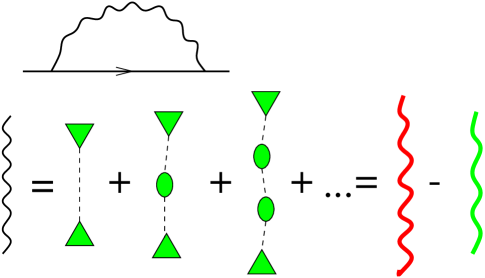
FIG. 1.: Resummation of the RPA diagram series for self-energy for diffusive electrons. The black wavy and broken lines represent dynamically screened interaction and bare unscreened Coulomb interaction, respectively. The bubbles and triangles represent diffusive polarization operators and vertex parts. The red and green wavy lines on the RHS are defined in Eq. 55.

One can view the formulas (55) and (56) as a motivation for the identity (44). More importantly, the relation to RPA diagrams, explicit in Eq.(55) and (56), demonstrates the general character of the identity (44), which is not evident from the way it is justified above. Comparing to Eqs.(55) and (56) makes it clear that the identity (44) is robust under changes in the geometry of the system, alterations of the boundary conditions, and addition of more complicated interactions such as the CS gauge fields.

The analog of Eq.(55) and Eq.(56), and thus of the identity (44), holds even for ballistic Fermi-liquid dynamics. In this case, according to the microscopic theory of Fermi liquid, $\widehat{\Pi}=\kappa_{0}{\bf k}{\bf v}/({\bf k}{\bf v}-\omega)$ and $\widehat{V}=1/(\omega-{\bf k}{\bf v})$, and the operators act on the particle-hole distributions on the Fermi surface. For a Fermi liquid, the formula (56) holds with $\widehat{\lambda}=-{\bf k}{\bf v}$.

III The $D=1$ action for short-range interaction

A Integrating out variables in the bulk

In this section we consider the simplest model of short-range interaction, $U({\bf r}-{\bf r}^{\prime})=U\delta({\bf r}-{\bf r}^{\prime})$, and diffusive CF transport described by $\rho_{\alpha\beta}({\bf r},{\bf r^{\prime}})=\rho_{\alpha\beta}\delta({\bf r}-{\bf r^{\prime}})$.

We shall start with the action ${\cal S}_{total}$ given by Eq.(28) in the half plane and derive an effective $D=1$ problem by integrating out the dynamics in the bulk, and keeping only the variables at the edge. Since the action (28) is quadratic, the integration can easily be performed by the saddle point method.

From now on we replace the CF action (30) by the action (43) with a local current-current term. The virtue of doing this is that the action (43) is much easier to handle, whereas the identity (44) allows us to go back to the physically meaningful action (30) at the very end.

First, it is convenient to integrate out the Chern-Simons gauge field $a_{\mu}$, both in the bulk and at the edge. We do it by fixing the gauge $a_{0}=0$. Upon integration over $a_{\mu}$ the CF resistivity tensor $\rho^{(0)}_{\alpha\beta}$ turns into the electron resistivity tensor (42): $\rho_{xy}=\rho^{(0)}_{xy}+ph/e^{2}$, $\rho_{xx}=\rho^{(0)}_{xx}$. The action acquires the form ${\cal S}_{\rm tot}={\cal S}-{\cal S}_{\rm free}$ with

  

$${\cal S}=\sum\limits_{\omega}\int{d^{2}r\left(\frac{1}{2\omega}\,j_{\alpha,-\omega}\rho_{\alpha\beta}(\omega)j_{\beta,\omega}+\frac{\widetilde{U}}{2}n_{-\omega}({\bf r})n_{\omega}({\bf r})\right)}+{\cal S}_{cont}+{\cal S}_{\rm b.c.}$$ (57)

Then we integrate out $n$ and ${\bf j}$ in the bulk, keeping fixed the normal current $j_{y}$ at the edge. The result is

$${\cal S} = \sum\limits_{\omega}\int{d^{2}r\left(\frac{1}{2}\,\omega\sigma_{\alpha\beta}(\omega)\nabla_{\alpha}\Phi_{-\omega}({\bf r})\nabla_{\beta}\Phi_{\omega}({\bf r})+\frac{\omega^{2}}{2\widetilde{U}}\Phi_{-\omega}({\bf r})\Phi_{\omega}({\bf r})+i\Phi({\bf r},t)\,J({\bf r},t)\right)}$$ (58)

$$+ i\int{dx\,dt\left[\Phi(x,y=0,t)-\phi(x,t)\right]j_{y}(x,y=0,t)}.$$ (59)

Here $\widehat{\sigma}(\omega)=\widehat{\rho}^{-1}(\omega)$ is the electron conductivity tensor. The frequency dependence of $\widehat{\sigma}(\omega)$ is the same as that of $\widehat{\rho}(\omega)$: $\sigma_{xx}(\omega)=\sigma_{xx}{\rm sgn}\omega$, $\sigma_{xy}(\omega)=\sigma_{xy}$, etc.

The next step is to integrate over $j_{y}(y=0)$, which gives $\Phi(x,y=0,t)=\phi(x,t)$. Hence, the action is

$${\cal S}=\sum\limits_{\omega}\int{d^{2}r\left(\frac{1}{2}\,\omega\sigma_{\alpha\beta}(\omega)\nabla_{\alpha}\Phi_{-\omega}({\bf r})\nabla_{\beta}\Phi_{\omega}({\bf r})+\frac{\omega^{2}}{2\widetilde{U}}\Phi_{-\omega}({\bf r})\Phi_{\omega}({\bf r})\right)}+i\int{dx\,dt\,\Phi(x,y=0,t)\,J(x,t)}.$$ (60)

   

In handling the source term $J$ we assume that the point ${\bf r}_{0}=(x_{0},y_{0})$ at which charge is injected is very close to the boundary, i.e., $y_{0}\to 0$, and thus the source in Eq.(60) can be effectively placed at the edge: $J(x,t)=e\delta(x-x_{0})\left[\delta(t-t_{1})-\delta(t-t_{2})\right]$.

Finally, we integrate out the bulk value of $\Phi({\bf r},t)$. From Eq.(60) the equation for $\Phi$ at $y>0$ is

$$\sigma_{xx}(\omega)\nabla^{2}\Phi_{\omega}({\bf r})+\frac{\omega}{\widetilde{U}}\Phi_{\omega}({\bf r})=0.$$ (61)

It is convenient to use the Fourier transform of $\Phi_{\omega}({\bf r})$ with respect to variable $x$ only:

$$\Phi_{\omega}(x,y)=\sum\limits_{k}\Phi_{\omega,k}(y)\,e^{ikx}.$$ (62)

Note that Fourier transform in $y$ is not suitable because we are dealing with the boundary value problem in the $y>0$ domain.

Then the solution to the equation (61) is straightforward:

$$\Phi_{\omega,k}(y)=\Phi_{\omega,k}(y=0)e^{-q(\omega,k)\,y}\ ;$$ (63)

$$q^{2}(\omega,k)=k^{2}+\frac{|\omega|}{\widetilde{U}\sigma_{xx}}.$$ (64)

After substituting Eq.(63) into (60), one obtains a $D=1$ action:

  

$${\cal S}=\sum\limits_{\omega,k}{\frac{1}{2}\left(\sigma_{xx}|\omega|q(\omega,k)+i\sigma_{xy}\,\omega\,k\right)\,\phi_{-\omega,-k}\,\phi_{\omega,k}+J(-\omega,-k)\,\phi_{\omega,k}},$$ (65)

   

where we put Eq.(65) in the Luttinger liquid theory form in terms of the boundary field $\phi(x,t)=\Phi(x,y=0,t)$ introduced above as a Lagrange multiplier.

This effective action represents a generalization of the chiral Luttinger theory of edge modes to the compressible problem with finite $\sigma_{xx}$. Because of the relation between $q$ and $\omega$, the dissipative term in the action (65) is nonlocal in the time representation. In the incompressible limit $\sigma_{xx}\to 0$, we recover the standard chiral Luttinger action:

$${\cal S}={i\nu\over 4\pi}\int\,\partial_{x}\phi\,\partial_{t}\phi\,dx\,dt+i\int J(x,t)\phi dxdt$$ (66)

In the above derivation we ignored effects of the boundary compressibility. Taken into account, these effects lead to an additional term of the form $\int(\partial_{t}\phi)^{2}dxdt$ which does not affect the long-time dynamics and drops from the final answer for the instanton action derived below.

B Instanton action

The source term in the action (65) describes coupling of the tunneling charge to the field $\phi(x,t)$. Thus, the electron creation operator can be written as $\psi^{+}(x,t)=\psi_{CF}^{+}(x,t)e^{ie\phi(x,t)}$, where $\psi_{CF}^{+}(x,t)$ is the operator of a composite fermion, and $e$ is the electron charge. Let us point out the resemblance of the exponential $e^{ie\phi(x,t)}$ to the standard one-dimensional Luttinger liquid expression.

Tunneling is related to the electron Green’s function. To find the tunneling rate, we evaluate the equal point Green’s function $G(\tau)=\langle\psi(0,t_{1})\psi^{+}(0,t_{2})\rangle_{\tau=t_{1}-t_{2}}$ of an electron. Using the above relation of $\psi$ and $\psi_{CF}$, we write the electron Green’s function in terms of the CF operators and then make a factorization approximation:

  

$$\langle\psi(0,t_{1})\psi^{+}(0,t_{2})\rangle=\langle\psi_{CF}(0,t_{1})\psi_{CF}^{+}(0,t_{2})\rangle\Big{\langle}\exp\left(i\int J(x,t)\phi(x,t)dxdt\right)\Big{\rangle},$$ (67)

   

where the first and the second averages on the right-hand side are taken over the fermionic ground state and over fluctuations of the electric and CS gauge fields, respectively. This approximation holds because the dynamics of the injected quasiparticle and of the collective charge relaxation mode are decoupled in space and time. The CF quasiparticles and edge magnetoplasmons differ both in the rate of penetration into the 2DEG bulk and in the velocity of motion along the edge (cf. the discussion in Sec. I B).

Thus the imaginary time Green’s function can be written as

  

$$G(\tau)=G_{CF}(\tau)\,\Big{\langle}\exp\left(i\int J(x,t)\phi(x,t)dxdt\right)\Big{\rangle}=G_{CF}(\tau)\,e^{-[S(\tau)-{\cal S}_{\rm free}(\tau)]},$$ (68)

   

where $G_{CF}(\tau)$ is the Green’s function of a free composite fermion injected and later removed at a point of the boundary. In the last term of Eq.(68) we used the identity (44) relating the average over $\phi(x,t)$ in $\langle\exp\left(i\int J(x,t)\phi(x,t)dxdt\right)\rangle$ to the action (65).

According to the CS Fermi liquid theory, in the effective composite fermion mass approximation, $G_{CF}(\tau)=1/\tau$. This essentially free fermion result holds even though the gauge field fluctuations give rise to infrared-divergent logarithmic corrections[7, 30] to the effective mass $m_{\ast}$, because these corrections are canceled by corrections to the residue $Z$ of the Green’s function.

The tunneling current is obtained from $G(\tau)$ in a standard way. One has to continue $G(\tau)$ from imaginary to real time, and to do the integral over time:

$$I(V)\sim\mathop{\rm Im}\nolimits\int_{0}^{\infty}\,G(t)\,\frac{e^{ieVt}}{t}dt.$$ (69)

Now, we evaluate $\langle\exp\left(i\int J(x,t)\phi(x,t)dxdt\right)\rangle$ using the local action (65). By a Gaussian integration, the result is $e^{-S}$, where

$${\cal S}={1\over 2}\sum\limits_{k,\omega}{|J(\omega)|^{2}\over|\omega|(\sigma_{xx}q+i\sigma_{xy}k\ {\rm sgn}\omega)}$$ (70)

The substitution $k=k_{0}\sinh 2x$ with $k_{0}=(|\omega|/\sigma_{xx}\widetilde{U})^{1/2}$ simplifies integration over $k$:

$${\cal S}={1\over 4}\sum\limits_{\omega}{|J(\omega)|^{2}\over|\omega|}\,\int\frac{(e^{x}+1)dx}{\sigma e^{x}+\sigma^{\ast}},$$ (71)

where $\sigma=\sigma_{xx}+i\sigma_{xy}$. The integral (71) is taken in the domain $-x_{\rm max}<x<x_{\rm max}$, and gives an ultraviolet logarithmically divergent answer which we cut at $k_{\rm max}=k_{0}x_{\rm max}$:

$${\cal S}=\int{d\omega\over|\omega|}|J(\omega)|^{2}\Big{[}{\rho_{xx}\over 8\pi^{2}}\ln{4k^{2}_{\rm max}\sigma_{xx}\widetilde{U}\over|\omega|}+{1\over 4\pi^{2}}\rho_{xy}\theta_{H}\Big{]}$$ (72)

Note that this expression does not vanish even in the absence of interaction with the Chern-Simons field and electron-electron interaction, when $p=0$ and $\widetilde{U}=\kappa_{0}^{-1}$. This indicates that part of the answer represents the contribution of noninteracting composite fermions and must be subtracted off. This subtraction happens automatically because of the identity (44), which confirms that the correct action is indeed $S-{\cal S}_{\rm free}$.

One can see that the counterterm ${\cal S}_{\rm free}$ is indeed related to the effect of free composite fermions. The physical origin of the ultraviolet divergence at $k_{\rm max}$ is that for free fermions the relaxation is fast and involves large momenta $k\sim k_{F}$. On the other hand, the contribution resulting from the interaction should not diverge at large momenta.

To find $S-{\cal S}_{\rm free}$, we subtract from Eq.(72) the same expression with $p=0$ and $\widetilde{U}=\kappa_{0}^{-1}$. Integrating the difference over $\omega$, we get $S-{\cal S}_{\rm free}=(\alpha-1)\ln t/t_{0}$, where $t_{0}$ is a microscopic time of the order of the scattering time, and $\alpha$ is given by

  

$$\alpha=1+{2e^{2}\over\pi h}\Big{[}\theta_{H}\rho_{xy}-\theta^{(0)}_{H}\rho^{(0)}_{xy}\Big{]}+{e^{2}\rho_{xx}\over\pi h}\ln\Big{[}(1+\kappa_{0}U)\sigma_{xx}/\sigma^{(0)}_{xx}\Big{]},$$ (73)

   

where $\theta_{H}=\tan^{-1}\rho_{xy}/\rho_{xx}$ is the Hall angle, $U$ is the short-range interaction, and $\kappa_{0}=m_{\ast}/2\pi\hbar^{2}$ is the free CF compressibility. The behavior of $\alpha$ as a function of $\rho_{xy}$ is displayed in Fig. 2.

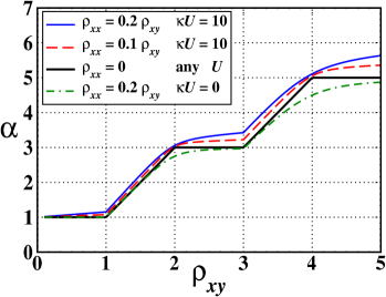
FIG. 2.: The tunneling exponent for the model (41) with short-range interaction $U({\bf r}-{\bf r}^{\prime})=U\delta({\bf r}-{\bf r}^{\prime})$, where $\kappa=\kappa_{0}=m_{\ast}/2\pi\hbar^{2}$.

To verify that $\alpha$ is the tunneling current exponent, we write the electron Green’s function as Eq.(68), where the free composite fermion Green’s function is $G_{CF}(t)\sim t^{-1}$. Therefore, the Green’s function is $G(t)\sim t^{-\alpha}$. One can compute the tunneling current from Eq.(69), and obtain the power law $I(V)\sim V^{\alpha}$. The expression (73) shows that the shake-up effects suppres tunneling in a uniform fashion for the filling factors $\nu$ both on and off the quantum Hall plateaus. The $I-V$ curve is given by a power law with the exponent depending smoothly on the filling factor, via the resistivities $\rho_{xx}$ and $\rho_{xy}$, and effective interaction $\kappa_{0}U$.

One can compare this result with the chiral Luttinger liquid theories of tunneling into the edge of an incompressible QH state. For that, one has to consider the limit of a large Hall angle: $\theta_{H}=\theta^{(0)}_{H}=\pi/2$. In this case $\rho_{xx}\to 0$ and the exponent (73) acquires the form (1) corresponding to a staircase with plateaus in the intervals $1/3<\nu<1/2$, $1/5<\nu<1/4$, etc., interpolated by straight lines with the slope $2$. At the rational filling fractions $\nu=n/(pn\pm 1)$ we recover the results of the Luttinger liquid theories. To see this, substitute $\rho_{xy}=(p+1/n)h/e^{2}$, $\rho^{(0)}_{xy}=h/ne^{2}$ in the expression (1), and get $I\sim V^{1+|p+1/n|-1/|n|}$, which agrees with the universal tunneling exponents predicted by Wen and by Kane, Fisher, and Polchinski for Jain filling factors with positive and negative $n$.

It is interesting that the tunneling exponent (1) has cusplike singularities near the compressible rational $\nu$’s with even denominator, $\nu=1/2,\,1/4$, etc. The origin of this effect is a qualitative change in the structure of the edge modes near these filling factors. In particular, let us discuss the vicinity of $\nu=1/2$, where the quantum Hall state can be described as a Fermi liquid of composite fermions carrying $p=2$ flux quanta each, and exposed to “residual” magnetic field $\delta B=(2-\nu^{-1})$. At $\nu<1/2$ the residual field direction coincides with the total field, and all edge modes propagate in the same direction. On the other hand, at $\nu>1/2$, the structure of the edge is qualitatively different, consisting of modes going in opposite directions. This effect makes $\nu=1/2$ a singular density from the point of view of the tunneling exponent.

The singularities at $\nu=1/p$ are smeared in the presence of scattering by disorder, i.e., at finite $\rho_{xx}$. Interestingly, the deviation from the staircase described by the expression (1) due to effects of finite $\rho_{xx}$ can be either positive or negative, depending on the interaction strength $\kappa_{0}U$ (see Fig. 2). In the absence of interaction, at $U=0$, the tunneling exponent $\alpha<\alpha(\rho_{xx}=0)$. On the other hand, at large interaction, $\alpha>\alpha(\rho_{xx}=0)$.

It is instructive to compare the results (73) and (1) with the exponent $\alpha=1/\nu$ found using hydrodynamical approaches[11, 12, 13, 16, 17] in which the edge dynamics is modeled as a charged fluid, without any additional inner quasiparticle degrees of freedom. Our expressions (73) and (1) have the form of a difference of two contributions, the first of which is essentially $1/\nu$ with small corrections due to finite $\rho_{xx}$. The second contribution is expressed in terms of the response functions of free composite fermions, and it is this term that leads to nonanalyticity and plateaus in $\alpha(\nu)$. According to the identity (44), these contributions arise from the local action ${\cal S}_{\rm loc}$ and the counterterm ${\cal S}_{\rm loc}^{\rm free}$, respectively. It is easy to see that there is a direct correspondence between our action ${\cal S}_{\rm loc}$ and the hydrodynamical actions[11, 12, 13, 16, 17]. In our approach, the role of the counterterm ${\cal S}_{\rm loc}^{\rm free}$ is to ensure that the Green’s function of free composite fermions agrees with Fermi statistics. From that point of view, the plateau-like structure in $\alpha(\nu)$ is a manifestation of the role of composite fermions as underlying quasiparticles of the QH state.

IV Models with a long-range interaction

A The action for the edge mode

We assumed above that the interaction has a short range. Due to the long-range character of the Coulomb interaction, electromagnetic modes in a real system are very different from those considered in Sec. III. Hence the effect of shakeup of these modes on tunneling is also somewhat different. In this section we extend the method outlined above to the problem with Coulomb interaction, and consider several situations describing screening of the interaction in the overgrown cleaved edge system, as well as the unscreened Coulomb interaction[25].

For the long-range interaction, the method of deriving the effective action for the edge outlined in Sec. III can be followed without any change up to Eq. (58), which in this case takes the form

  

$$S = \frac{1}{2}\sum\limits_{\omega}\int_{y>0}d^{2}r\left[\omega\sigma_{\alpha\beta}(\omega)\nabla_{\alpha}\Phi_{-\omega}({\bf r})\nabla_{\beta}\Phi_{\omega}({\bf r})+i\Phi({\bf r},t)\,J({\bf r},t)\right]$$ (74)

$$+ \frac{1}{2}\sum\limits_{\omega}\int\int d^{2}rd^{2}r^{\prime}\,\omega^{2}\Phi_{-\omega}({\bf r})\widetilde{U}^{-1}({\bf r},{\bf r}^{\prime})\Phi_{\omega}({\bf r^{\prime}})+i\int dx\,dt\left[\Phi(x,y=0,t)-\phi(x,t)\right]\chi(x,t),$$ (75)

   

where $\widetilde{U}^{-1}({\bf r},{\bf r}^{\prime})$ is the inverse of the interaction kernel, and the notation

$$\chi(x,t)=j_{y}(x,y,t)|_{y=0}$$ (76)

is introduced. It will be convenient now, instead of integrating over $j_{y}(x,y=0,t)$ as we did above, to keep it as a dynamical field.

Let us note that in the interaction term in Eq.(74) the integral over ${\bf r}$ and ${\bf r}^{\prime}$ goes over the whole plane, not just over the half plane $y>0$ as in Sec. III. The reason is simple to understand by writing the relation between $\Phi$ and $n$:

$$\omega\Phi({\bf r})=\int_{y^{\prime}>0}\widetilde{U}({\bf r},{\bf r}^{\prime})n({\bf r}^{\prime})d^{2}r^{\prime},$$ (77)

and observing that for long-range $\widetilde{U}$ the field $\Phi({\bf r})\neq 0$ for both $y>0$ and $y<0$.

To proceed with deriving the effective $D=1$ action, we decompose the conductivity tensor into the diagonal and off diagonal parts, $\sigma_{\alpha\beta}(\omega)=\sigma_{xx}{\rm sgn}\omega\,\delta_{\alpha\beta}+\sigma_{xy}\epsilon_{\alpha\beta}$. The off diagonal conductivity term in Eq.(74) is a full derivative, because

$$\epsilon_{\alpha\beta}\nabla_{\alpha}\Phi_{-\omega}({\bf r})\nabla_{\beta}\Phi_{\omega}({\bf r})=\nabla_{\alpha}\left[\epsilon_{\alpha\beta}\Phi_{-\omega}({\bf r})\nabla_{\beta}\Phi_{\omega}({\bf r})\right].$$ (78)

As a consequence, this term is converted into the boundary term expressed in terms of $\Phi_{y=0}(x,t)=\phi(x,t)$, and the total action can be written as

$${\cal S}_{\rm total}={\cal S}_{2D}+{\cal S}_{1D},$$ (79)

where

  

$${\cal S}_{1D}=i\int\left(\frac{1}{2}\sigma_{xy}\partial_{x}\phi^{\ast}(x,t)\partial_{t}\phi(x,t)+\phi(x,t)J(x,t)+\left[\Phi_{y=0}(x,t)-\phi(x,t)\right]\chi(x,t)\right)dtdx$$ (80)

and

$${\cal S}_{2D}=\frac{1}{2}\sum\limits_{\omega}\left(\,\int_{y>0}|\omega|\sigma_{xx}\nabla_{\alpha}\Phi_{-\omega}({\bf r})\nabla_{\alpha}\Phi_{\omega}({\bf r})d^{2}r\,+\,\int\int\omega^{2}\Phi_{-\omega}({\bf r})\widetilde{U}^{-1}({\bf r},{\bf r}^{\prime})\Phi_{\omega}({\bf r^{\prime}})d^{2}rd^{2}r^{\prime}\right)$$ (81)

   

We included the source term $J$ in ${\cal S}_{1D}$ by placing it at the boundary $y=0$ and accordingly added the term $i\phi(x,t)J(x,t)$ to Eq.(80), simultaneously removing the term $i\Phi_{\omega}({\bf r})J_{-\omega}({\bf r})$ from Eq.(81).

Now, one can integrate over the field $\Phi_{\omega}({\bf r})$. This amounts to taking the saddle point of ${\cal S}_{\rm total}$, i.e., to solving the problem

$$-|\omega|\sigma_{xx}\nabla^{2}\Phi_{\omega}({\bf r})+\omega n({\bf r})=i\chi_{\omega}(x)\delta(y)$$ (82)

$$\omega\Phi({\bf r})=\int_{y>0}\widetilde{U}({\bf r},{\bf r}^{\prime})n({\bf r}^{\prime})d^{2}r^{\prime}$$ (83)

in the domain $y>0$ with the boundary condition $\partial_{y}\Phi_{y=0}=0$ which corresponds to the absence of current normal to the edge. This problem describes the response of the charges in the conducting half plane to the external charge source $\chi_{\omega}(x)\delta(y)$. The solution of this problem taken at the boundary $y=0$ can be written as some linear operator applied to the source $\chi_{\omega}(x)$. In terms of Fourier components one has

$$\Phi_{y=0}(k,\omega)=Q^{-1}(k,\omega)\frac{i\,\chi_{k,\omega}}{|\omega|\sigma_{xx}},$$ (84)

which defines the function $Q(k,\omega)$ playing the key role in what follows. Interestingly, there is no dependence in the problem (82) on $\sigma_{xy}$ whatsoever, because the corresponding part of the action is a boundary term, and thus it belongs to the boundary action (80).

We postpone the discussion of the problem (82) and proceed with deriving the effective $D=1$ action. The integration over $\Phi_{\omega}({\bf r})$ simply adds the term $\frac{1}{2}\sum_{k,\omega}|\omega|^{-1}Q^{-1}(k,\omega)\chi_{-k,-\omega}\chi_{k,\omega}$ to the action ${\cal S}_{1D}$ given by Eq.(80).

Finally, we integrate over the field $\chi(x,t)$, and obtain the total action in terms of the boundary field $\phi(x,t)$:

  

$${\cal S}=\sum\limits_{\omega,k}\,\frac{1}{2}\left[\,\sigma_{xx}\,|\omega|\,Q(\omega,k)+i\sigma_{xy}\,\omega\,k\,\right]\phi_{-k,-\omega}\phi_{k,\omega}+\phi_{-k,-\omega}J_{k,\omega}$$ (85)

   

This action, in which the function $Q(\omega,k)$ has to be found by solving the problem (82), represents the analog of the action (65) derived in Sec. III for short-range interaction.

Using this action for calculating the Green’s function goes in a complete parallel with section III. The resulting Green’s function is $G(\tau)=e^{-S}G^{(0)}_{\rm CF}(\tau)$, where $G^{(0)}_{\rm CF}(\tau)=\tau^{-1}$ is the free CF Green’s function. The saddle point action $S$, by virtue of the identity (44), can be written as ${\cal S}={\cal S}^{\rm loc}-{\cal S}^{\rm loc}_{\rm free}$, where ${\cal S}^{\rm loc}$ and ${\cal S}^{\rm loc}_{\rm free}$ are found by taking an appropriate saddle point of Eq.(85). The result is conveniently expressed in terms of a “spectral weight” ${\cal A}(\omega)$:

$$G(\tau) = \frac{1}{\tau}\exp\left(-\int_{0}^{\infty}|J(\omega)|^{2}{\cal A}(\omega)\,\frac{d\omega}{4\pi\hbar|\omega|}\right),$$ (86)

$$J(\omega) = e(1-e^{-i\omega\tau}).$$ (87)

Here ${\cal A}(\omega)$ is defined as

  

$${\cal A}(\omega)=\int_{-\infty}^{\infty}\left(\frac{1}{\sigma_{xx}Q(k,\omega)+i\sigma_{xy}k}-\frac{1}{\sigma^{(0)}_{xx}Q^{(0)}(k,\omega)+i\sigma^{(0)}_{xy}k}\right)\,\frac{dk}{\pi},$$ (88)

   

where $Q(k,\omega)$ is defined by Eq.(84), and $Q^{(0)}(k,\omega)$ is determined from Eq.(82) for $\widetilde{U}({\bf r},{\bf r}^{\prime})=\kappa_{0}^{-1}\delta({\bf r}-{\bf r}^{\prime})$, which corresponds to noninteracting composite fermions. While deriving (88), we replaced $\sigma_{xy}\omega k$ by $\sigma_{xy}|\omega|k$ in the action (85), which does not change the integral in Eq.(88) because a sign change of $\omega$ can be accommodated by a sign change of $k$.

The relation between the tunneling exponent $\alpha$ and the spectral weight ${\cal A}(\omega)$ is most simple when ${\cal A}$ does not depend on $\omega$, as in the case of short-range interaction discussed in Sec. III. In this case, simply $\alpha={\cal A}+1$. A frequency dependent ${\cal A}(\omega)$ can be interpreted as an energy dependent tunneling exponent

$$\alpha(\omega)={\cal A}(\omega)+1.$$ (89)

This interpretation is meaningful only if the $\omega$-dependence of ${\cal A}$ is sufficiently weak. This will turn out to be precisely the case below, for the problem of long-range Coulomb interaction, in which ${\cal A}(\omega)$ varies with $\omega$ not faster than logarithmically.

In what follows we consider the problem (82), find $Q(k,\omega)$, and evaluate the spectral weight (88).

B Solving for $Q(\omega,k)$

The problem (82) that has to be considered in order to find $Q(\omega,k)$ involves a long-range kernel $\widetilde{U}({\bf r},{\bf r}^{\prime})$ and, in general, requires solving an integral equation. This equation is defined in the half plane $y>0$, and thus cannot be treated by simple tools. Generally speaking, one has to treat it by the Wiener-Hopf method.

However, there are special cases corresponding to interaction screened by a mirror image in the region $y<0$ that can be handled by the Fourier transform. Below we consider three models:

  

$${\rm model}\ V-V^{\prime}: \widetilde{U}({\bf r},{\bf r}^{\prime})=\frac{e^{2}}{\epsilon|{\bf r}-{\bf r}^{\prime}|}-\frac{e^{2}}{\epsilon|{\bf r}-{\bf r}^{\prime\prime}|}+\frac{1}{\kappa_{0}}\delta({\bf r}-{\bf r}^{\prime})\ ;$$ (90)

$${\rm model}\ V+V^{\prime}: \widetilde{U}({\bf r},{\bf r}^{\prime})=\frac{e^{2}}{\epsilon|{\bf r}-{\bf r}^{\prime}|}+\frac{e^{2}}{\epsilon|{\bf r}-{\bf r}^{\prime\prime}|}+\frac{1}{\kappa_{0}}\delta({\bf r}-{\bf r}^{\prime})\ ;$$ (91)

$${\rm model}\ V_{0}: \overline{U}({\bf r}-{\bf r}^{\prime})=\frac{e^{2}}{\epsilon|{\bf r}-{\bf r}^{\prime}|}+\frac{1}{\kappa_{0}}\delta({\bf r}-{\bf r}^{\prime}).$$ (92)

   

Here the point ${\bf r}^{\prime\prime}$ is a mirror image of ${\bf r}^{\prime}$ with respect to the edge $y=0$: ${\bf r}^{\prime}=(x^{\prime},y^{\prime})$, ${\bf r}^{\prime\prime}=(x^{\prime},-y^{\prime})$.

We start with the model $V-V^{\prime}$ because it is simpler, and also because it directly corresponds to the overgrown cleaved edge system where screening of the type (90) occurs due to the charges induced in the doped region. One can transform the problem (82) in the half plane $y>0$ to a problem in the full plane by extending the functions $\Phi$, $n$, and $\chi$ to the negative half plane $y<0$ with a sign change: $\Phi(x,-y)=-\Phi(x,y)$, $n(x,-y)=-n(x,y)$. Similarly, the source $\chi$ in (82) must be extended so that $\chi_{\omega}(x,-y)=-\chi_{\omega}(x,y)$. In that, the source $\chi_{\omega}(x,y)$ is assumed to be located not right at the line $y=0$ but somewhat away from it, so that the dependence of $\chi$ in (93) below on $y$ is given by $\chi_{\omega}(x,y)=\chi_{\omega}(x)\left[\delta(y-y_{0})-\delta(y+y_{0})\right]$ with a small $y_{0}>0$. The limit $y_{0}\to 0$ will be taken at the end.

Upon extending the problem to the whole plane the interaction (90) has to be replaced by the unscreened interaction (92). Then the problem (82) takes the form

$$\left(-|\omega|\sigma_{xx}\nabla^{2}+\omega^{2}\overline{U}^{-1}\right)\Phi_{\omega}({\bf r})=A\delta^{\prime}(y)+i\chi_{\omega}(x,y),$$ (93)

where $\overline{U}^{-1}$ denotes the inverse of the operator with the kernel (92).

The term $A\delta^{\prime}(y)$ is inserted because the function $\Phi_{\omega}({\bf r})$, extended from $y>0$ to $y<0$ with a sign change, must have a jump at $y=0$. The value of the jump $\Phi(y=+0)-\Phi(y=-0)=-A/|\omega|\sigma_{xx}$, and thus the boundary values $\Phi(y=\pm 0)=\mp A/2|\omega|\sigma_{xx}$.

The formal solution of Eq.(93) can be written in Fourier components:

$$\Phi_{\omega}({\bf k})=\frac{\overline{U}\left[{\bf k})(iqA+i\chi_{\omega}(k,q)\right]}{|\omega|\left[|\omega|+\sigma_{xx}{\bf k}^{2}\overline{U}({\bf k})\right]},$$ (94)

where ${\bf k}=(k,q)$, and

$$\overline{U}({\bf k})=\frac{2\pi e^{2}}{\epsilon(q^{2}+k^{2})^{1/2}}+\frac{1}{\kappa_{0}}.$$ (95)

The constant $A$ is determined from the boundary condition:

$$\partial_{y}\Phi_{\omega}(y\to 0)=\int iq\left(\Phi_{\omega}({\bf k})-\frac{A}{|\omega|\sigma_{xx}iq}\right)\frac{dq}{2\pi}=0,$$ (96)

where the second term in the integral is inserted to cancel the jump of $\Phi$ at $y=0$.

Substituting $\Phi$ from Eq.(94), evaluating the part of the integral (96) containing $\chi_{\omega}(k,q)$ in the limit $y_{0}\to 0$, and simplifying the other part, one obtains

$$\int\frac{\chi_{\omega}(k,q)}{q}\,\frac{dq}{2\pi}=-A\int\frac{|\omega|+\sigma_{xx}\overline{U}({\bf k})k^{2}}{|\omega|+\sigma_{xx}\overline{U}({\bf k})(k^{2}+q^{2})}\,\frac{dq}{2\pi}$$ (97)

Now, note that the LHS of Eq.(97) is equal to $i\int\chi_{\omega,k}(y)dy=i\chi_{\omega,k}$, the one-dimensional source density, and the value of $\Phi$ at $y\to 0$ is just given by $-A/2|\omega|\sigma_{xx}$, as discussed above. Hence, it follows from Eq.(97) that

$$Q(\omega,k)=2\,\int\frac{|\omega|+\sigma_{xx}\overline{U}({\bf k})k^{2}}{|\omega|+\sigma_{xx}\overline{U}({\bf k})(k^{2}+q^{2})}\,\frac{dq}{2\pi}$$ (98)

In the special case when $\overline{U}({\bf k})$ is a constant, the result (98) agrees with the expression (63) for $q(\omega,k)$ found in Sec. III.

The integral over $q$ in Eq.(98) for $\overline{U}$ of the form (92), (95) can be evaluated exactly. We will only need the result for small $|k|\ll r_{s}^{-1}$, where $r_{s}=\epsilon/2\pi\kappa_{0}$ is the screening radius of the 2DEG. In this limit,

$$Q(\omega,k)=\frac{2k}{\pi}\left[\alpha\ln\left(\frac{2}{r_{s}|k|}\right)+(1-\alpha^{2})F(\alpha)\right],$$ (99)

where $\alpha=\omega\epsilon/2\pi\sigma_{xx}k$, and

$$F(\alpha)=\cases{(1-\alpha^{2})^{-1/2}\arctan\sqrt{\alpha^{-2}-1}\qquad{\rm for}\qquad\alpha<1\cr(\alpha^{2}-1)^{-1/2}\ln\left(\alpha+\sqrt{\alpha^{2}-1}\right)\qquad{\rm for}\qquad\alpha>1\cr}$$ (100)

The expression (100) has no singularity at $\alpha=1$. The behavior of $F(\alpha)$ as a function of $\alpha$ is such that $F(\alpha\ll 1)=\pi/2$, $F(\alpha\gg 1)=\alpha^{-1}\ln 2\alpha$, $F(1)=1$.

The next step is to substitute this expression in Eq.(86) to determine the spectral weight ${\cal A}(\omega)$ and the instanton action. The resulting tunneling exponent $\alpha(\omega)={\cal A}(\omega)+1$ has a weak frequency dependence. This is demonstrated on Fig. 3, where $\alpha$ is plotted as a function of frequency $\omega$ for $\nu=1/2$. In the two other models (91) and (92), discussed below, the frequency dependence of $\alpha(\omega)$ is somewhat stronger. This is quite natural because in the model $V-V^{\prime}$ the interaction is to some extent screened by image charges, and the results are expected to be closer to those for short-range interaction, where $\alpha(\omega)$ has no frequency dependence. Similar difference between the effect of screened and unscreened interactions on tunneling is known for the diffusive zero-bias anomaly[26, 20].

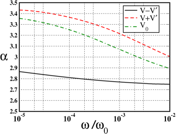
FIG. 3.: The tunneling exponent $\alpha(\omega)={\cal A}(\omega)+1$ for the models $V-V^{\prime}$, $V+V^{\prime}$, and $V_{0}$ [see Eqs. (90), (91), and (92)] at $\nu=1/2$ as a function of frequency $\omega$. The frequency is measured in units of $\omega_{0}=\kappa_{0}e^{4}$. For the model $V-V^{\prime}$ the frequency dependence of $\alpha$ is much weaker than for the models $V+V^{\prime}$ and $V_{0}$. Note that even in the latter two cases the frequency dependence is quite weak, logarithmic at most.

The model $V-V^{\prime}$ is closer to the experimental situation than other models studied in this paper, because it treats interaction as long ranged, and accounts for screening in the doped region. Thus, it is the $V-V^{\prime}$ model that is interesting to compare to experiment[5, 6, 19]. The tunneling exponent calculated above can be plotted versus $\rho_{xy}$ (see Fig. 4). Experimentally, the parameter controlling occupation of the Landau levels is the magnetic field, and so the experimentally measured $\alpha$ are shown in[5, 6, 19] as functions of $\nu^{-1}_{\rm bulk}=B/\Phi_{0}n_{\rm 2DEG}$. However, at large Hall angle, $\rho_{xx}\ll\rho_{xy}$, and away from incompressible densities, $e^{2}\rho_{xy}/h$ is quite close to $\nu^{-1}$.

Also, it would be incorrect to ignore the difference between the 2DEG density in the bulk and near the edge, and to compare the graph in Fig. 4 directly with the experimentally measured $\alpha$. One can argue (see Sec. V below) that the density near the edge exceeds $\nu_{\rm bulk}$ by $20-30\,\%$. Taking this into account, one has to rescale the slope of the experimentally observed dependence $\alpha=1/\nu_{\rm bulk}$, and to compare the curves in Fig. 3 with the dependence $\alpha=(1.2-1.3)\,\rho_{xy}e^{2}/h$. This agrees reasonably well with the average slope of the curves in Fig. 3 in the interval $1<\rho_{xy}<4$ studied experimentally[6, 19].

Of course, a more important issue is whether there are plateau-like features in the experimental dependence $\alpha(\nu)$. In the experiment[6] a straight line is observed, without any sign of plateaus. More recently, however, it was found that some samples show signs of a plateau near $\nu=1/3$. Upon rescaling of the filling factor by $1.2-1.3$, this corresponds to $\nu_{\rm edge}$ between $1/2$ and $1/3$, which is exactly where the middle of the plateau in Fig. 4 is located. However, the matter is clearly not yet resolved, and more experimental studies would be very welcome.

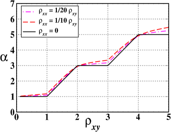
FIG. 4.: The tunneling exponent for the model $V-V^{\prime}$ [Eq.(90)] corresponding to Coulomb interaction screened by the doped region in the overgrown edge system.

There is one other type of interaction for which the problem (82) in the half plane is tractable by Fourier transform. It corresponds to the model $V+V^{\prime}$ above, defined by Eq.(91). The interaction (91) describes the situation when image charges are of the same sign as the source charges. Despite being unphysical, this problem is still worth attention, because the solution is very simple and has the behavior qualitatively different from the model $V-V^{\prime}$. Physically, this problem is similar to the one of unscreened interaction which we discuss below.

Starting with the interaction (91), one can extend the problem to the full plane, now in a symmetric way: $\Phi(x,-y)=\Phi(x,y)$, etc. Upon doing this the interaction (91) has to become unscreened, of the form $\overline{U}({\bf k})$ given by Eq.(92). Then the solution is straightforward in Fourier components:

$$\Phi_{\omega}({\bf k})=\frac{2i\chi_{\omega,k}}{|\omega|\sigma_{xx}{\bf k}^{2}+\omega^{2}/\overline{U}({\bf k})}.$$ (101)

This form automatically satisfies the boundary condition $\partial_{y}\Phi(y=0)=0$, because $\Phi$ is an even function of $y$.

The function $Q(\omega,k)$ is found by evaluating $\Phi$ at the boundary $y=0$:

$$Q^{-1}(\omega,k)=\frac{1}{\pi}\int\frac{dq}{q^{2}+k^{2}+|\omega|/\sigma_{xx}\overline{U}({\bf k})}=\frac{2}{\pi k}F(\alpha),$$ (102)

where $F(\alpha)$ is defined by Eq.(100).

Again, we now substitute this expression in Eq.(86) to calculate the instanton action. The resulting tunneling exponent $\alpha(\omega)={\cal A}(\omega)+1$ has a logarithmic frequency dependence, as shown in Fig. 3. The origin of this logarithmic dependence can be traced to the zero-bias anomaly in a diffusive conductor[26, 20]. On Fig. 5 we plot $\alpha$ as a function of $\rho_{xy}$ for several values of $\omega$. One notes that the values $\alpha$ in Fig. 5 are somewhat larger than those for the model $V-V^{\prime}$ in Fig. 4. This is due to the “antiscreening” in the model $V+V^{\prime}$ which enhances the effect of the long-range part of the interaction in the dynamics. Qualitatively, the behavior of $\alpha$ for the model $V+V^{\prime}$ is similar to that for the model $V_{0}$ discussed below.

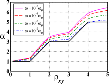
FIG. 5.: The tunneling exponent for the model $V+V^{\prime}$ [Eq. (91)] corresponding to Coulomb interaction in the presence of an “antiscreening” due to image charges in the doped region of the same sign as the source charges.

C Wiener-Hopf problem for the model $V_{0}$

Here we consider the model $V_{0}$, describing unscreened Coulomb interaction (92), i.e., in the absence of image charges of any kind. The strategy will be to derive an integral equation for $\Phi_{\omega,k}(y)$ and to deal with it using the Wiener-Hopf method. Our approach is similar to that employed by Volkov and Mikhailov in a study of the edge magnetoplasmons[27].

We start with the problem (82) written in Fourier representation with respect to $x$. Nondimensionalized, the first equation of (82) reads:

$$(k^{2}-\partial_{y}^{2})\Phi_{\omega,k}(y)+\mu n_{\omega,k}(y)=i\widetilde{\chi}_{\omega,k}\delta(y-y_{0}),$$ (103)

where $\mu=|\omega|/\sigma_{xx}$ and $\widetilde{\chi}=\chi/(|\omega|\sigma_{xx})$. As in the above discussion of the model $V-V^{\prime}$, it is convenient to place the source $\tilde{\chi}(y)$ at a small distance $y_{0}$ from the edge, and take the limit $y_{0}\to 0$ later.

Posing the correct boundary condition for Eq. (103) requires a discussion. The absence of normal current at the edge means that $\partial_{y}\Phi(y=0)=0$. On the other hand, by integrating Eq.(103) from the edge to the source $\widetilde{\chi}$, over the small interval $0\leq y\leq y_{0}$, from current conservation one obtains $\partial_{y}\Phi(y=y_{0}+0)_{y_{0}\to 0}=-i\widetilde{\chi}_{\omega,k}$. Therefore, in the limit $y_{0}\to 0$ the boundary condition is written as $\partial_{y}\Phi(y\to 0)=-i\widetilde{\chi}_{\omega,k}$. This condition defines completely the boundary value problem in the region of interest $y>y_{0}\to 0$. However, without any loss of generality, it will be convenient to assume that near the very edge, for $0<y<y_{0}$, the normal derivative $\partial_{y}\Phi$ vanishes.

Now, by performing convolution of Eq.(103) with $U_{k}(y)=\int e^{ikx}U(x,y)dx$, remembering that $n_{k}(y<0)=0$, and using the second equation of (82), we transform the problem to

  

$$\int_{y^{\prime}>0}U_{k}(y-y^{\prime})\,(k^{2}-\partial_{y^{\prime}}^{2})\Phi_{\omega,k}(y^{\prime})dy^{\prime}+\mu\Phi_{\omega,k}(y)=i\widetilde{\chi}_{\omega,k}\,U_{k}(y-y_{0})$$ (104)

We will be solving Eq. (104) in the domain $y>0$ with $k$ and $\omega$ being parameters. Hence, for simplicity, below we suppress the dependence on $\omega$ and $k$ and use $\Phi(y)$, $U(y)$, etc.

It is convenient to integrate in Eq.(104) by parts using the boundary condition $\partial_{y}\Phi(y\to 0)_{y<y_{0}}=0$, which gives:

$$(k^{2}-\partial_{y}^{2})\,\int_{y^{\prime}>0}U(y-y^{\prime})\Phi(y^{\prime})dy^{\prime}+\mu\Phi(y)=i\widetilde{\chi}U(y-y_{0})-\partial_{y}U(y)\Phi_{0},$$ (105)

   

where $\Phi_{0}=\Phi(y=0)$. The form (105) of the problem is most suitable for applying the Wiener-Hopf method to which we now proceed.

The first step is to perform Fourier expansion of $\Phi(y)$ with respect to the $y$ coordinate:

$$\Phi(y)=\sum_{q}e^{iqy}\Phi(q)$$ (106)

Since the integral in Eq.(105) is taken over $y^{\prime}>0$, in order to rewrite it in terms of $\Phi(q)$ we decompose $\Phi(y)$ as $\Phi(y)=\Phi_{>}(y)+\Phi_{<}(y)$, nonzero for $y>0$ and $y<0$, respectively. One can assume that $\Phi_{>}(y)$ and $\Phi_{<}(y)$ decay at $y\to\pm\infty$ and verify it later, when solution is found. In terms of $\Phi_{>}$ and $\Phi_{<}$, Eq. (104) becomes

  

$$\mu(\Phi_{>}(q)+\Phi_{<}(q))+(k^{2}+q^{2})U(q)\Phi_{>}(q)=iU(q)(\widetilde{\chi}\,e^{-iqy_{0}}-q\Phi_{0}).$$ (107)

   

Here the Fourier transformed interaction $U(q)$ is given by (95). In what follows we set $y_{0}=0$.

The functions $\Phi_{>}(q)$ and $\Phi_{<}(q)$ have nice analytical properties, namely, $\Phi_{<}(q)$ is an analytic function of $q$ in the upper complex half plane $\mathop{{\rm Im}}\nolimits q>0$, and $\Phi_{>}(q)$ is analytic in the lower half plane $\mathop{{\rm Im}}\nolimits q<0$. To make the discussion below more transparent, we denote $\Phi_{>}(q)$ by $\Phi_{-}(q)$, and $\Phi_{<}(q)$ by $\Phi_{+}(q)$, where $\pm$ indicate the half plane of analyticity in $q$.

Now, Eq. (107) can be written as

$$K(q)\Phi_{-}(q)+\Phi_{+}(q)=R(q),$$ (108)

where

$$K(q) = 1+\frac{1}{\mu}(k^{2}+q^{2})U(q)$$ (109)

$$R(q) = \frac{i}{\mu}U(q)\left(\widetilde{\chi}-q\Phi_{0}\right).$$ (110)

The next step is to decompose $K(q)$ into the ratio of two functions which are analytic in the upper and lower half planes, respectively:

$$K(q)=\frac{X_{+}(q)}{X_{-}(q)},$$ (111)

where

$$X_{\pm}(q)=\exp\left(\frac{1}{2\pi i}\int_{-\infty}^{\infty}{\frac{dq^{\prime}}{q^{\prime}-q\mp i0}\,\ln K(q^{\prime})}\right).$$ (112)

The asymptotic behavior of $X_{\pm}(q)$ at $|q|\gg 2\pi\kappa_{0}/\epsilon$ is $X_{+}(q)=(q+i|k|)/\lambda$, $X_{-}(q)=\lambda/(q-i|k|)$, where $\lambda=\sqrt{\mu\kappa_{0}}$.

Now, Eq. (107) turns into

$$\frac{\Phi_{+}(q)}{X_{+}(q)}+\frac{\Phi_{-}(q)}{X_{-}(q)}=\Psi(q),$$ (113)

where

$$\Psi(q)=\frac{R(q)}{X_{+}(q)}=\frac{i(\widetilde{\chi}-q\Phi_{0})}{q^{2}+k^{2}}\,\left(\frac{1}{X_{-}(q)}-\frac{1}{X_{+}(q)}\right)$$ (114)

Now we decompose $\Psi(q)$ into the sum of two functions with appropriate analytical properties:

  

$$\Psi(q)=\Psi_{+}(q)-\Psi_{-}(q)\ ;\qquad\Psi_{\pm}(q)=\frac{1}{2\pi i}\int_{-\infty}^{\infty}\frac{dq^{\prime}}{q^{\prime}-q\mp i0}\,\Psi(q).$$ (115)

The standard Wiener-Hopf reasoning[28] then leads to

$$\Phi_{+}(q)=X_{+}(q)\Psi_{+}(q)\ ;\qquad\Phi_{-}(q)=-X_{-}(q)\Psi_{-}(q).$$ (116)

Fourier transform of Eq.(116) gives $\Phi(y)$ for $y<0$ and $y>0$.

It is not difficult to find $\Psi_{\pm}(q)$ explicitly. For that, one has to substitute Eq.(114) into the Cauchy integral in Eq.(115), which gives

$$\Psi_{-}(q)=-\frac{1}{2\pi i}\int_{-\infty}^{\infty}\frac{dq^{\prime}}{q^{\prime}-q+i0}\frac{i(\widetilde{\chi}-q\Phi_{0})}{q^{2}+k^{2}}\,\left(\frac{1}{X_{-}(q)}-\frac{1}{X_{+}(q)}\right),$$ (117)

and a similar equation for $\Psi_{+}(q)$. Now, we close the integration contour in Eq.(117) in the upper or lower half plane, depending on whether $X^{-1}_{+}$ or $X^{-1}_{-}$ is to be integrated, and evaluate the integral (117) using residues. Having found $\Psi_{-}(q)$, and then using Eq.(116) to go back to $\Phi_{-}(q)$, we obtain

$$\Phi_{-}(q)=\frac{i(\widetilde{\chi}-q\Phi_{0})}{q^{2}+k^{2}}+\frac{X_{-}(q)}{2|k|}\left[\frac{1}{i|k|+q}\,\frac{\widetilde{\chi}+i|k|\Phi_{0}}{X_{-}(-i|k|)}+\frac{1}{i|k|-q}\,\frac{\widetilde{\chi}-i|k|\Phi_{0}}{X_{+}(i|k|)}\right]$$ (118)

   

Several remarks are in order about the result (118).

First of all, let us verify that $\Phi_{-}(q)$ is analytic at $\mathop{{\rm Im}}\nolimits q<0$. The expression (118) has an apparent pole in the lower half plane at $q=-i|k|$. However, it is easy to see from Eq.(118) that the residue for this pole is zero. From analyticity at $\mathop{{\rm Im}}\nolimits q<0$ it follows that $\Phi(y<0)=0$, as it should be.

Next, let us verify that the boundary value $\Phi_{0}$ is reproduced correctly. For that we expand Eq.(118) in inverse powers of $q$ at $|q|\to\infty$:

$$\Phi_{-}(q)=\frac{a}{iq}-\frac{b}{q^{2}}+...$$ (119)

Since $\Phi(y<0)=0$, one simply has $\Phi(y\to+0)=a$. To evaluate $a$, only the first term of Eq.(118) is important, because $X_{-}(q\to\infty)=\lambda/q+O(q^{-2})$, where $\lambda=\sqrt{\mu\kappa_{0}}$, and thus the second term of Eq.(118) does not contribute to $a$. From the first term one obtains $a=\Phi_{0}$, as expected.

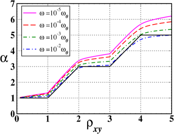
FIG. 6.: The tunneling exponent for the model $V_{0}$ (92) corresponding to unscreened Coulomb interaction. Frequency is given in units of $\omega_{0}=\kappa_{0}e^{4}$.

After these consistency checks we can proceed with finding the relation between $\Phi_{0}$ and $\widetilde{\chi}$. Conservation of current at the boundary $y=0$ for the problem (103) implies $\partial_{y}\Phi(y\to 0)=-i\widetilde{\chi}$. On the other hand, $b=\partial_{y}\Phi(y\to 0)$ in the expansion (119). By carrying out the expansion of the result (118) up to the order $q^{-2}$ to obtain $b$, and then setting up the equation $-i\widetilde{\chi}=b$, we have

$$-i\widetilde{\chi}=-i\widetilde{\chi}+\frac{1}{2\lambda|k|}\left[\frac{\widetilde{\chi}-i|k|\Phi_{0}}{X_{+}(i|k|)}-\frac{\widetilde{\chi}+i|k|\Phi_{0}}{X_{-}(-i|k|)}\right],$$ (120)

where $\lambda$ is the coefficient in the asymptotic expansion of $X_{-}(q\to\infty)$ defined above. This equation can be rewritten in the form

$$\Phi_{0}=\frac{i\widetilde{\chi}}{|k|}\,\frac{X_{+}(i|k|)-X_{-}(-i|k|)}{X_{+}(i|k|)+X_{-}(-i|k|)}.$$ (121)

According to Eq.(84), the relation (121) defines $Q(\omega,k)$ in terms of $X_{+}(i|k|)$ and $X_{-}(-i|k|)$.

The expressions for $X_{\pm}(\pm i|k|)$ can be simplified:

$$X_{\pm}(\pm i|k|)=\exp\left[\pm I(\omega,k)\right],$$ (122)

where

$$I(\omega,k)=\frac{1}{\pi}\int_{0}^{\infty}{\frac{d\xi}{\xi^{2}+1}\,\ln\left(1+\frac{1}{\mu}k^{2}(\xi^{2}+1)U(k\sqrt{\xi^{2}+1})\right)}.$$ (123)

Here $\xi=q/|k|$, $\mu=|\omega|/\sigma_{xx}$. After putting (122) into (121), one finally arrives at

$$Q(\omega,k)=|k|\coth I(\omega,k)$$ (124)

With this expression for $Q(\omega,k)$ one can go back to the effective action (85), and find the Green’s function (86) in terms of the spectral weight ${\cal A}(\omega)$ given by (88).

The integral entering Eq.(123) can easily be tabulated numerically. The spectral weight ${\cal A}(\omega)$ has a logarithmic frequency dependence, as shown in Fig. 3, similar to that of the model $V+V^{\prime}$. The behavior of the tunneling exponent $\alpha$ as a function of $\rho_{xy}$, shown in Fig. 6, is also close to that for the model $V+V^{\prime}$. One notes that the values of $\alpha$ are somewhat less than those for the model $V+V^{\prime}$ with similar parameters. This is due to a relatively weaker effect of the long-range part of the interaction in the model $V_{0}$.

V Comparison to the experiment

In this section we discuss some aspects of the overgrown cleaved edge system[5, 6, 19]. In our view, the most relevant issue concerns the 2DEG density distribution near the edge. One of the key features of cleaved edge systems is that they produce structures with supposedly an atomically sharp confining potential, and thus the 2DEG density profile near the edge is expected to be reasonably smooth. This is important in edge tunneling experiment, because the system must have a well defined filling factor even very close to the edge.

A Thomas-Fermi model

To estimate the importance of various factors controlling the density near the edge, below we consider a simplified electrostatic Thomas-Fermi model, in which the 2DEG is modeled as an ideal charge fluid, and all effects of electron-electron correlation and finite density of states are ignored, except very close to the edge. In principle, this approximation is quite reliable at distances larger than the screening length $r_{s}=\epsilon/2\pi\kappa_{0}$, and so the results will be meaningful at distances more than $r_{s}$ from the edge.

The electrostatic problem we consider involves the 2DEG density $n(x,y)$ in the half plane $y>0$, top surface charge states that are at a distance $w=600\,{\rm nm}$ above the 2DEG, a layer of charged donors parallel to the 2DEG at a distance $w_{+}=60\,{\rm nm}$ above the 2DEG plane, and also charges in the three-dimensional doped region, which in our model occupies the halfspace $y<-w_{b}$, where $w_{b}=9\,{\rm nm}$ is the width of the barrier together with the buffer region. The top surface, the 2DEG, and the doped region are assumed to be equipotentials in the problem. For simplicity, we assume that the 2DEG is grounded, and the bias voltage on the 3D doped region is very small, so that the electrochemical potentials of the two regions are essentially equal. Relative to the 2DEG, the electrostatic potential at the top surface is $V_{s}=-800\,{\rm mV}$, and the electrostatic potential at the boundary of the 3D doped region is $V_{d}\approx 20\,{\rm mV}$. (The value of $V_{d}$ reflects the chemical potential difference before the charge redistributes itself. It is given by the difference of Fermi energies in the doped region and in the 2DEG plus the confinement energy of the 2DEG.) The charge density of donors $\sigma_{+}$ is taken to be constant everywhere at $y>0$ up to the edge $y=0$. The potential $V_{d}$ is much smaller than the barrier height, which is estimated as $\simeq 120\,{\rm meV}$.

One can write down a simple analytic formula for the 2DEG density, using the electrostatic superposition principle, according to which the effects on the 2DEG due to the donors, the top surface charge, and the doped region, can be treated separately and then added.

First, let us consider the charge induced by donors, when the top surface and the doped region are at the same electrostatic potential as the 2DEG. We make an approximation $w\gg w_{+}$, which allows us to move the top surface to infinity, and thus to ignore it. Also, we assume that the distance to the doped region $w_{b}\ll w_{+}$, the separation of the donors from the 2DEG. With the values for $w$, $w_{+}$, and $w_{b}$ quoted above, both approximations are reasonable. The resulting contribution to the 2DEG charge density is

$$\sigma^{(1)}_{\rm 2DEG}(y)=\frac{2\sigma_{+}}{\pi}\,\arctan\,\frac{y}{w_{+}}.$$ (125)

It describes the 2DEG density, constant and equal to $\sigma_{+}$ at $y\gg w_{+}$, and decreasing to $0$ near the edge.

The effect of the top surface potential $V_{s}$, in the absence of donors, and with the 2DEG and the doped region at zero electrostatic potential, can be evaluated as follows. In the approximation $w_{b}\ll w$, the problem is equivalent to the standard electrostatic problem of a half-open slit, with one side of the slit being at the potential $V_{s}$ with respect to the other side and the end. The induced charge density in this problem is

$$\sigma^{(2)}_{\rm 2DEG}(y)=\frac{\epsilon V_{s}}{4\pi w}\,\tanh\,\frac{\pi y}{2w}.$$ (126)

This contribution is constant and equal to $\epsilon V_{s}/4\pi w$ in the bulk, at $y\gg w/\pi$, and decreases to zero near the edge.

Finally, the effect of potential difference between the 2DEG and the doped region can be considered ignoring the top surface and the donors. The relevant spatial scale in this case is $w_{b}\ll w_{+},w$, and so the problem is reduced to that of a ground half plane (representing the 2DEG), and a conducting plane perpendicular to it, at a relative potential $V_{d}$, located a distance $w_{b}$ away from the ground half plane. The charge density induced in the 2DEG is

$$\sigma^{(3)}_{\rm 2DEG}(y)=\frac{\epsilon V_{d}}{2\pi^{2}}\,\frac{1}{\sqrt{(y+w_{b})^{2}-w_{b}^{2}}}.$$ (127)

It behaves as $1/y$ away from the edge, and as $1/\sqrt{y}$ near the edge. The square root divergence near the edge is an artifact of the simplified model ignoring finite density of states of the 2DEG. In a Thomas-Fermi model, the divergence would be cut at a distance $\sim r_{s}$ from the edge.

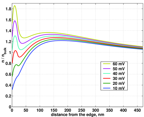
FIG. 7.: Density distribution in the 2DEG near the edge plotted for six values of the potential $V_{d}$ of the doped region (listed from top to bottom). The top surface potential $V_{s}=-800\,{\rm mV}$ and the donor density $\sigma_{+}=1.94\cdot 10^{11}\,{\rm cm}^{-2}$ correspond to the 2DEG bulk density $n_{\rm bulk}=10^{11}\,{\rm cm}^{-2}$. The geometrical parameters used are defined in the text.

The resulting 2DEG charge density is a sum of three terms, $\sigma_{\rm total}=\sigma^{(1)}_{\rm 2DEG}+\sigma^{(2)}_{\rm 2DEG}+\sigma^{(3)}_{\rm 2DEG}$. To eliminate the unphysical singularity near the edge due to $\sigma^{(3)}$, we average the density $\sigma_{\rm total}$ over intervals of length $2r_{s}$, and consider

$$\sigma_{\rm total}^{\rm av}(y)=(2r_{s})^{-1}\int^{y+r_{s}}_{y-r_{s}}\sigma_{\rm total}(y^{\prime})dy^{\prime}.$$ (128)

The averaged density $\sigma_{\rm total}^{\rm ave}$ is plotted in Fig. 7 for several values of the doped region potential $V_{d}$. The screening radius used in the averaging is taken to be $r_{s}=20\,{\rm nm}$.

One can see from Fig. 7 that the density within $\simeq 200\,{\rm nm}$ near the edge is quite sensitive to the potential $V_{d}$. Another feature evident in Fig. 7 is that the density close to the edge exceeds that in the bulk by $20-30\,\%$. The 2DEG density approaches the bulk value at distances $\geq 400\,{\rm nm}$ from the edge. Also, there is a peak in the density profile near the very edge, resulting from the $\sigma^{(3)}$ contribution averaged over the length $\simeq r_{s}$. This peak makes the density profile nonmonotonic, with a minimum at $\simeq 30-40\,{\rm nm}$ from the edge. Altogether, the 2DEG density near the edge is smooth but not perfectly uniform.

It should be remarked that our simplified electrostatic model is perhaps insufficient at distances smaller than or of the order of $r_{s}\simeq 20\,{\rm nm}$. Thus the smallest scale features in Fig. 7, such as the density peak near the edge, should be taken with caution. Moreover, we used the Thomas-Fermi model, the screening radius $r_{s}$, etc., in the absence of magnetic field. It remains to be seen whether the results are preserved in a more accurate treatment accounting for Landau levels, finite 2DEG compressibility, and exchange effects. On the other hand, on spatial scales larger than $r_{s}$, the results obtained from a purely electrostatic model should be reliable.

One issue that can be addressed using the electrostatic model is the calibration of density in the experiment [5, 6]. The tunneling exponent $\alpha$ is presented there as a function of magnetic field, which is calibrated in terms of the bulk filling factor using magnetotransport data. However, the filling factor relevant for tunneling is that near the edge. According to the above, in the region 100 $\sim$ 300 nm from the edge, the density is at least $20-30\%$ higher than in the bulk. If one assumes that this is the relevant distance scale for charge relaxation at the temperatures and voltages employed in the experiments, then the dependence $\alpha=1/\nu_{\rm bulk}$ observed in [6, 19] translates into $\alpha\approx(1.2-1.3)\,\nu^{-1}_{\rm edge}$. In actuality, the relevant distance scale will depend on the filling factor and the cleanliness of the edge, as well as the energy of the tunneling electron.

One notes that after accounting for the difference between $\nu_{\rm edge}$ and $\nu_{\rm bulk}$ the dependence $\alpha(\nu)$ shifts closer to the theoretical curves (see Fig. 8).

B Two-mode model

Because the 2DEG density profile discussed above is significantly nonmonotonic near the edge, it is possible that this may change the structure of the edge modes. More precisely, suppose that the peak density near the edge is so high that the filling factor reaches $\nu=1$ within the region $\simeq 30\,{\rm nm}$ corresponding to the peak displayed in Fig. 7. Then the edge mode on the periphery will correspond to $\nu=1$ even when $\nu<1$ away from the edge. In this case, in addition, there will also be counterpropagating modes positioned on the inner side of the incompressible $\nu=1$ region. The number of these modes and their Hamiltonian will depend on $\nu$ somewhat away from the edge. This type of acomposite structure of the edge was first proposed by MacDonald for the $\nu=2/3$ system, based on a Hartree-Fock analysis[29].

In this model, the tunneling electron is injected into the outer $\nu=1$ mode, because of higher overlap of the tunneling state with the mode closest to the edge. We assume that the edge is so clean that we can neglect scattering between different edge modes. Then, the inner modes will be important only to the extent that tunneling charge couples with them by Coulomb interaction, and shakes them up. In this scenario, after tunneling there is no statistics change of the injected particle, since it remains in the fermionic $\nu=1$ edge state. Therefore, one expects a smooth dependence of the tunneling exponent on $\nu$, without any cusps or plateaus.

To estimate the shakeup effect due to Coulomb coupling to the inner modes, let us represent them by a single charged mode. Thus the system can be described by two counterpropagating chiral modes:

  

$${\cal S}=\frac{1}{2}\sum\limits_{\omega,k}\left(i\omega k\,\left(\phi^{(1)}\phi^{(1)}-g\phi^{(2)}\phi^{(2)}\right)+\omega^{2}\sum\limits_{i,j=1,2}V_{ij}\phi^{(i)}\phi^{(j)}\right)+\phi^{(1)}J,$$ (129)

   

where $g=1-\nu$ and $V_{ij}$ is the coupling matrix, expressed in terms of the interactions $V_{ij}^{0}$ as follows: $V_{11}=V_{11}^{0}$, $V_{12}=gV_{12}^{0}$, $V_{21}=gV_{21}^{0}$, $V_{22}=g^{2}V_{22}^{0}$. The form of the action (129) can easily be justified in the same way as in Sec. III. In this case there is no issue of charge injection in the inner mode, and so there are no complications related with counterterms, as in (44).

It is straightforward to write down the Green’s function by evaluating the saddle point of the quadratic action (129). The result reads

  

$$G(\tau)=\exp\left(-\frac{1}{8\pi^{2}}\int\frac{(\omega^{2}V_{22}-ig\omega k)|J_{\omega}|^{2}\,d\omega\,dk}{(\omega^{2}V_{11}+i\omega k)(\omega^{2}V_{22}-ig\omega k)-\omega^{4}V_{12}V_{21}}\right)$$ (130)

   

To evaluate the Green’s function, we assume that the coupling matrix $V_{ij}$ has no $k$ dependence. This is true for the screened Coulomb interaction $2\pi e^{2}(1-e^{-2a|k|})/\epsilon|k|$ at $a|k|\leq 1$, where $a$ is the distance from the edge mode location to the doped region. Hence the length $a$ is somewhat larger than the barrier width $w_{b}$.

In this case the integral over $k$ can be done by residues, and the result is $G(\tau)=\tau^{-\alpha}$, where

$$\alpha=\frac{V_{11}^{0}+gV_{22}^{0}}{\sqrt{(V_{11}^{0}+gV_{22}^{0})^{2}-4gV_{12}^{0}V_{21}^{0}}}$$ (131)

The dependence $\alpha(\nu)$ in the interval $0<\nu<1$ is smooth, without singularities, as it should be in the case when the effect of the fractional edge is purely a shakeup, not accompanied by injection of charge.

To estimate numerical values of $\alpha$, we consider a model in which the interactions $V_{ij}^{(0)}$ are given by the Coulomb potential screened by the doped region. We assume that the outer edge is separated from the doped region by a barrier of thickness $w$, and the inner and outer edge states are a distance $a$ apart. Then

  

$$V_{11}^{(0)}=\frac{2\pi e^{2}}{\epsilon|k|}(1-e^{-2w|k|}),\qquad V_{22}^{(0)}=\frac{2\pi e^{2}}{\epsilon|k|}(1-e^{-2(w+a)|k|}),\qquad V_{12}^{(0)}=V_{21}^{(0)}=\frac{2\pi e^{2}}{\epsilon|k|}e^{-a|k|}(1-e^{-2w|k|})$$ (132)

   

We consider the limit of small $k$, where the interactions $V_{ij}^{(0)}$ do not depend on $k$: $V_{11}^{(0)}=2w(2\pi e^{2}/\epsilon)$, $V_{22}^{(0)}=2(w+a)(2\pi e^{2}/\epsilon)$, $V_{12}^{(0)}=V_{21}^{(0)}=(2w-a)(2\pi e^{2}/\epsilon)$.

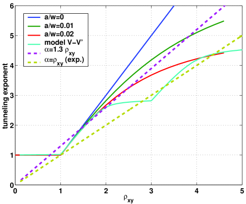
FIG. 8.: Solid curves:  The tunneling exponent in the composite edge model (129) is shown for three values of the ratio $a/w$ of the distance between the outer and inner edges and the tunneling barrier width. For comparison, a theoretical curve for the $V-V^{\prime}$ model is shown, for $\rho_{xx}=\rho_{xy}/10$ and $\omega=10^{-5}\kappa_{0}e^{4}$. Dashed curves:  The straight line $\alpha=\rho_{xy}$ corresponds to experiment (Refs. [5, 6, 19]), and the line $\alpha=1.3\rho_{xy}$ is obtained by correcting the filling factor by the ratio of the densities near the edge and in the bulk.

In this model, the only parameter is the ratio $a/w$. The tunneling exponent is plotted in Fig. 8 as a function of $\rho_{xy}=\nu^{-1}$ for several values of $a/w$. On the same figure, we show the experimental dependence of $\alpha$ versus $\rho_{xy}$ rescaled by a factor $1.3$ as discussed above.

The distinct feature of the composite edge model is the absence of plateaus in the tunneling exponent $\alpha(\nu)$. However, note that in order for the tunneling exponent $\alpha$ to fall in the right range, one has to assume unphysically small values of the ratio $a/w$. Also, the theoretical curves for nonzero $a/w$ have curvature which is absent in the experimental curve. This curvature is even more significant at higher values of the parameter $a/w$ and is unlikely to disappear if one takes into account possible dependence of $a/w$ on $\nu$. It is apparent that this simplified two-mode model does not agree with the experimental results on tunneling. Nevertheless, it illustrates the point that, if scattering between edge modes is sufficiently small, a complicated edge structure can lead to large changes in the observed tunneling exponent, which will not be closely related to the bulk filling factor.

VI Summary

The problem of tunneling into the edge of a composite fermion QH system is treated for long-range Coulomb interaction between electrons, as well as for a short-range interaction model. It is shown that in the case of diffusive CF dynamics described by finite $\rho_{xx}$, the tunneling exponent is controlled by the coupling of tunneling electron to the charged edge mode. The effective action for this mode is a generalized chiral Luttinger action with a nonlocal dissipative term.

The tunneling exponent is found to be a continuous and monotonic function of $\rho_{xy}$, given, in the limit $\rho_{xx}\to 0$, by $\alpha=1+\frac{e^{2}}{h}(\rho_{xy}-|\rho^{(0)}_{xy}|)$, where $\rho^{(0)}_{xy}$ is the CF Hall resistivity due to motion in the residual magnetic field. In order to verify the robustness of the results we consider several models for the electron-electron interaction: the short-range and Coulomb interaction, and, in the latter case, with and without electrostatic screening due to image charges in the doped region.

The dependence of $\alpha$ on $\rho_{xy}$ is characterized by plateaulike features, not observed in the experiments on cleaved edge systems. We discuss the 2DEG density profile near the cleaved edge, and propose that the discrepancy between theory and experiment is possibly due to spatial variation of the density near the edge and, in particular, to a nonmonotonic density profile, giving rise to a composite structure of edge modes.

Acknowledgments:
We are grateful to Albert Chang and Matt Grayson for many useful discussions and for sharing their data prior to publication. We thank Bell Labs for support and hospitality at the initial stage of this project. This work was supported in part by the MRSEC Program of the NSF under Grant No. DMR 98-08941 and by NSF Grant No. DMR 99-81283.

A Estimate for the ballistic regime

In the ballistic regime, for length scales smaller than the composite fermion mean free path $l$, the conductivity tensor is nonlocal in space. Close to the edge, the CF conductivity $\sigma^{(0)}_{\alpha\beta}(\bf{r},\bf{r^{\prime}},\omega)$ depends on the distance from the edge, as well as on the separation $\bf{r}-\bf{r^{\prime}}$. As a crude approximation, however, in order to estimate the contribution of the short-distance response to the tunneling exponent, we shall ignore the dependence on the distance from the edge and use, instead, the bulk CF conductivity, which depends only on $\bf{r}-\bf{r^{\prime}}$ [25].

As discussed in Secs. II and III, for a nonlocal conductivity we may still approximate the Green’s function $G(\tau)$ using the factorization (68), but the actions $S(\tau)$ and $S_{\rm free}(\tau)$ should be evaluated using the correct nonlocal conductivity. Instead of this, in our approximation, we use the form (70) for ${\cal S}$, with the change that we replace the macroscopic conductivity $\sigma_{xx}$ by the quantity $\sigma_{l}(|k|)$, which is the wave-vector dependent longitudinal conductivity for the bulk compressible Hall state. Specifically, at $\nu=1/2$, according to Ref.[7], we have

$$\sigma_{l}(k)\sim(e^{2}/8\pi\hbar)(k/k_{F}),$$ (A1)

for $l^{-1}<k<k_{F}$, while $\sigma_{l}(k)$ reduces to the macroscopic conductivity $\sigma_{xx}$ for $k<l^{-1}$. We continue to approximate the Hall conductivity in Eq.(70) by its macroscopic value $\sigma_{xy}$.

In evaluating Eq.(70), it is convenient to combine contributions from wave vectors $k$ and $-k$, and replace the sum over $k$ by an integral over positive values of $k$. If the frequency $\omega$ is sufficiently small, there will be two distinct regions which can contribute significantly to the integral. The first, for $k<l^{-1}$, gives the same contribution as was found in Sec. III above, since $\sigma_{l}(k)=\sigma_{xx}$ in this region. In the region $k>l^{-1}$, we may set $q=k$, when $\omega$ is sufficiently small, so that the integrand takes the form

$$I_{\rm largek}={|J(\omega)|^{2}\over|\omega||k|\sigma_{xy}}{\rm Re}{\sigma_{xy}\over(\sigma_{l}(k)+i\sigma_{xy})}.$$ (A2)

.

The last factor in Eq.(A2) is small for $k\ll k_{F}$ but becomes of order unity for $k\approx k_{F}$, where $\sigma_{l}(k)\approx\sigma_{xy}$. The contribution from this region to the integral could therefore make a contribution of order unity to the tunneling exponent $\alpha$. However, this contribution may be largely or completely canceled by the corresponding contribution to $S_{\rm free}$.

If we neglect the difference between the longitudinal and transverse conductivities at the finite wave vector $k$, then

$${\rm Re}{1\over(\sigma_{l}(k)+i\sigma_{xy})}=\rho_{l}(k)$$ (A3)

which is the longitudinal resistivity at wave vector $k$. In calculating $S_{\rm free}$, using the same assumptions, we obtain the identical expression, because the longitudinal conductivity of the composite fermions is the same as that of the electrons. Thus the contribution to the tunneling exponent from short wavelengths is canceled, in this approximation. We therefore wind up with the same value for $\alpha$ as was obtained in Sec. III, namely $\alpha\sim 3$ at $\nu=1/2$, for a system where $\sigma_{xx}\ll\sigma_{xy}$.

It is not possible to say whether a similar cancelation would occur in a proper analysis incorporating the nonlocal conductivity. If the cancellation does not occur, then the surviving contribution from short wavelengths could give a contribution of order unity to the tunneling exponent, which would be independent of the mean-free-path in the limit $l\ll k_{F}^{-1}$.

REFERENCES

- [1] X.-G. Wen, Int. J. of Mod. Phys. B6, 1711 (1992); Phys. Rev. Lett. 64, 2206 (1990); Phys. Rev. B43, 11025 (1991); Phys. Rev. B44, 5708 (1991);
- [2] C.L. Kane, M.P.A. Fisher and J. Polchinski, Phys. Rev. Lett. 72, 4129 (1994); C.L. Kane and M.P.A. Fisher, Phys. Rev. B51, 13449 (1995)
- [3] F.P. Milliken, C.P. Umbach, and R.A. Webb, Solid State Comm. 97, 309 (1996);
- [4] L.N. Pfeiffer, K. W. West, H. L. Stormer, J. P. Eisenstein, K. W. Baldwin, D. Gershoni, and J. Spector, Appl. Phys. Lett. 56, 1697 (1990)
- [5] A.M. Chang, L.N. Pfeiffer, and K.W. West, Phys. Rev. Lett. 77, 2538 (1996)
- [6] M. Grayson, D.C. Tsui, L.N. Pfeiffer, K.W. West, and A.M. Chang, Phys. Rev. Lett. 80, 1062 (1998)
- [7] B.I. Halperin, P.A. Lee, N. Read, Phys. Rev. B47, 7312 (1993)
- [8] J. K. Jain, Phys. Rev. Lett. 63, 199 (1989).
- [9] D.B. Chklovskii, Phys. Rev. B51, 9895 (1995); L. Brey, Phys. Rev. B50, 11861 (1994)
- [10] A.V. Shytov, L.S. Levitov, B.I. Halperin, Phys. Rev. Lett., 80, 141 (1998)
- [11] S. Conti and G. Vignale, J. Phys. - Condens. Mat. 10: (50) L779-L786 (1998)
-
[12]
J.H. Han and D.J. Thouless,
Phys. Rev. B, 55, 1926 (1997);
J. H. Han, Phys. Rev. B, 56, 15806 (1997) - [13] U. Zülicke and A.H. MacDonald, Phys. Rev. B60, p. 1837 (1999)
- [14] A.M.M. Pruisken, B. Skoric, M.A. Baranov, Phys. Rev. B60, p. 16838 (1999)
- [15] A. Alekseev, V. Cheianov, A.P. Dmitriev, V.Yu. Kachorovskii, Pis’ma Zh. Éksp. Teor. Fiz 72 (6), 481-486 (2000) [JETP Lett. 72 (6), 333-336 (2000)]; cond-mat/9904076
- [16] A. Lopez and E. Fradkin, Phys.Rev.B59, 15323 (1999)
- [17] D.-H. Lee, X.-G. Wen, Edge tunneling in fractional quantum Hall regime, cond-mat/9809160
- [18] D.V. Khveshchenko, Solid State Commun. 111: (9), 501-505 (1999); cond-mat/9806270
- [19] A.M. Chang, M.K. Wu, C.C. Chi, L.N. Pfeiffer, K.W. West, Phys. Rev. Lett. 86, 143 (2000)
-
[20]
L.S. Levitov, A.V. Shytov,
Pis’ma Zh. Éksp. Teor. Fiz 60 (3), 200-205 (1997)
[JETP Lett. 66, 214 (1997)];
also, in: Correlated Fermions and Transport in Mesoscopic Systems, edited by T. Martin, G. Montambaux, and J. Tran Thanh Van (Editions Frontieres, 1996), p. 513 - [21] L.D. Landau and E.M. Lifshits, Statistical Physics, Part I, Ch. XII, § 125, p.389 (Pergamon Press, 1982)
- [22] S. He, P.M. Platzman, B.I. Halperin, Phys. Rev. Lett. 71, 777 (1993)
- [23] Y.B. Kim, X.-G. Wen, Phys. Rev. B50, 8078 (1994)
- [24] A.V. Shytov, Ph. D. Thesis, L.D. Landau Institute for Theoretical Physics, Chernogolovka, 1999
- [25] In Ref.[18], Khveshchenko carried out an approximate calculation in which he considered, simultaneously, effects of an unscreened Coulomb interaction and a nonlocal CF conductivity, on the charge spreading action and the curve for , above the CF scattering frequency. We have not been able to make a direct comparison of our results with his, however. We note that Khveshchenko does not include a term in the action which correspond to the logarithm of the free-fermion Green’s function, nor does he subtract a term corresponding to .
- [26] B.L. Altshuler, A.G. Aronov, P.A. Lee, Phys.Rev.Lett. 44, 1288 (1980)
- [27] V.A. Volkov and S.A. Mikhailov, Zh. Éksp. Teor. Fiz 94 (8), 214-241 (1988) [Sov. Phys. JETP 67 1639 (1988)]
- [28] B. Noble, Methods based on the Wiener-Hopf technique, (Pergamon Press, London, 1958)
-
[29]
A.H. MacDonald, Phys.Rev.Lett. 64, 222 (1990);
M.D. Johnson and A.H. MacDonald, Phys.Rev.Lett. 67, 2060 (1991) -
[30]
B.L. Altshuler, L.B. Ioffe, and A.J. Millis,
Phys. Rev. B50, 14049 (1994);
Y.B. Kim, A. Furusaki, X.-G. Wen and P.A. Lee, Phys. Rev. B50, 17917 (1994)