Synchronization, Diversity, and Topology of Networks of Integrate and Fire Oscillators.

Abstract

We study synchronization dynamics of a population of pulse-coupled oscillators. In particular, we focus our attention in the interplay between networks topological disorder and its synchronization features. Firstly, we analyze synchronization time $T$ in random networks, and find a scaling law which relates $T$ to networks connectivity. Then, we carry on comparing synchronization time for several other topological configurations, characterized by a different degree of randomness. The analysis shows that regular lattices perform better than any other disordered network. The fact can be understood by considering the variability in the number of links between two adjacent neighbors. This phenomenon is equivalent to have a non-random topology with a distribution of interactions and it can be removed by an adequate local normalization of the couplings.

I Introduction

Synchronization of populations of interacting oscillatory units takes place in several physical, chemical, biological and even social systems[1, 2, 3]. Networks of interacting oscillators are currently used to modelize these phenomena. In this paper we will focus on a special kind of interacting oscillators, namely pulse coupled oscillators. These units oscillate periodically in time and interact, each time they complete an oscillation, with its coupled neighbors sending them pulses which modify their current states. These systems show a rich spectrum of possible behaviors which ranges from global synchronization[4] or spatio-temporal pattern formation[5, 6] to self-organized criticality[7]. Although some theoretical approaches have been proposed, in general, the singular nature of pulse-like interactions does not allow to describe the system in terms of tractable differential equations. Despite this, some methods have been developed to find the attractors of the dynamics and study their relative stability[4, 8, 5].

In this paper, we want to focus on the effects that different topologies have on the dynamical properties of the network. In particular, we will study how does network’s topology affect global synchronization. So far, most of the studies on networks of coupled oscillators have been done on either small connectivity lattices (usually 1D rings)[8, 5] or globally coupled networks (all to all coupling)[4]. Nevertheless, there is some work done in networks of continuously coupled oscillators (Kuramoto’s)[9, 10, 11] and Hodgkin-Huxley neuron-like models[12] where different non-standard topologies are considered. Among these, the so-called Small-world networks seem to be an optimal arquitecture, in terms of activity coherence, for some of these coupled systems[11, 13].

Pulse coupled oscillators are commonly used to modelize driven biological units such as pacemaker cells of the heart[14] and some types of neurons[15]. In these systems, synchronization is usually considered to be a relevant state. Regarding heart, pacemakers must be synchronized in order to give the correct heart rhythm avoiding arrhythmias or other perturbed states. In populations of neurons, synchronization has been experimentally reported[16] and is believed to play a role in information codification[17]. Therefore, it is interesting to check which kind of topologies makes the network reach a coherent state more easily and uncover why is it so by looking for its responsible mechanisms. We will focus in a whole family of networks which are characterized by its increasing degree of disorder, i.e. ranging from regular lattices to completely random networks.

The structure of this paper is the following. In Sec. II we introduce the model of pulse-coupled oscillators which is going to be used throughout the paper. In Sec. III we start studying synchronization of populations of these coupled oscillators in random networks. In Sec. IV we compare random network performance with the more classical regular lattices. In Sec. V we consider a more general family of networks with a variable degree of randomness and study its synchronization properties. Moreover, the interplay between diversity, interaction and topology is also discussed. In the final Section we present our conclusions.

II Basics

We study the synchronization of a network of $N$ oscillators interacting via pulses. The phase of each oscillator $\phi_{i}$ evolves linearly in time

$$\frac{d\phi_{i}}{dt}=1\hskip 20.00003pt\forall i=1,\ldots,N$$ (1)

until one of them reaches the threshold value $\phi_{th}=1$. When this happens the oscillator fires and changes the state of all its vicinity according to

$\displaystyle\phi_{i}\geq 1\Rightarrow\left\{\begin{array}[]{l}\phi_{i}\rightarrow 0\\ \phi_{j}\rightarrow\phi_{j}+\Delta(\phi_{j})\end{array}\right.,$

where $j\subset\Gamma(i)$, $\Gamma(i)$ being the list of nearest neighbors of oscillator $i$. The nonlinear interaction is introduced in the Phase Response Curve (PRC) $\Delta(\phi)$. We use a PRC which induces a global synchronization $(\phi_{1}=\phi_{2}=...=\phi_{N})$ of the population of oscillators: $\Delta(\phi)=\varepsilon\phi$ with $\varepsilon>0$ . This PRC is, indeed, the most simple type of interaction that always leads to a synchronizated state whatever the initial conditions are. In other words, synchronization is the unique attractor of the dynamics. Altough it has only been mathematically proved for all-to-all[4] and local[8] couplings, for all the topologies we have dealt with, synchronization holds. Therefore the dynamics could also be expressed as

$$\frac{d\phi_{i}}{dt}=1+\varepsilon\sum_{j\subset\Gamma(i)}\delta(t-t_{j}),$$ (2)

where $t_{j}$ are the firing times of $\phi_{j}$. To define a certain degree of synchronization in our simulations, we define the variable

$$m\equiv\frac{1}{N}\sum_{i=1}^{N}(1-\phi_{i}(t_{1}^{+}))$$ (3)

measured each time $\phi_{1}=0$. The choice of oscillator $1$ as a reference is completely arbitrary. Notice that measuring the phases at $t_{1}^{+}$ ensures that these phases are $0$ if they are synchronized with oscillator $1$, not depending on the order they fire. In this way, we have a series of system “snap-shots” which mathematically correspond to a return map of the dynamics (see Fig. 1). Synchronization time $T$ is thus defined as the time needed to reach $m=1$. When this happens, all oscillators will always fire in unison.

FIG. 1.: Typical evolution of $m$. The activity coherence of the system increases with time. At time $T$ the population reaches global synchronization ($m(t=T)=1$). In this example, we consider a population of $N=300$ oscillators with arbitrary initial conditions ($m(t=0)\sim 0.5$).

III Random networks

We start studying synchronization of a population of coupled oscillators by defining a Random Network ($RN$). We restrict ourselves to the most simple type of $RN$ [19], that is, we randomly select a pair of the $N$ nodes and establish a link among them, repeating this procedure up to a certain number of links $l$. Notice that, with this wiring method, there is no guarantee of ending up with a connected network (where there must be a path connecting any pair of nodes). Dealing with a network splitted into two or more clusters would make global synchronization ($m=1$) impossible so we should avoid such pathological configurations. In order to have a connected network one has to work over a threshold number of links which ensures connectivity [20]

$$l\gg\frac{N}{2}\ln(N).$$ (4)

Therefore we can study RN whose number of links $l$ runs from the above limit up to the globally connected network (all to all coupling) which has $l=N(N-1)/2$. In addition, if we want to study the transient to synchronization, one should always stay in the limit

$$N\varepsilon\ll 1,$$ (5)

otherwise synchronization would be achieved in a few firings due to the stronger interaction.

As one expects, when the number of links $l$ is increased, the time needed to reach synchronization $T$ diminishes, having its lowest value for the globally connected case. What is really interesting is how does $T$ decrease as we consider networks with more links. It turns out that $T$ follows a power-law with a slope which is independent of the number of nodes.

$$T\sim l^{-\alpha}\hskip 20.00003pt\forall N,$$ (6)

with $\alpha=1.30\pm 0.05$ for $\varepsilon=0.01$. In Fig. 2 this behavior is shown. In these simulation results, each point is averaged over different random topologies with the same number of links and over different initial arbitrary conditions for all the oscillators.

FIG. 2.: $T$ as a function of $l$ for a fixed number of oscillators $N$ and fixed interaction strength $\varepsilon=0.01$. Results are averaged over 100 different arbitrary initial conditions in 10 different random topologies. The lowest value of $l$ is in each case the one which statistically guarantees that the network is connected and the highest one is all-to-all coupling. For higher values of $N$ the power-law behavior is lost since relation (3) does not hold anymore.

In addition, one can study how does $T$ increase with the number of oscillators $N$. We find that it also follows a power-law behaviour which does not depend on the number of links $l$ considered

$$T\sim N^{\beta}\hskip 20.00003pt\forall l,$$ (7)

with $\beta=1.50\pm 0.05$ for $\varepsilon=0.01$. Therefore, once the interaction strength is set, we can characterize synchronization time $T$ by means of network’s geometrical properties trough the scaling relation

$$T\sim\frac{N^{\beta}}{l^{\alpha}}.$$ (8)

which can be rewritten as

$$\frac{T}{N^{2\alpha-\beta}}\sim\left(\frac{l}{N^{2}}\right)^{\alpha},$$ (9)

In Fig. 3 we plot the collapse of data curves according to Eq. 9 and the agreement is excellent. The exponents $\alpha$ and $\beta$ are constant within the error bars for the checked values of $\varepsilon$ ($0.1>\varepsilon>0.005$).

FIG. 3.: Collapse of data curves $T(l,N)$ supporting the scaling hypothesis $T\sim N^{\beta}l^{-\alpha}$ for $\varepsilon=0.01$.

IV Random Networks versus Regular Lattices

Once we have seen the synchronization features of RN, it would be interesting to compare them with the performance of Regular Lattices ($RL$). In the 1D RL we consider, each oscillator is coupled to its $2l/N$ nearest-neighbors in a ring-like (1D reticle with periodic boundary conditions) network. In Fig. 5 there is an example of $RL$ with $2l/N=4$. In order to do the comparison we must calculate $T$ for the $RL$, always keeping the same number of nodes and links as in the RN cases. Since the $RL$ is the topological configuration which is a connected network with a minimum number of links ($l=N$) we can also explore topologies with fewer links than the $RN$.

Another point one has to take into account when studying $RL$ with a growing number of links $l$ is that it is not possible to add just one link to pass from one configuration to another since it would break the regularity of the lattice. Instead, one has to work with integer values of $2l/N$, that is, adding a next nearest neighbor to all oscillators when passing from one configuration to the next one that have more links. Therefore, altough we can start from an initial minimal configuration with less links, we have less points to study.

In Fig. 4 results for $\varepsilon=0.01$ are shown. One can clearly see that the $RL$ performs better than the $RN$ for all degrees of connectivity. This result holds for all $\varepsilon>0$. Nevertheless, this difference is only appreciable for lower values of $l$ so that as our network has more links it quickly vanishes. When we are close to the globally connected network, the synchronization features of both kind of networks are roughly the same, while in the low connectivity case, the $RN$ has synchronization time $T$ much longer (about twice) than the $RL$.

FIG. 4.: $T$ as a function of $l$ with a fixed number of oscillators $N=100$ and interaction strength $\varepsilon=0.01$ for the two kind of extreme networks $RL$ and $RN$. $RL$ always performs better than $RN$ although its difference quickly vanishes as we tend to a globally coupled network.

V Mixed Topologies

So far, we have checked the synchronization features of the two extreme kind of networks: RN and the RL. Nevertheless, there exists a whole family of networks that lie between these two limits. They are networks of mixed nature, that is, although they may have some random connections, also posses an underlying regular structure. Recently, this kind of networks have received a lot of attention [11, 13, 22], specially due to to the so-called Small-world networks. These networks, basically a regular lattice with a very small amount of random connections, have the advantage of having a low average distance among nodes while keeping a highly clustered structure. In this work, we examine synchronization time for networks with all degree of randomness ranging from the RL to RN.

We parametrically characterize these networks with a re-wiring probability per link $p$. It defines the following randomization procedure: starting from an initial RL of $l$ links, we cut each link with probability $p$ and re-wire it between two randomly chosen pair of nodes. Notice that our method slightly differs from other used by some authors who just rewire one edge of the link [13] or add new ones[21]. In this way, we keep the number of links $l$ constant and recover the previous two limiting cases, the $RN$ and the $RL$, for $p=1$ and $p=0$ respectively (see Fig. 5).

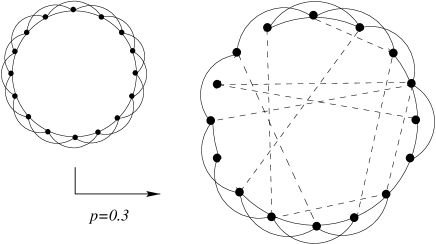
FIG. 5.: Randomization procedure for an initial RL with links to first and second nearest neighbors. Each links is cut with a probability $p=0.3$ and re-wired between two randomly selected pair of nodes (dashed lines). For $p=0$ we have again the $RL$ since no link is re-wired while for $p=1$ the pure RN is recovered.

In Fig. 6 we see the synchronization time $T$ for a network of $N=300$ oscillators with $2l/N=16$. One can clearly see that $T$ grows monotonously as we introduce more disorder into the system (increasing $p$). For different $N$ and $l$ the behavior of $T$ is qualitatively the same.

FIG. 6.: Synchronization Time $T$ for the whole range of re-wiring probability $p$. Each point is averaged over 1000 realizations for a system of $N=300$ oscillators and $2l/N=16$. $T$ increases monotonously with $p$ as the dispersion in the number of links also does. This figure can be thought as a cross section of Fig. 4, with an extra p-axe. Empty circles correspond to the normal case. Filled squares show the results once the interactions have been normalized according to Eq. 10.

These results obviously raise a question: why does topological disorder slow the synchronization process?. The re-wiring process induces a random distribution of links for any oscillator. Therefore, two adjacent units can have a very different number of oscillators. This fact is crucial since the incoming signal from the firings of the neighborhood of a given oscillator can be much larger or smaller than the signal that another of its neighbors receive. In this case, the two oscillators have different effective frequencies. The larger the difference in their effective driving, the more difficult is to synchronize these two units. This can be thought as a kind of dynamic frustation among two adjacent oscillators. One way of quantifying this problem is to check the variability in the number of neighbours per oscillator. In Fig. 7 we can see how does the dispersion in the number of links per node grow as we induce more topological disorder. This dispersion $\sigma^{2}$ is zero for $p=0$ ($RL$) whereas for a $p=1$ ($RN$) the distribution of links is known to follow a Poisson distribution with a variance equal to $2l/N$ when $N\rightarrow\infty$ [19]. As we can see, both Fig. 6 and 7 look quite similar, they show a monotonic growth with the re-wiring probability $p$ wich seem to saturate for values close to $1$.

FIG. 7.: Dispersion ($\sigma^{2}$) in the number of links for the whole range of p. Each point corresponds to an average of 1000 realizations for a system of $N=300$ oscillators and $2l/N=16$. For $p=1$ the system has a complete Random Network topology and thus is expected to have a $\sigma^{2}\sim l/N$ (Poisson Approximation). Dashed line corresponds to this limit behavior

Another way to check if, in the topologically disordered model, this dynamic frustation is the responsible for the delay to synchronization is trying to remove it. This can be done if we think in terms of effective drivings, once we have seen that topological disorder induces an heterogeneity in these drivings, we can try to make them homogeneous again by means of a convenient local interaction normalization. The normalization works as follows, without changing the topology, each oscillator modifies all pulses it receives from the firing of any of its neighbors by the factor

$$\varepsilon_{i}^{norm}=\varepsilon\frac{<N(\Gamma(i))>}{N(\Gamma(i))},$$ (10)

where $N(\Gamma(i))$ is the number of neighbors of $\phi_{i}$. This normalization means that the more pulses an oscillator receives, the less intense they are. The average number of neighbours $<N(\Gamma(i))>$ is always $2l/N$ for all $p$. In Fig. 6 we see that this procedure does remove the dynamical frustation, lowering the time needed to achieve synchronization, and even making it shorter than the unnormalized case for some small values of $p$. Therefore, with this rough method we are able to get rid of the effect that topological disorder had on the synchronization features of the network.

From another point of view, one can think of this variability induced by the topological disorder as something equivalent to have some diversity in a population of coupled oscillators on a $RL$. Imagine that, for instance, a population of oscillators following the dynamics:

$$\frac{d\phi_{i}}{dt}=1+\tilde{\varepsilon}_{ij}\sum_{j\subset\Gamma(i)}\delta(t-t_{j}),$$ (11)

with $\tilde{\varepsilon}_{ij}$ being a random variable uniformly distributed over the interval $(\varepsilon-s,\varepsilon+s)$. In this case, $s$ gives us a quantitative idea of the population diversity. Now, in this modified model, synchronization time $T$ also grows as we increase population diversity $s$. In Fig. 8 we can check this for a population of $N=100$ oscillators in a $RL$ with $2l/N=16$ and a mean value of the interaction $<\tilde{\varepsilon}_{ij}>=0.01$. The same result, for the specific case of all-to-all coupling had already been found out in [23]. Therefore, for this kind of pulse-coupled oscillatory systems, inducing some topological disorder is almost equivalent to deal with a random distribution of interactions in a regular lattice as far as synchronization features are concerned.

FIG. 8.: Synchronization Time $T$ for a population of $N=100$ oscillators in a $RL$ with $2l/N=16$ with an inhomogeneous distribution of interactions $\tilde{\varepsilon}_{ij}$ characterized by its dispersion $s$. Increasing dispersion in this distribution makes synchronization process more difficult, increasing $T$. Results are averaged over different realizations of the quenched random interactions and arbitrary initial conditions with $<\tilde{\varepsilon}_{ij}>=0.01$.

VI Conclusions

In this paper we have studied synchronization time $T$ for several networks, each of them characterized by a different degree of randomness. For the special case of a completely random network we have found out a scaling relation between $T$ and network’s connectivity $T(N,l)$. As far as other topologies are concerned, the regular lattice is the one which synchronizes faster. Nevertheless, our regular lattice is a 1d ring-like structure, and there are other kind of regular lattices which might also be studied (2d lattices, hierarchical trees,…). Therefore the question of which is the optimal synchronizing network remains open. However, the main aim of our work was to point out which are the geometrical mechanisms responsible for slowing or accelerating the synchronization process in such pulse-coupled systems. It turns out that the variability in the number of neighbors is a factor that slows synchronization. We have finally proposed a local normalization method that manages to remove the effects induced by the topological disorder. Among the limitations of our model there is the lack of time delays in the interaction, or a finite pulse propagation velocity, which are present in real systems. Such effects might modify some of the results and is part of future work.

REFERENCES

- [1] Y. Kuramoto, Chemical Oscillations, Waves, and Turbulence (Springer-Verlag, Berlin, 1984).
- [2] A.T. Winfree, The Geometry of Biological Time (Springer-Verlag, New York, 1980).
- [3] Z. Néa, E. Ravasz, Y. Brechet, T. Vicsek and A.-L. Barabási, Nature (London) 403, 849 (2000).
- [4] R. Mirollo and S.H. Strogatz, SIAM (Soc. Ind. Appl. Math.) J. Appl.Math. 50, 1645 (1990).
- [5] P.C Bressloff, S. Coombes, and B. de Souza, Phys. Rev. Lett. 79, 2791 (1997)
- [6] X. Guardiola and A. Díaz-Guilera, Phys. Rev. E 60, 3626 (1999)
- [7] A. Corral, C.J. Pérez, A. Díaz-Guilera, and A. Arenas, Phys. Rev. Lett. 74, 4189 (1995).
- [8] A. Díaz-Guilera, C.J. Pérez, and A. Arenas, Phys. Rev. E 57, 3820 (1998).
- [9] E. Niebur, H.G. Schuster, D.M. Kammen, and C. Koch, Phys. Rev. A 44, 6895 (1991).
- [10] E.D. Lumer and B.A. Huberman, Phys. Lett. A 160 227 (1991).
- [11] D. J. Watts , Small Worlds: The dynamics of Networks Between Order and Randomness (Princeton University Press, Princeton, 1999).
- [12] L. F. Lago-Fernández, R. Huerta, F. Corbacho, and J. Sigüenza, Phys. Rev. Lett. 84, 2758 (2000).
- [13] D. J. Watts and S. H. Strogatz, Nature (London) 393, 440 (1998).
- [14] C. S. Peskin, Mathematical Aspects of Heart Physiology (Courant Institute of Mathematical Sciences, New York University, New York, 1984), p. 268.
- [15] C. Torras, in Statistical Mechanics of Neural Networks, edited by L. Garrido (Springer-Verlag, Berlin, 1990), pp. 65-79.
- [16] C. M. Gray, P. König, A. K. Engel, and W. Singer, Nature (London) 338, 334 (1989); A. K. Engel, P. König, A. K. Kreiter, and W. Singer, Science 252, 1177 (1991).
- [17] H. Sompolinsky, H. Golomb, and D. Kleinfeld, Proc. Natl. Acad. Sci. U.S.A. 87, 7200 (1990).
- [18] F. C. Hoppensteadt and E. M. Izhikevich, Weakly Connected Neural Networks (Springer-Verlag, New York, 1997).
- [19] P. Erdös, A. Rényi, Publ. Math. Inst. Hung. Acad. Sci. 5, 17 (1998)
- [20] Bollabás, B. Random Graphs (Academic Press, London 1985).
- [21] M. E. J. Newman and D. J. Watts, Phys. Rev. E 60, 7332 (1999).
- [22] A.-L. Barabási, R. Albert and H. Jeong, Physica A 272, 173 (1999).
- [23] S. Bottani, Phys. Rev. E 54, 2334 (1996).