Drift without flux: Brownian walker with a space dependent diffusion coefficient

Brownian motion of spherical colloidal particles in the vicinity of a wall has been extensively studied, both theoretically and experimentally . It has been shown that the diffusion coefficients parallel or perpendicular to the wall were greatly reduced when the particles were close enough to the obstacle, i.e. within distances comparable to or less than their radius[1]. When the Brownian particles are trapped in a more confined geometry, such as a porous medium, the theory is far more complicated and few experimental studies have been reported in model geometries, where the particles are trapped between two parallel walls[2, 3]. In this article, we report some new experimental results concerning the Brownian motion of particles trapped between two nearly parallel walls, so that the confinement, and thus the diffusion coefficient, become space dependent. As a result, we not only measure a diffusion coefficient which varies with the confinement, but also a drift of the particules’ individual positions in the direction of the diffusion coefficient gradient, in the absence of any external force or concentration gradient. This drift was not accompanied by any net particle flux, i.e. statistically the same number of particles crossed any imaginary surface in both directions. We first discuss the general problem of a Brownian walker with a spatially dependent diffusion coefficient to explain the origin of the expected drift, and then present the experimental set-up and results.

As in our experiment the diffusion coefficient varies in only one direction, say $x$, we briefly sketch a heuristic derivation of the 1D Brownian walker algorithm. The velocity of a 1D Brownian particle subjected to a random force and a viscous drag follows the Langevin equation,

$${dv(t)\over dt}=-\gamma v(t)+\Gamma(t),$$ (1)

where $\gamma^{-1}$ is the velocity relaxation time and $\Gamma(t)$ the random force per unit mass defined by its mean value $\langle\Gamma(t)\rangle=0$ and correlation function $\langle\Gamma(t)\Gamma(t^{\prime})\rangle=q\delta(t-t^{\prime})$. Using the equipartition theorem it can be shown that $q$ is related to the temperature $T$ and the particle’s mass, $m$, by the standard relation $q=2\gamma kT/m$. Discretizing the random function $\Gamma(t)$ over time intervals $\Delta t>>\gamma^{-1}$ allows us to drop in Eq.(1) the inertial term, ${dv/dt}$, and to replace the velocity $v$ by $\Delta x/\Delta t$. Choosing for $\Gamma(t)$ the simplest random function, $\Gamma(t)=\pm\sqrt{q/\Delta t}$, leads to the well known Brownian walker algorithm,

$$x(t+\Delta t)=x(t)\pm\sqrt{2D\Delta t}$$ (2)

with $D=kT/m\gamma$. When the diffusion coefficient $D$, i.e. when the temperature $T$ and/or the drag coefficient $\gamma$ become position dependent, the above algorithm needs to be clarified. During each time interval $\Delta t$, the walker makes a step to the right or to the left, but should the length of this position dependent step, $\sqrt{2D\Delta t}$, be computed at the departure point $x(t)=x$, the arrival point $x(t+\Delta t)=x+\Delta x$ or at any point in between? These mathematical choices, often referred to as the Ito/Stratonovitch conventions[4], model different physical situations and the choice of convention is dictated only by the physics. We denote by $D(x+\alpha\Delta x)$ the diffusion coefficient appearing in Eq.(2) where $\alpha=0,1/2$ and $1$ correspond to the Ito, Stratonovitch and isothermal choices respectively. As we will show, this last case models a situation where the temperature, $T$, is uniform but the drag coefficient, $\gamma$, is space dependent. Using in Eq.(2) the limited expansion, $D(x+\alpha\Delta x)\approx D(x)+\alpha(dD/dx)\Delta x$ with $\Delta x=\pm\sqrt{2D(x)\Delta t}$, yields the algorithm for a Brownian walker with a position dependent diffusion coefficient:

$$x(t+\Delta t)=x(t)\pm\sqrt{2D(x(t))\Delta t}+\alpha{{dD}\over{dx}}\Delta t.$$ (3)

Depending on the value of $\alpha$, this model has very different implications concerning the equilibrium distribution of the Brownian walkers, their individual drift($\langle x(t)-x(0)\rangle$) and their net flux.

Averaging Eq.(3) over a large number of walkers shows the average position of a Brownian walker is no longer zero since the diffusion gradient term acts as an external force leading to particle drift. If this gradient is assumed to be constant, this drift increases linearly with time as

$$\langle x(t)-x(0)\rangle=\alpha{{dD}\over{dx}}\Delta t.$$ (4)

A first intuitive, but misleading, idea would be to conclude that the particles will migrate in the direction of the diffusion gradient, leading, therefore, to a concentration gradient. This is actually incorrect as we now show. Starting with a uniform particle distribution $\rho_{0}$, we check if this corresponds to an equilibrium state by determining the particle flux through an imaginary surface, $S$, placed perpendicular to the diffusion coefficient gradient at coordinate $x$ (see Fig. 1). During a time interval $\Delta t$, all particles crossing $S$ from the left (or right) are half of those included in the volume $SL_{right}$ ($SL_{left}$) where $L_{right}$ ($L_{left}$) is the right (left) step terminating at $x$ taken by a walker during $\Delta t$. The net particle flux to the right will thus be

$$J={{\rho_{0}}\over{2}}{{SL_{right}-SL_{left}}\over{S\Delta t}}.$$ (5)

Equation (2) allows computing the length of these two steps which both end at the same point x:

$$L_{{}^{right}_{left}}=\sqrt{2D(x)\Delta t}\pm(\alpha-1){{dD}\over{dx}}\Delta t,$$ (6)

leading to the particle flux

$$J=-{\rho_{0}}(1-\alpha){{dD}\over{dx}}.$$ (7)

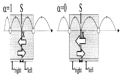
FIG. 1.: Particle flux for Brownian walkers with a step length depending on arrival position ($\alpha=1$) or departure position ($\alpha=0$).

As a result, in the situation of maximum drift where $\alpha=1$, this flux will vanish (see left part of Fig. 1), meaning that the uniform particle distribution corresponds to an equilibrium. According to Boltzmann, this should correspond to an isothermal situation, the diffusion coefficient gradient arising only from a pure hydrodynamic effect, the spatial dependence of the drag coefficient $\gamma$. For all the other values of $\alpha$, the flux will be negative, leading to a concentration gradient of the particles in the direction opposite to that of the diffusion coefficient gradient. The maximum flux (and zero drift) is obtained for $\alpha=0$, as shown on the right part of figure 1. Equation (7) may be generalized to the case where the particle distribution is position dependent:

$$J=-(1-\alpha)\rho(x){{dD}\over{dx}}-D{{d\rho}\over{dx}},$$ (8)

which leads to the well known generalization of Fick’s law for a space dependent diffusion coefficient[5].

To confirm these results, we performed simulations of Brownian walkers following algorithm (3). We found that only the $\alpha=1$ case leads to a uniform distribution of particles with no net flux through any given surface while, at the same time, the average individual positions exhibit a drift in the direction of the diffusion coefficient gradient according to Eq(4). This situation of “drift without flux” may be compared to the equilibrium situation of Brownian particles subjected to an external force, such as their weight: If one follows the motion of individual particles, an average downwards drift is observed; however, there is no net flux because of the vertical concentration gradient. In our isothermal case, the drift of individual particles from lower to larger D(x) region does not lead to a net flux because particles in the larger D(x) region diffuse further than particles in the lower D(x) region. This physical situation imposes the choice of $\alpha=1$ in algorithm (3), so that a particle coming from a low $D(x)$ region makes a right step just equal to the left step of that particle coming from a high $D(x)$ region and arriving at the same point (see left part of Fig. 1).

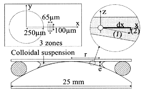
FIG. 2.: Experimental set-up. Rectangular inset is an enlarged top view showing the center of the cell with the circular excluded volume and the observation frame. Round inset explains the two contributions to the change in diffusion coefficient when a particle moves a distance dx.

We have set up an experiment to check this drift without flux prediction where particles, observed under a microscope, undergo Brownian motion in a confined geometry. When the confinement, $e$, is of the order of the particle size, $a$, the diffusion coefficient strongly depends on the value of $e/a$. As the confinement was position dependent, we observed Brownian walkers in an isothermal situation but with a spatially dependent $D(x)$ due to a purely hydrodynamic effect.

Polystyrene spheres, of radius $a=1\mu$m, were suspended in a mixture of $H_{2}O+D_{2}O$ so as to cancel any sedimentation effects. Addition of a surfactant ($2.2g/l$ of SDS) helped minimize particle aggregation or adhesion to the walls. A drop of this mixture was placed between a flat disk and a planar convex lens, Fig. (2), of curvature radius $R=15.5$mm separated by an elastic O-ring. The flat and convex surfaces were then brought into contact at the center of the cell by gently squeezing the elastic joint, the remaining air providing the necessary sample compressibility. The spacing, $e$, between the flat and curved wall depends on the distance $r$ from the center of the cell as $e=r^{2}/2R$. The contact between the two walls as well as the dependence of $e$ on $r$ were carefully measured by monitoring the Newton rings observed under the microscope. We used as a light source a new super-radiant diode[6] whose coherence length is less than $100\mu$m. This was important as this coherence length was long enough to observe the desired Newton rings, but short enough to avoid any other interference patterns due to all the cell interfaces, which were visible with an ordinary diode laser and which completely masked the relevant signal. The horizontal Brownian motion of the polystyrene balls was observed through a microscope equipped with a long range objective of magnification $50X$, followed by a CCD camera coupled to the microscope via an eyepiece of magnification $8X$. The video signal was processed in real time by a computer, which recorded, every $3$s the horizontal position, size and shape of all objects in a rectangular frame $65\mu{\rm m}X100\mu$m. This time interval was long enough to allow the image analysis of all particles present in the frame and small enough so that the particle’s average displacement was only a fraction of their diameter.

As the particles’ confinement, $e$, was related to their distance, $r$, from the center of the cell, we were able to explore different confinement regions by moving the observation frame in the horizontal plane. The explored $e$ varied from $2.5\mu$m to $11\mu$m. The vertical Brownian motion of the particles over this small vertical range could not be monitored. However, we took that motion into account when interpreting the data by averaging the particle’s vertical position over the confinement range. The volume fraction of polystyrene balls, of the order of $1\%$, was chosen so as to allow the monitoring of a fairly large number of particles at the same time (around $30$ for $e=3\mu$m) to improve the statistics in the data analysis. Following the particles’ positions from one frame to another, the program analyzed a great number of trajectories (more than $10^{5}$ for each run). When two particles got closer than twice their diameter, the program treated them as “dimers”, their trajectories as “monomers” were ended at that time and were no longer used to determine the diffusion coefficient or the drift. In that way, the role of particle interactions, which have a range smaller than a couple of particle diameters, could be safely ignored.

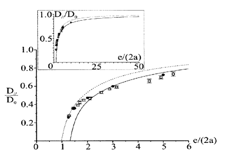
FIG. 3.: $D_{\parallel}/D_{0}$ with respect to relative confinement e/2a . Open squares are the experimental data, black dots were calculated by the collocation method, and dotted and solid lines follow analytical approximate solutions.

The confinement dependence of the diffusion coefficient was determined as follows. A given observation frame was divided into 3 zones (see inset, Fig. (2)), each corresponding to an approximately constant $e$. For each zone we averaged the particle’s displacement squared, either in the x, or in the y directions, as a function of time, and checked that indeed they followed the usual diffusion law,

$$\langle x^{2}\rangle=\langle y^{2}\rangle=2D_{\parallel}(e)t.$$ (9)

By moving the frame to different locations, we were able to explore a range extending from $e/2a=1.2$ to $11$. The bulk diffusion constant, $D_{0}$, was determined using the well-known relation $D_{0}=kT/6\pi\eta a$, where $\eta=0.99X10^{-3}$SI is the viscosity of the water- heavy water mixture, yielding $D_{0}=1.92X10^{-13}$m²/s. The experimental values for $D_{\parallel}/D_{0}$ are shown in Fig. (3) (white squares) and fit remarkably well the available theoretical predictions (black dots) using the collocation method[7] averaged over all the possible vertical positions $z$ of the particle for a given $e$, i.e. with $a\leq z\leq(e-a)$. For comparison, we also plotted (solid line) the analytical solution obtained using the Faxen expression[8] for the position dependent drag of a particle moving parallel to a single wall, then adding the effect of each of the two walls, and averaging over the vertical position $z$. This solution clearly overestimates the reduction of the diffusion coefficient of a particle trapped between two parallel walls, particularly as the relative confinement, $\epsilon=e/2a$ reaches its lower limit 1. We also plotted (dashed lines) in Fig. (3) the analytical expression for the drag of a particle trapped just in the middle of two parallel planes.[8] The impossibility of averaging over $z$ an expression only known for $z=e/2$ explains the observed discrepancy which goes to zero as the relative confinement approaches its limit, $1$, where the z-average becomes irrelevant.

To demonstrate the existence of an individual drift of the particles, we fixed the center of the observation frame at a position $y=0$ and $x=300\mu$m, corresponding to an average $e/2a=1.5$ so that all particles present in the frame were outside the excluded volume (i.e. $e\geq 2a$), and had a diffusion coefficient with the largest $x$ dependence, but no y dependence (to first order). For the determination of $\langle x(t)-x(0)\rangle$ and $\langle y(t)-y(0)\rangle$, each trajectory was divided into independent paths lasting a time $t$, each contributing to the evaluation of the average drift during time $t$. The results are shown in Fig. (4), and reveal a drift in the Brownian walker position along the $x$ direction, and none in the $y$ direction along which the diffusion coefficient may be considered as constant. The statistics of the results clearly deteriorates as time increases: After recording trajectories for typically a dozen hours, more than a hundred thousand independent segments contributed to the determination of the drift at short times, whereas only up to a few thousand independent segments were left for $t=200$s. This is due to the fairly high particle concentration which lowers the lifetime of a “monomer” (time during which a particle doesn’t approach another one to within 2 particle diameters), but which was chosen as a compromise to have good statistics at short times while allowing us to follow each particle during a reasonable time, fixed at $200$s. It should be pointed out that in order to avoid any bias in the statistics, for a trajectory segment to be valid and included in the statistics, the position of a walker at instant $t=0$ had to be inside a region $15\mu$m away from the edges of the observation frame. This condition ensured that after diffusing for $200$s, the walker had less than $0.5\%$ chance to have covered $15\mu$m, and was thus still present in the observation frame. Failure to impose this condition resulted in the observation of a spurious drift, in the opposite direction, due to an artificial selection of walkers because of the experimental boundary conditions (limits of the observation frame).

To compare our experimental results with the theoretical predictions, Eq. (4), we evaluated the diffusion gradient encountered by the walkers present in the observation frame. It is important to realize that as a walker moves a distance $dx$ (see round inset in Fig. 2), its diffusion coefficient $D_{\parallel}$ varies first because the confinement varies (path (1) parallel to the bottom wall, i.e. at constant $z$), and second because at constant confinement, the particle’s height $z$ changes (path (2)). Adding both contributions and averaging over the vertical position z of the walker yields:

$$\big{\langle}{{dD_{\parallel}(e,z)}\over{dx}}\big{\rangle}_{z}={x\over R}\big{\langle}{{\partial D_{\parallel}(e,z)}\over{\partial e}}\big{\rangle}_{z}+{{x}\over{2R}}\big{\langle}{{\partial D_{\parallel}(e,z)}\over{\partial z}}\big{\rangle}_{z}.$$ (10)

Using our experimental data and results of the collocation method, we found $\langle{{dD_{\parallel}(e,z)}/{dx}}\rangle_{z}\approx 2.2X10^{-9}$m/s. This value of the slope is used to plot the straight dotted line on Fig. 4. The experimental data are thus in good agreement with the predicted drift corresponding to the expected $\alpha=1$ value.

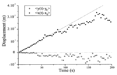
FIG. 4.: Average position of the walkers as a function of time, along (black dots) and perpendicular (open squares) to the diffusion gradient.

Finally, to claim drift without flux, it is not sufficient only to demonstrate the drift: we must also demonstrate the absence of flux. If a flux was due to the observed drift $dD/dx$, we would expect a radially outwards flux of $\rho dD/dx$ particles, which would empty our observation screen in less than a day. Furthermore, if this flux were to be balanced by a concentration gradient, one can show that a concentration change by $30\%$ over a distance of $60\mu$m would be necessary. Experimentally, we observed no flux and no concentration gradient over a period of a week or more, which is consistent with the Boltzmann requirement of a uniform concentration in the absence of a temperature gradient.

REFERENCES

- [1] J. Happel and H. Brenner, Low Reynolds number Hydrodynamics, Kluwer Academic Publishers (fifth printing 1991).
- [2] L.P. Faucheux and A.J. Libchaber, Phys. Rev. E49, 5158 (1994).
- [3] M.D. Carbajal-Timoco, G. Cruz de Léon, J.L. Arauz-Lara, Phys. Rev. E56, 6962 (1997).
- [4] H. Risken, The Fokker-Planck Equation, Springer-Verlag (1989).
- [5] M.J.Schnitzer, Phys. Rev. E48, 2553 (1993).
- [6] Kindly supplied by EPF (Lausanne) and MITEL Semiconductors (Stockholm).
- [7] P. Ganatos, S. Weinbaum and R. Pfeffer, J. Fluid Mech., 99, 755 (1980).
- [8] H. Faxen, Arkiv. Mat. Astron. Fys., 17, No 27 (1923).