Effective charges and statistical signatures in the noise of normal metal–superconductor junctions at arbitrary bias

Abstract

Shot noise is studied in a single normal metal-superconductor (N-S) junction at finite frequency, and for branched N-S junctions at zero frequency. The noise spectral density displays a singularity at the Josephson frequency ($\omega=2eV/\hbar$) when the applied bias is smaller than gap of the superconductor. Yet, in the limit $eV\gg\Delta$, quasiparticle contributions yield a singularity at $\omega=eV/\hbar$ analogous to that of a normal metal. The crossover between these two regimes shows new structures in the noise characteristic, pointing out the failure of the effective charge model. As an alternative to a finite frequency measurement, if a sinusoidal external field is superposed to the constant bias (non stationary Aharonov–Bohm effect), the second derivative of the zero frequency noise with respect to the voltage exhibits peaks when the frequency of the perturbation is commensurate with the Josephson frequency. Finally, the statistical aspects of noise are studied with an analog of the Hanbury-Brown and Twiss experiment for fermions: a superconductor connected to two normal leads. Noise correlations are found to be either negative (fermionic) or positive (bosonic), due to the presence of evanescent Cooper pairs in the normal side of the junction, in the latter case.

I Introduction

Recent developments in condensed matter physics emphasize the importance of shot noise in mesoscopic conductors. Noise contains more information than the conductance: in the Poisson regime for instance, zero-frequency noise is proportional to the current and to the effective charge. A convincing application is the direct measurement of the fractional charge in a quantum Hall liquid [1]. Another important issue of noise concerns the statistics of the (quasi-) particles. It is now established that Hanbury-Brown and Twiss [2] type correlation experiments yield a different sign for bosons and for fermions [3, 4, 5, 6].

This paper focuses on both issues in normal metal-superconductor (NS) junctions. Existing results on junctions between two normal metals (NN) are summarized below. Finite frequency shot noise has a singularity at $\hbar\omega=eV$ (where $V$ is the applied bias) [7], which was detected experimentally [8]. Another phenomenon, analogous to a finite frequency measurement, called the “Non-Stationary Aharonov–Bohm effect” [9] uses a local alternating field superposed to the bias voltage. Steps in the noise derivative with respect to the DC bias were predicted [9] and measured [10]. The height of these steps is non-monotonic with the amplitude of the harmonic perturbation.

The statistical signatures of noise correlations can be illustrated in a three terminal device where current fluctuations in the two receiving leads are expected to be fully anti-correlated [3, 4], a direct consequence of the Pauli principle. Experiments were performed in the integer quantum Hall regime [5] and in a two dimensional electron gas [6], with a splitter used to partition an incident beam of electrons into reflected and transmitted beams. The measurement of the correlations between the reflected and the transmitted beams reported a negative value, confirming the theoretical predictions.

In contrast to normal junctions, transport in NS junctions involves Andreev reflection [11]: an incoming electron is reflected as a hole at the boundary. The remaining charge $2e$ is absorbed by the superconductor via a Cooper pair. In a previous paper[12], finite frequency noise was computed in the Andreev regime only ($eV\ll\Delta$). The noise characteristics then present a singularity at the frequency $\omega=2eV/\hbar$, a signature of an effective charge $2e$ corresponding to that of a Cooper pair. This issue is not surprising, because in the Andreev regime, some physical quantities can, in principle, be extracted from the normal metal results by replacing $e$ by $2e$. In particular, at zero-frequency the doubling of shot noise and the crossover from thermal noise to excess noise have been predicted [13, 14, 15] and recently measured [16, 17]. However, for thermal noise (at $k_{B}T\ll\Delta$), this naive substitution would imply a violation of the fluctuation dissipation theorem.

Failures of this effective charge model also occur when the bias is comparable to the gap or when it is increased beyond it. Indeed, when $eV>\Delta$, the effective charge transfer picture breaks down, as quasi-particles above the gap bear a single electron charge. It will be shown that at such voltages, the cusps/singularities which appear in the finite frequency noise neither correspond to a charge $e$ nor to a charge $2e$. Thus, a careful analysis and an explicit calculation are especially needed to describe the crossover from sub-gap to above gap regime. Moreover, with the advent of superconducting samples with a “small” gap, this also allows to consider the limit of large biases ($eV\gg\Delta$), where single quasiparticle transmission overrides Andreev reflection. In this situation, one recovers the results obtained for the NN junctions, with a charge transfer $e$.

At the same time, an NS junction which contains a splitter on the normal side constitutes a Hanbury-Brown and Twiss type experiment where statistical effects can be detected [18]. In the Andreev regime, the noise correlations could possibly be positive (bosonic) due to the presence of Cooper pairs on the normal side (proximity effect), whereas a quasi-particle dominated regime should favor negative (fermionic) correlations. The purpose is here to investigate the effective charges and statistical tendencies which show up in the noise characteristics of an NS junction in an united fashion. Results for the sub-gap (Andreev) regime will be recalled, and confronted to novel results for above gap transport.

The paper is organized as follows. Noise correlations in a multi-terminal device coupled with a superconductor are computed at finite frequencies (section II). In section III a single N-S junction is studied for several cases: a) in the Andreev regime (section III B), the noise spectral density presents a singularity at the Josephson frequency; b) when the applied bias is increased beyond the gap (section III C), additional singularities appear; c) if a sinusoidal external field is added (non-stationary Aharonov-Bohm effect, section III D), the second derivative of noise with respect to the bias presents peaks when the frequency of the perturbation is commensurate with the Josephson frequency. The last section (IV) deals with the fermionic Hanbury-Brown and Twiss experimental proposal with a superconductor, showing that noise correlations may be either negative or positive.

II Current, noise and noise correlations

A Assumptions

The superconductor is connected to an arbitrary number of normal leads (multi-terminal device), and the device is supposed to be small enough that all scattering processes are elastic. Note that the case of two superconductors is not addressed here (see Ref. [19]). Calculations are restricted to the one-channel case, but a generalization to a multi-channel system is straightforward. Thus, transport is dominated by the scattering properties of the N-S junction [20, 21, 22, 23]. The two scattering processes at play are then Andreev reflection and normal reflection of electrons and holes. The superconductor is maintained at a constant chemical potential $\mu_{S}$, and each normal terminal is fixed at the same potential $\mu_{N}$. For convenience, all energies are measured with respect to $\mu_{S}$, so that the applied bias reads $\mu_{N}-\mu_{S}=eV$. This bias is chosen to be positive throughout the paper.

Shot noise in a given lead, or alternatively noise correlations between two (normal) terminals are defined as the Fourier transform of the current-current correlation function:

$$S_{ij}(\omega) = \lim_{T\rightarrow+\infty}\frac{1}{T}\int_{-T/2}^{T/2}dt\int_{-\infty}^{+\infty}dt^{\prime}e^{i\omega t^{\prime}}$$ (2)

$$\hskip 42.67912pt\Bigl{(}\langle I_{i}(t)I_{j}(t+t^{\prime})\rangle-\langle I_{i}\rangle\langle I_{j}\rangle\Bigr{)}~{}.$$

When $i=j$, $S_{ii}(\omega)$ corresponds to the noise in the terminal $i$, whereas if $i$ and $j$ are different, $S_{ij}(0)$ represents the zero frequency noise correlations between lead $i$ and lead $j$. $\langle~{}\rangle$ designates the thermodynamical average in the grand-canonical ensemble.

B Bogolubov-de Gennes equations

The Bogolubov-de Gennes [24] (BdG) approach to inhomogeneous superconductivity is the adapted formalism to treat electrons and holes on the same footing. Performing the Bogolubov transformation (which must diagonalize the effective BdG Hamiltonian), and going to an energy representation, the annihilation operator of a particle with spin $\sigma$ ($\sigma=\pm 1$) at the position $x$ in the terminal $i$ $\psi_{i,\sigma}(x)$ can be written as:

$$\psi_{i,\sigma}(x) = \frac{1}{\sqrt{2\pi}}\sum_{j}\sum_{\beta}\int_{0}^{+\infty}dE\left(\frac{u_{i\,j\,\beta}(x)}{\sqrt{\hbar v^{j}_{e}(E)}}c_{j\,\beta\,\sigma}(E)\right.$$ (3)

$$\hskip 42.67912pt\left.-\sigma\frac{v_{i\,j\,\beta}^{*}(x)}{\sqrt{\hbar v^{j}_{h}(E)}}c^{+}_{j\,\beta\,-\sigma}(E)\right)~{}.$$ (4)

State $u_{i\,j\,\beta}$ ($v_{i\,j\,\beta}$) corresponds to the wave function of a electron (a hole) scattered in terminal $i$, due to a quasi-particle of type $\beta$ (electron or hole, $\beta=e,h$) which was incoming from lead $j$. Operators $c(E)$ and $c^{+}(E)$ satisfy standard anticommutation relations. $v^{j}_{e}(E)=\hbar k_{e}^{j}(E)$ is the velocity in the lead $j$. The Bogolubov-de Gennes equations may be written as:

$$\left\{\begin{array}[]{llll}Eu_{i\,j\,\beta}(x)&=&&\!\!\!\left(-\displaystyle\frac{\hbar^{2}}{2m}\frac{\partial^{2}}{\partial x^{2}}-\mu_{S}+V(x)\right)u_{i\,j\,\beta}(x)\\ \\ &&&\hskip 56.9055pt+\Delta(x)v_{i\,j\,\beta}(x)~{},\\ \\ Ev_{ij\beta}(x)&=&-&\!\!\!\left(-\displaystyle\frac{\hbar^{2}}{2m}\frac{\partial^{2}}{\partial x^{2}}-\mu_{S}+V(x)\right)v_{i\,j\,\beta}(x)\\ \\ &&&\hskip 56.9055pt+\Delta^{*}(x)u_{i\,j\,\beta}(x)~{},\end{array}\right.$$ (5)

and describe the evolution of particle states $u_{i\,j\,\beta}$ and $v_{i\,j\,\beta}$. The pair potential $\Delta(x)$ should be calculated self-consistently, but for simplicity corresponds here to the superconducting gap in the bulk superconductor ($x>0$), and gives zero in the normal terminals ($x<0$).

C States in a normal terminal

In order to calculate noise with Eq. (2), the states which appear in the Bogolubov transformation (4) are specified using the scattering ($S$) matrix describing the junction. In a normal, ideal lead $\Delta(x)=0$ and $V(x)=0$, the Bogolubov-de Gennes equations (5) reduces to a Schrödinger equation for electrons, and to its time reversed analog for holes. Solutions of the form $e^{ik^{N}_{e}x}$ for electrons, and $e^{ik^{N}_{h}x}$ for holes are chosen, where $k^{N}_{e}=\sqrt{2m\left(\mu_{S}+E\right)}/\hbar$ and $k^{N}_{h}=\sqrt{2m\left(\mu_{S}-E\right)}/\hbar$ are the wave vectors of electrons and holes. Electrons and holes in lead $i$ which originate from a particle of type $\beta$ ($\beta=e,h$) in terminal $j$ and scattered into $i$ are described by:

$$u_{i\,j\,\beta}(x) = \delta_{i,j}\delta_{e,\beta}e^{ik^{N}_{e}x}+s_{ije\beta}\sqrt{\frac{k^{j}_{\beta}}{k^{N}_{e}}}e^{-ik^{N}_{e}x}~{},$$ (6)

$$v_{i\,j\,\beta}(x) = \delta_{i,j}\delta_{h,\beta}e^{-ik^{N}_{h}x}+s_{ijh\beta}\sqrt{\frac{k^{j}_{\beta}}{k^{N}_{h}}}e^{ik^{N}_{h}x}~{}.$$ (7)

Note the opposite sign for momenta of electrons and holes. $x_{i}$, the position in terminal $i$ is specified as $x$ in Eqs. (6) and (7) for simplicity of notation. $s_{ij\alpha\beta}$ is the scattering matrix element expressing the amplitude of an outgoing particle $\alpha$ in lead $i$ due to an incident particle of type $\beta$ in lead $j$.

D Current operator and average current

The current operator in lead $i$ is defined by:

$$I_{i}(x) = e\frac{\hbar}{2mi}\sum_{\sigma}\left(\psi^{+}_{i,\sigma}(x)\frac{\partial\psi_{i,\sigma}(x)}{\partial x}\right.$$ (9)

$$\hskip 56.9055pt\left.-\frac{\partial\psi^{+}_{i,\sigma}(x)}{\partial x}\psi_{i,\sigma}(x)\right)~{}.$$

Substituting $\psi$ by Eq. (4), the current operator becomes:

$$I_{i}(x) = \frac{e\hbar}{2miv_{F}}\frac{1}{2\pi\hbar}\int_{0}^{+\infty}dE_{1}\int_{0}^{+\infty}dE_{2}\sum_{m,n}\sum_{\sigma}$$ (14)

$$\hskip 25.6073pt\Bigl{[}\Bigl{(}u_{im}^{*}\partial_{x}u_{in}-\partial_{x}u_{im}^{*}u_{in}\Bigr{)}c^{+}_{m\,\sigma}c_{n\,\sigma}$$

$$\hskip 25.6073pt-\Bigl{(}u_{im}^{*}\partial_{x}v_{in}^{*}-\partial_{x}u_{im}^{*}v_{in}^{*}\Bigr{)}\sigma\,c^{+}_{m\,\sigma}c^{+}_{n\,-\sigma}$$

$$\hskip 25.6073pt-\Bigl{(}v_{im}\partial_{x}u_{in}-\partial_{x}v_{im}u_{in}\Bigr{)}\sigma\,c_{m\,-\sigma}c_{n\,\sigma}$$

$$\hskip 25.6073pt+\Bigl{(}v_{im}\partial_{x}v_{in}^{*}-\partial_{x}v_{im}v_{in}^{*}\Bigr{)}c_{m\,-\sigma}c^{+}_{n\,-\sigma}\Bigr{]}~{},$$

where the sums over $j$ and $\beta$ have been replaced by a single sum over index $m$. Expressions with index $m$ ($n$) have an energy dependence $E_{1}$ ($E_{2}$). Solving the Bogolubov-de Gennes equations in the superconductor leads to find the waves vectors $k^{S}_{e,h}=\sqrt{2m}\left(\mu_{S}\pm\left(E^{2}-\Delta^{2}\right)^{1/2}\right)^{1/2}/\hbar$ for electron-like (+) and hole-like (-) quasi-particles. The chemical potential of the superconductor $\mu_{S}$ is large compared to all the energy scales involved in the system. Thus, the assumption $k^{N}_{e}=k^{N}_{h}=k^{S}_{e}=k^{S}_{h}=k_{F}$ is made, which explains the presence of the Fermi velocity $v_{F}$ in Eq. (14).

The calculation of the average current involves the average of creation and annihilation operators products such as $\langle c^{+}_{m\,\sigma}(E_{1})c_{n\,\sigma}(E_{2})\rangle=f_{m}(E_{1})\delta_{mn}\delta(E_{1}-E_{2})$. $f_{m}(E)=f_{FD}(E\mp eV)$ for electrons and holes on the normal side, with $f_{FD}(E)$ the Fermi-Dirac distribution. $f_{m}(E)=f_{FD}(E)$ in the superconductor. The average current is then:

$$\langle I_{i}(x)\rangle = \frac{e}{2\pi miv_{F}}\int_{0}^{+\infty}dE\sum_{m}$$ (17)

$$\hskip 14.22636pt\Biggl{[}\Bigl{(}u_{im}^{*}\partial_{x}u_{im}-\partial_{x}u_{im}^{*}u_{im}\Bigr{)}f_{m}$$

$$\hskip 14.22636pt+\Bigl{(}v_{im}\partial_{x}v_{im}^{*}-\partial_{x}v_{im}v_{im}^{*}\Bigr{)}\left(1-f_{m}\right)\Biggr{]}~{}.$$

E Noise and noise correlations

Since a single current operator is composed of products of two creators or annihilators, $\langle I_{i}(x,t)I_{j}(x,t+t^{\prime})\rangle$ is a sum of average values of four creation or annihilation operators. These average values are expressed as a function of the Fermi-Dirac distributions using Wick’s theorem. The calculation of noise is now performed using Eq. (2). It is convenient to define the following matrix elements:

$$A_{imjn}(E,E^{\prime},t) = u_{jn}(E^{\prime},t)\partial_{x}u^{*}_{im}(E,t)$$ (19)

$$-u^{*}_{im}(E,t)\partial_{x}u_{jn}(E^{\prime},t)~{},$$

$$B_{imjn}(E,E^{\prime},t) = v^{*}_{jn}(E^{\prime},t)\partial_{x}v_{im}(E,t)$$ (21)

$$-v_{im}(E,t)\partial_{x}v^{*}_{jn}(E^{\prime},t)~{},$$

$$C_{imjn}(E,E^{\prime},t) = u_{jn}(E^{\prime},t)\partial_{x}v_{im}(E,t)$$ (23)

$$-v_{im}(E,t)\partial_{x}u_{jn}(E^{\prime},t)~{}.$$

Calculating all the average values and the difference $\langle I_{i}(t)I_{j}(t+t^{\prime})\rangle-\langle I_{i}\rangle\langle I_{j}\rangle$, one obtains the noise or the noise correlations:

$$S_{ij}(\omega) = \frac{e^{2}\hbar^{2}}{2m^{2}v_{F}^{2}}\frac{1}{\left(2\pi\hbar\right)^{2}}\lim_{T\rightarrow+\infty}\frac{1}{T}\int_{-T/2}^{+T/2}\!\!\!dt\int_{-\infty}^{+\infty}\!\!\!dt^{\prime}e^{i\omega t^{\prime}}$$ (36)

$$\hskip 14.22636pt\times\int_{0}^{+\infty}\!\!\!dE\int_{0}^{+\infty}\!\!\!dE^{\prime}\sum_{m,n}\Biggl{\{}$$

$$\hskip 14.22636ptf_{m}(E)(1-f_{n}(E^{\prime}))e^{i(E^{\prime}-E)t^{\prime}/\hbar}$$

$$\hskip 14.22636pt\times\Bigl{[}A_{imjn}(E,E^{\prime},t)A^{*}_{imjn}(E,E^{\prime},t+t^{\prime})$$

$$\hskip 14.22636pt+B^{*}_{imjn}(E,E^{\prime},t)B_{imjn}(E,E^{\prime},t+t^{\prime})$$

$$\hskip 14.22636pt+A_{imjn}(E,E^{\prime},t)B_{imjn}(E,E^{\prime},t+t^{\prime})$$

$$\hskip 14.22636pt+B^{*}_{imjn}(E,E^{\prime},t)A^{*}_{imjn}(E,E^{\prime},t+t^{\prime})\Bigr{]}$$

$$\hskip 14.22636pt+f_{m}(E)f_{n}(E^{\prime})e^{-i(E+E^{\prime})t^{\prime}/\hbar}\,C^{*}_{imjn}(E,E^{\prime})$$

$$\hskip 28.45274pt\times\Bigl{(}C_{\j nim}(E^{\prime},E,t+t^{\prime})$$

$$\hskip 56.9055pt+C_{imjn}(E,E^{\prime},t+t^{\prime})\Bigr{)}$$

$$\hskip 14.22636pt+(1-f_{m}(E))(1-f_{n}(E^{\prime}))e^{i(E+E^{\prime})t^{\prime}/\hbar}$$

$$\hskip 14.22636pt\times\Bigl{(}C_{\j nim}(E^{\prime},E,t)+C_{imjn}(E,E^{\prime},t)\Bigr{)}$$

$$\hskip 28.45274pt\times C^{*}_{imjn}(E,E^{\prime},t+t^{\prime})\Biggr{\}}~{}.$$

So far as the process is stationary (for example if no time dependent external field is applied), matrix elements $A_{imjn}$, $B_{imjn}$ et $C_{imjn}$ are time independent. As a consequence, the integration over $t$ simplifies, and the integration over $t^{\prime}$ gives $\delta$ functions with energy. As a result, terms proportional to $(1-f_{m})(1-f_{n})$ cancels because one is dealing with quasi-particles with a positive energy. This yields:

$$S_{ij}(\omega) = \frac{e^{2}\hbar^{2}}{2m^{2}v_{F}^{2}}\frac{1}{2\pi\hbar}\int_{0}^{+\infty}\!\!\!dE\sum_{m,n}\Biggl{\{}$$ (47)

$$\hskip 5.69054pt\Theta(E+\hbar\omega)f_{m}(E+\hbar\omega)(1-f_{n}(E))$$

$$\hskip 8.53581pt\times\bigl{|}A_{imjn}(E+\hbar\omega,E)+B^{*}_{imjn}(E+\hbar\omega,E)\bigr{|}^{2}$$

$$\hskip 5.69054pt+\Theta(\hbar\omega-E)f_{m}(\hbar\omega-E)f_{n}(E)$$

$$\hskip 28.45274pt\times C^{*}_{imjn}(\hbar\omega-E,E,t)$$

$$\hskip 28.45274pt\times\Bigl{(}C_{\j nim}(E,\hbar\omega-E)$$

$$\hskip 56.9055pt+C_{imjn}(\hbar\omega-E,E)\Bigr{)}$$

$$\hskip 5.69054pt+\Theta(-E-\hbar\omega)(1-\!f_{m}(-E-\hbar\omega))(1-\!f_{n}(E))$$

$$\hskip 14.22636pt\times C^{*}_{imjn}(-E-\hbar\omega,E)$$

$$\hskip 14.22636pt\times\Bigl{(}C_{\j nim}(E,-E-\hbar\omega)$$

$$\hskip 56.9055pt+C_{imjn}(-E-\hbar\omega,E)\Bigr{)}\Biggr{\}}~{},$$

after integration over $E^{\prime}$. This expression corresponds to the noise if indices $i$ and $j$ are the same:

$$S_{ii}(\omega) = \frac{e^{2}\hbar^{2}}{2m^{2}v_{F}^{2}}\frac{1}{2\pi\hbar}\int_{0}^{+\infty}\!\!\!dE\sum_{m,n}\Biggl{\{}$$ (57)

$$\hskip 5.69054pt\Theta(E+\hbar\omega)f_{m}(E+\hbar\omega)(1-f_{n}(E))$$

$$\hskip 14.22636pt\times\bigl{|}A_{imin}(E+\hbar\omega,E)+B^{*}_{imin}(E+\hbar\omega,E)\bigr{|}^{2}$$

$$\hskip 5.69054pt+\Theta(\hbar\omega-E)f_{m}(\hbar\omega-E)f_{n}(E)$$

$$\hskip 14.22636pt\times C^{*}_{imin}(\hbar\omega-E,E,t)$$

$$\hskip 14.22636pt\times\Bigl{(}C_{inim}(E,\hbar\omega-E)+C_{imin}(\hbar\omega-E,E)\Bigr{)}$$

$$\hskip 5.69054pt+\Theta(-E-\hbar\omega)(1-f_{m}(-E-\hbar\omega))(1-f_{n}(E))$$

$$\hskip 14.22636pt\times C^{*}_{imin}(-E-\hbar\omega,E)$$

$$\hskip 14.22636pt\times\Bigl{(}C_{inim}(E,-E-\hbar\omega)$$

$$\hskip 56.9055pt+C_{imin}(-E-\hbar\omega,E)\Bigr{)}\Biggr{\}}~{}.$$

The zero-frequency limit for noise correlations between terminals $i$ and $j$ yields [15, 19, 25, 26]:

$$S_{ij}(0) = \frac{e^{2}\hbar^{2}}{2m^{2}v_{F}^{2}}\frac{1}{2\pi\hbar}\int_{0}^{+\infty}\!\!\!dE\sum_{m,n}f_{m}(E)(1-f_{n}(E))$$ (59)

$$\hskip 28.45274pt\times\bigl{|}A_{imjn}(E,E)+B^{*}_{imjn}(E,E)\bigr{|}^{2}~{}.$$

III Single N-S junction

A General expression for noise

A single N-S junction with arbitrary transparency (with a tunneling barrier at the interface) is considered first for a small applied bias (Andreev regime $eV\ll\Delta$) and then for biases larger than the gap. Analytical expressions are obtained in the first case, while numerical results will be presented in the latter regime. For simplicity, the temperature is chosen to be much smaller than the gap in both cases. In the the Andreev regime, the integrals over energy in Eq. (57) can be performed, resulting in three distinct contributions combining different products of Fermi-Dirac distributions. It is interesting to note that although the current operator of Eq. (14) itself cannot couple states which differ by two quasi-particles, its fluctuations give a contribution which is proportional to $f_{n}f_{m}$ in this finite frequency calculation. Rewriting down $A_{mn}$, $B_{mn}$ and $C_{mn}$ as a function of the $S$ matrix elements, three distinct expressions of the noise are found. If $\hbar\omega<eV$:

$$S(\omega) = \frac{2e^{2}}{h}\Biggl{\{}\int_{0}^{eV-\hbar\omega}dE$$ (69)

$$\hskip 5.69054pt\times\Bigl{[}|s_{NNee}(E+\hbar\omega)|^{2}\left(1-|s_{NNee}(E)|^{2}\right)$$

$$\hskip 17.07164pt+|s_{NNhe}(E+\hbar\omega)|^{2}\left(1-|s_{NNhe}(E)|^{2}\right)$$

$$\hskip 17.07164pt+s_{NNee}^{*}(E+\hbar\omega)\;s_{NNee}(E)$$

$$\hskip 25.60747pt\times\;s_{NNhe}(E+\hbar\omega)\;s_{NNhe}^{*}(E)$$

$$\hskip 17.07164pt+s_{NNee}(E+\hbar\omega)\;s_{NNee}^{*}(E)$$

$$\hskip 25.60747pt\times\;s_{NNhe}^{*}(E+\hbar\omega)\;s_{NNhe}(E)\Bigr{]}$$

$$\hskip 2.84526pt+\int_{0}^{\hbar\omega}dE\Bigl{[}|s_{NNee}(E)|^{2}|s_{NNhe}(\hbar\omega-E)|^{2}$$

$$\hskip 8.53581pt+s_{NNee}(\hbar\omega-E)\;s_{NNhe}(E)$$

$$\hskip 25.60747pt\times\;s_{NNee}^{*}(E)\;s_{NNhe}^{*}(\hbar\omega-E)\Bigr{]}\Biggr{\}}~{}.$$

If $eV<\hbar\omega<2eV$, one obtains:

$$S(\omega) = \frac{2e^{2}}{h}\int_{\hbar\omega-eV}^{eV}dE\Bigl{[}|s_{NNee}(E)|^{2}|s_{NNhe}(\hbar\omega-E)|^{2}$$ (72)

$$\hskip 48.36958pt+s_{NNee}(\hbar\omega-E)\;s_{NNhe}(E)$$

$$\hskip 54.06006pt\times s^{*}_{NNee}(E)\;s^{*}_{NNhe}(\hbar\omega-E)\Bigr{]}~{}.$$

If $\hbar\omega>2eV$ noise vanishes. Eq. (72) contains no spatial dependence as a consequence of the approximation $\mu_{S}\gg\hbar\omega,eV$ mentioned in Sec. (II C).

B Small biases: Andreev regime

When the applied bias is much smaller than the gap, the $S$ matrix elements can be taken to be constant. Using the unitarity of the $S$ matrix, both expressions (69) and (72) are unified in the same formula over the whole energy interval $0<\hbar\omega<2eV$:

$$\left\{\begin{array}[]{llll}S(\omega)&=&\displaystyle\frac{4e^{2}}{h}(2eV-\hbar\omega)R_{A}(1-R_{A})&\mbox{if $\hbar\omega<2eV$}~{},\\ \\ S(\omega)&=&0&\mbox{if $\hbar\omega>2eV$}~{},\end{array}\right.$$ (73)

where $R_{A}=|s_{NNhe}(0)|^{2}$ is the Andreev reflection probability. The noise spectral density decreases linearly with frequency, and vanishes beyond the Josephson frequency $2eV/\hbar$ (figure 1), thus displaying a singularity at this frequency.

This result has to be compared with both the Josephson effect [27] and with the analog result for a normal metal junction [7] (figure 1). In the former case, a DC bias applied to a junction between two superconductors generates an oscillatory current. The order parameter on each side oscillates as $\psi_{1,2}\sim\exp[-i2\mu_{S_{1,2}}t/\hbar]$ with $\mu_{S_{1}}$ and $\mu_{S_{2}}$ the chemical potentials of each superconductor (figure 2a). The resulting current involves the overlap of these two states $\psi_{1}\psi_{2}^{*}$, and therefore oscillates at the frequency $2|\mu_{S_{2}}-\mu_{S_{1}}|/\hbar$. The noise characteristic exhibits a peak at $2eV/\hbar$ which radiation line-width was computed in Ref. [28] (inset figure 1). In the former case (figure 2b), the wave functions have a time dependence as $\psi_{1,2}\sim\exp[-i\mu_{1,2}t/\hbar]$, so that although the resulting current is constant, finite frequency noise involves the overlap $\psi_{1}\psi_{2}^{*}$ leading to a singularity at the frequency $|\mu_{2}-\mu_{1}|/\hbar=eV/\hbar$.

In the N-S case (figure 2c), only Andreev reflection contributes to the current, involving the emission or the absorption of Cooper pairs (charge $2e$) on the superconducting side. An incoming electron in the normal side at energy $\mu_{S}+eV$ drags another electron at energy $\mu_{S}-eV$, forming a reflected hole of energy $\mu_{S}-eV$. The two combined electrons have a total energy $2\mu_{S}$ which corresponds to a Cooper pair, and are thus allowed to be transfered to the superconducting side. Now the above argument for an oscillatory time dependence can be repeated, since the incoming electron wave function oscillates as $\psi_{e}\sim\exp[-i(\mu_{S}+eV)t/\hbar]$, whereas the hole wave function oscillates as $\psi_{h}\sim\exp[-i(\mu_{S}-eV)t/\hbar]$. The noise combines these dependences in the product $\psi_{e}\psi_{h}^{*}$ which now oscillates at the Josephson frequency $2eV/\hbar$ corresponding to the singularity. In a junction containing a single superconductor, the singularity therefore appears in the noise rather than the current, and the detection of this frequency can be considered as an analog to the Josephson effect.

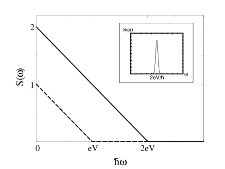
FIG. 1.: Noise as a function of frequency. Full line: N-S junction, with a singularity at $\hbar\omega=2eV$ (in units of $(4e^{2}/h)eVR_{A}(1-R_{A})$); dashed line: junction between two normal metals with a singularity at $\hbar\omega=eV$ (in units of $(4e^{2}/h)eVT(1-T)$). Inset: noise in the Josephson effect, with a peak at the frequency $\hbar\omega=2eV$.

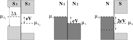
FIG. 2.: Three different kinds of junctions: a) two superconductors in contact (Josephson effect), with chemical potentials $\mu_{S_{1}}$ and $\mu_{S_{2}}$; b) two normal metals with chemical potentials $\mu_{1}$ and $\mu_{2}$; c) a normal metal ($\mu_{N}$) connected to a superconductor ($\mu_{S}$).

C Large biases

The applied bias is now larger than (or comparable to) the gap, so that the scattering matrix elements depends on the energy. A specific description is needed to characterize this dependence: the BTK model [29] is particularly suited for this purpose as it allows a description with a minimal number of parameters.

A local tunnel barrier $V_{B}(x)=V_{B}\delta(x)$ is introduced at the boundary. Since the complete knowledge of the $S$ matrix of the junction is necessary to compute the noise, the quasi-particle states in the superconductor are specified. This only makes sense if these states are not evanescent ($E>\Delta$). The Bogolubov-de Gennes equations for these states are solved on the superconducting side. Using the continuity of the wave functions at the interface, and specifying the discontinuity of their derivative, one obtains the $S$ matrix elements (Appendix A).

The energy integrals in Eqs. (69) and (72) are performed numerically. Plotting the noise as a function of frequency, additional cusps or singularities are found at $\omega=(eV-\Delta)/\hbar$, $\omega=(2\Delta)/\hbar$, $\omega=(eV+\Delta)/\hbar$, on top of the Josephson singularity at $\omega=2eV/\hbar$ (figure 3). All these frequencies can be illustrated on an energy diagram (figure 4). This numerical calculation can also be performed for small biases, yielding full agreement with the previous calculation (73). Another interesting limit arises when $eV\gg\Delta$. In this case, transport is dominated by single quasi-particle transfer with a charge $e$, whereas the contribution of Andreev reflection is small. Thus similar results to those of normal-normal metals junction are expected. This is obviously the case (figure 5), even though the above mentioned singularities can still be identified. One may object that if the applied bias is too large, the non-equilibrium processes dominate, and the previous assumptions are not correct anymore because of heating effects. This limit is then valid for superconductors with a small gap ($\Delta/k_{B}\sim 0.1K$) because the condition $eV\gg\Delta$ may be satisfied in a near-equilibrium situation.

In order to visualize the additional singularities, the argument invoking the oscillatory time dependence can be used once again. This time, because of the large value of the bias, several charge transfer processes occur: a) Andreev reflection is still there, and it implies the same singularity at the Josephson frequency $2eV/\hbar$. b) Electrons in the normal side are transmitted as electron-like quasi-particles in the superconductor. Wave functions oscillate as $\psi_{N,e}\sim\exp[-i(\mu_{S}+eV)t/\hbar]$ and $\psi_{S,e}\sim\exp[-i(\mu_{S}+\Delta)t/\hbar]$, and the overlap gives a singularity at $(eV-\Delta)/\hbar$. Note that the same transfer process occurs with holes and hole-like quasi-particles, giving the same singularity. c) Electrons in the normal side are transmitted as hole-like quasi-particles in the superconductor (Andreev transmission). Here, the time dependence of the wave functions is $\psi_{N,e}\sim\exp[-i(\mu_{S}+eV)t/\hbar]$ and $\psi_{S,h}\sim\exp[-i(\mu_{S}-\Delta)t/\hbar]$, implying a singularity at $(eV+\Delta)/\hbar$. The same transfer process exists with holes and electron-like quasi-particles. d) Andreev reflection also occurs on the superconducting side, when electron-like quasi-particles are reflected as hole-like quasi-particles, and vice versa. Wave functions oscillates as $\psi_{S,e}\sim\exp[-i(\mu_{S}+\Delta)t/\hbar]$ and $\psi_{S,h}\sim\exp[-i(\mu_{S}-\Delta)t/\hbar]$, giving a singularity at the frequency $2\Delta/\hbar$. These four singularities are summarized in Fig. 3.

FIG. 3.: Noise in a N-S junction as a function of frequency, with intermediate barrier transparency ($Z=1$), for several values of the applied bias : $eV=0.8\Delta$, $eV=1.3\Delta$, $eV=1.9\Delta$.

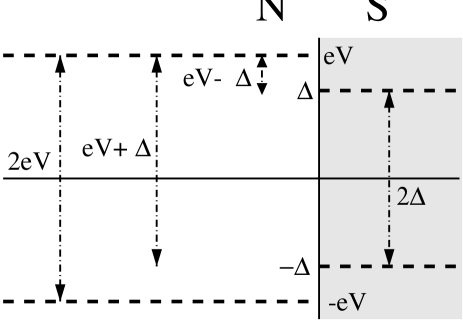
FIG. 4.: Energy diagram when the bias is larger than the gap. Relevant intervals associated with the cusps/singularities are shown.

FIG. 5.: Noise in a N-S junction as a function of frequency, with intermediate barrier transparency ($Z=1$), for a large value of the bias ($eV=20\Delta$).

D Non-stationary Aharonov-Bohm effect

Finite frequency measurements can represent a real challenge for noise, so it is interesting to imagine a scenario where an alternating field superposed to the DC bias allows to probe the finite frequency effect. The non-stationary Aharonov–Bohm effect has been introduced several years ago in a normal conductor connected to reservoirs [9]. In this proposal, a time dependent vector potential is applied in a confined region $[x_{1},x_{2}]$ of the conductor, which adds a phase to the electrons and holes. The phase is chosen to be a periodic function of time $\Phi(t)=\Phi_{a}\sin(\Omega t)$ with $\Phi_{a}\equiv 2\pi\int_{x_{1}}^{x_{2}}dxA_{x}/\phi_{0}$, and where $\phi_{0}=hc/e$ is the normal flux quantum. The most striking consequence is the presence of steps in the derivative of the shot noise with respect to the voltage $\partial S/\partial eV$ when the applied bias $eV$ is a multiple of the frequency of the perturbation $\hbar\Omega$. Moreover, the gaps between the steps are non-monotonic with the amplitude of the harmonic vector potential. This effect has been experimentally observed in normal diffusive samples [10].

Here, this result is extended to an N-S junction using the same framework (figure 6). The perturbation remains confined in the interval $[x_{1},x_{2}]$ near the boundary and is assumed to contain an adiabatic time modulation. The main difference with the previous case is due to the Andreev reflection. The wave function of an incoming electron accumulates a phase $\Phi(t)$ in the region where the potential is confined, but after a normal reflection the same phase is subtracted. On the contrary, if the electron is Andreev reflected, the outgoing hole accumulates a phase $\Phi$, totalizing a phase $2\Phi$ for the complete reflection process. So in the Andreev regime, the $S$ matrix of the junction can be written as follow:

$$S=\left(\begin{array}[]{cc}s_{ee}&s_{eh}\,e^{-2i\Phi(t)}\\ s_{he}\,e^{2i\Phi(t)}&s_{hh}\end{array}\right)~{},$$ (74)

where $s_{ee}$, $s_{eh}$, $s_{he}$ and $s_{hh}$ are the standard matrix elements describing the N-S boundary only (without the external time perturbation).

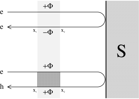
FIG. 6.: The NS boundary. The light shaded region determines where the electron/hole wave function may accumulate phase: schematic description of the two scattering processes, Andreev and normal reflection.

In contrast to the usual Aharonov-Bohm effect, no closed topology is imposed: the flux does not have to be enclosed in a loop, and the current is not periodic in the accumulated phase $2\Phi(t)$. Moreover, the effect of the perturbation on the average current is straightforward in the limit where the probability of Andreev reflection $R_{A}$ depends weakly on the energy: it brings a periodic modulation of the current $\Delta I=(4e^{2}/h)R_{A}[\hbar\Omega/e]\Phi_{a}\cos(\Omega t)$. The most striking consequence of the flux occurs when the current-current correlations are considered: the modulation leads to a non-monotonic effect as a function of phase, in contrast with the electromotive force action on the current.

However, because of this periodic perturbation, translational invariance in time is broken, and the process becomes non-stationary. So the noise depends in general on two frequencies and thus can be written as:

$$\widetilde{S}(\Omega_{1},\Omega_{2}) = \int\int dt_{1}dt_{2}e^{i\left(\Omega_{1}t_{1}+\Omega_{2}t_{2}\right)}$$ (76)

$$\hskip 42.67912pt\Bigl{(}\langle I(t_{1})I(t_{2})\rangle-\langle I\rangle^{2}\Bigr{)}~{}.$$

This double Fourier transform can be rewritten as:

$$\widetilde{S}(\Omega_{1},\Omega_{2})=\sum_{m=-\infty}^{+\infty}2\pi\delta(\Omega_{1}+\Omega_{2}-m\Omega)S^{(m)}(\Omega_{2})~{}.$$ (77)

The zero harmonic, which is proportional to $\delta(\Omega_{1}+\Omega_{2})$ is the most standard quantity to study. From Eq. (36), its zero-frequency expression is given by:

$$S^{(0)}(0) = \frac{e^{2}\hbar^{2}}{2m^{2}v_{F}^{2}}\frac{1}{\left(2\pi\hbar\right)^{2}}\int_{-\infty}^{+\infty}\!\!\!dt\int_{-\infty}^{+\infty}\!\!\!dt^{\prime}$$ (90)

$$\hskip 14.22636pt\times\int_{0}^{+\infty}\!\!\!dE\int_{0}^{+\infty}\!\!\!dE^{\prime}\sum_{m,n}\Biggl{\{}$$

$$\hskip 14.22636ptf_{m}(E)(1-f_{n}(E^{\prime}))e^{i(E^{\prime}-E)(t^{\prime}-t)/\hbar}$$

$$\hskip 14.22636pt\times\Bigl{[}A_{NmNn}(E,E^{\prime},t)A^{*}_{NmNn}(E,E^{\prime},t^{\prime})$$

$$\hskip 14.22636pt+B^{*}_{NmNn}(E,E^{\prime},t)B_{NmNn}(E,E^{\prime},t^{\prime})$$

$$\hskip 14.22636pt+A_{NmNn}(E,E^{\prime},t)B_{NmNn}(E,E^{\prime},t^{\prime})$$

$$\hskip 14.22636pt+B^{*}_{NmNn}(E,E^{\prime},t)A^{*}_{NmNn}(E,E^{\prime},t^{\prime})\Bigr{]}$$

$$\hskip 14.22636pt+f_{m}(E)f_{n}(E^{\prime})e^{-i(E+E^{\prime})(t^{\prime}-t)/\hbar}$$

$$\hskip 28.45274pt\times C^{*}_{NmNn}(E,E^{\prime})\Bigl{(}C_{NnNm}(E^{\prime},E,t^{\prime})$$

$$\hskip 56.9055pt+C_{NmNn}(E,E^{\prime},t^{\prime})\Bigr{)}$$

$$\hskip 14.22636pt+(1-f_{m}(E))(1-f_{n}(E^{\prime}))e^{i(E+E^{\prime})(t^{\prime}-t)/\hbar}$$

$$\hskip 14.22636pt\times\Bigl{(}C_{NnNm}(E^{\prime},E,t)+C_{NmNn}(E,E^{\prime},t)\Bigr{)}$$

$$\hskip 28.45274pt\times C^{*}_{NmNn}(E,E^{\prime},t^{\prime})\Biggr{\}}~{}.$$

Performing this integral at finite temperature from the explicit time dependence of the current matrix elements and using the generating function of the Bessel functions $J_{n}$, one obtains:

$$S^{(0)}(0) = \frac{4e^{2}}{h}R_{A}(1-R_{A})\sum_{m=-\infty}^{+\infty}J_{m}^{2}(2\Phi_{a})F_{V}(m\hbar\Omega)$$ (92)

$$+\frac{8e^{2}}{h}R_{A}^{2}k_{B}T~{}.$$

where the temperature dependence appears in the form:

$$F_{V}(m\hbar\Omega)=(2eV-m\hbar\Omega)\coth[(2eV-m\hbar\Omega)/2k_{B}T]~{}.$$ (93)

Note the factor $2$ reminiscent of the Cooper pair charge in the argument of the Bessel function, which originates from the accumulated phase $2\phi$. Now the derivative of the noise with respect to the voltage is taken:

$$\frac{\partial S^{(0)}(0)}{\partial V}\simeq\frac{8e^{3}}{h}R_{A}(1-R_{A})\sum_{m=-M}^{+M}J_{m}^{2}(2\Phi_{a})~{}.$$ (94)

$F_{V}(m\hbar\Omega)$ specifies how the steps in the noise derivative are smeared with temperature. In Eq. (94) the sum over harmonics has a cutoff at $M=\lfloor 2eV/\hbar\Omega\rfloor$. In experiments, [10] it is more convenient to characterize the non-monotonic dependence on voltage by taking the second derivative of the Aharonov-Bohm contribution to the noise. This is illustrated for two distinct temperatures in figure 7. For small temperatures $k_{B}T<\hbar\Omega/2$, the noise steps are individually resolved, and one observes oscillations as a function of $2eV/\hbar\Omega$, with a clustering of peaks with a large amplitude. For larger temperatures ($k_{B}T>\hbar\Omega/2$), one expects the signal to vanish but this is obviously not the case: although individual peaks separated by $\hbar\Omega$ can no longer be identified, clusters of peaks (or clusters of “large” steps in the noise derivative) continue to give an average contribution to the non-stationary AB effect. This robustness enhances the likelihood of experimental observations.

The corresponding experiment was successfully recently achieved in diffusive conductors [17]. For comparison with theory, the current spectral density is averaged over the transmission channels, and Eq. (92) becomes:

$$S^{(0)}(0) = 4k_{B}~{}T~{}G_{NS}(1-\eta)$$ (96)

$$+2\eta~{}G_{NS}\sum_{m=-\infty}^{+\infty}J_{m}^{2}(2\Phi_{a})F_{V}(m\hbar\Omega)~{},$$

where $G_{NS}$ is the differential conductance of the device, and $\eta=1/3$ the suppression factor for a normal diffusive conductor. The second derivative with respect to the voltage of the measured noise clearly shows peaks at the Josephson frequency. This constitutes a rather robust experimental check of the presence of an effective charge $2e$ in the fluctuation spectrum of single NS junctions.

FIG. 7.: Non-stationary Aharonov-Bohm effect: plot of $\partial^{2}S/\partial V^{2}$, expressed in units of $(8e^{4}/\pi\hbar^{2}\Omega)R_{A}(1-R_{A})$, as a function of $2eV/\hbar\Omega$, with the choice $\Phi_{a}=3$. For $2k_{B}T=0.2\hbar\Omega$ (full line) and for $2k_{B}T=\hbar\Omega$ (dashed line).

IV Hanbury-Brown and Twiss gedanken experiment with a superconductor

A Introduction

So far, attention on effective charges have been the primary focus. Effects associated with the statistics of the charge carriers are now considered. In the mid-1950s, Hanbury-Brown and Twiss [2] described a new type of interferometer in order to find the size of a radio star by measuring the correlations between the signals of two aerials. This experiment was followed by another one using a coherent light source, where a mercury arc lamp beam was partitioned by a splitter into a reflected and a transmitted part. Intensity correlations between reflected and transmitted beams were found to be positive. This result can be explained by the quantum statistical properties of photons, which are bosons. Particles in a beam of bosons tend to cluster together (bunching), so the probability to detect simultaneously two photons (one in each beam) is non-zero, and therefore correlations are positive. On the other hand, two indistinguishable fermions exclude each other because of the Pauli principle (anti-bunching), and consequently, reflected and transmitted beams are anti-correlated [3, 4].

More recently, two analogs to the original Hanbury-Brown and Twiss experiment, using fermions propagating in semiconductors (electrons) – instead of photons is vacuum – were achieved. Negative correlations were expected, and experimentally verified [5, 6]. Here an hybrid system is envisioned: a superconductor is introduced just next to the beam splitter. This implies that transport involves Cooper pairs on the superconducting side, which have a finite penetration length on the normal side, the essence of the proximity effect [30, 31, 32]. While Cooper pairs are not strictly bosons, an arbitrary number of these can exist in the same momentum state, so bosonic statistics could be detected in such a system. Thus the possibility for positive noise correlations cannot be ruled out. Below, it is shown that the sign of the noise correlations depends on the transparency of the beam splitter.

B Model

The device is composed of two normal leads (1 and 2, see figure 8) linked by a semi-transparent beam splitter (BS) and connected to a superconductor. The state corresponding to an electron incoming (outgoing) in (from) the lead $i$ is labelled $c_{i\,e}^{+}$ ($c_{i\,e}^{-}$). The hole incoming (outgoing) in (from) the lead $i$ is described by $c_{i\,h}^{-}$ ($c_{i\,h}^{+}$) (see figure 8). With this convention, the $S$ matrix of the whole system is defined as:

$$\left(\begin{array}[]{c}c_{1e}^{-}\\ c_{1h}^{+}\\ c_{2e}^{-}\\ c_{2h}^{+}\\ c_{4e}^{-}\\ c_{4h}^{+}\end{array}\right)=S\left(\begin{array}[]{c}c_{1e}^{+}\\ c_{1h}^{-}\\ c_{2e}^{+}\\ c_{2h}^{-}\\ c_{4e}^{+}\\ c_{4h}^{-}\end{array}\right)~{}.$$ (97)

The goal is now to calculate the expression of the noise correlations between leads 1 and 2. From Eq. (59) and in the limit of zero temperature, it is possible to show that the expression for the noise correlations reduces to:

$$S_{12}(0) = \frac{2e^{2}}{h}\int_{0}^{eV}dE\Bigl{[}\sum_{i,j=1,2}\left(s^{*}_{1iee}s_{1jeh}-s^{*}_{1ihe}s_{1jhh}\right)$$ (101)

$$\hskip 42.67912pt\times\left(s^{*}_{2jeh}s_{2iee}-s^{*}_{2jhh}s_{2ihe}\right)$$

$$\hskip 28.45274pt+\sum_{i=1,2\,;\,\alpha=e,h}\left(s^{*}_{1iee}s_{14e\alpha}-s^{*}_{1ihe}s_{14h\alpha}\right)$$

$$\hskip 42.67912pt\times\left(s^{*}_{24e\alpha}s_{2iee}-s^{*}_{24h\alpha}s_{2ihe}\right)\Bigr{]}~{}.$$

The sign of Eq. (101) cannot be determined at this stage: it depends on the specific form of the $S$ matrix. Thus, for analytical purposes, a simple model is proposed, where the beam splitter is dissociated from the N-S junction (see figure 8). To establish the $S$ matrix of the junction, one needs to combine the $S$ matrices of the beam splitter and of the N-S junction (between 3 and 4).

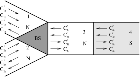
FIG. 8.: Two normal leads (1 and 2) are linked by a semi-transparent beam splitter (BS) and connected to a superconductor (4) via a normal region (3).

C $S$ matrix of the splitter

The beam splitter is described by a $S$ matrix $S_{M}$ which gives the outgoing states as a function of incoming ones. For electrons one obtains:

$$\left(\begin{array}[]{c}c_{1e}^{-}\\ c_{2e}^{-}\\ c_{3e}^{-}\end{array}\right)=S_{M_{e}}\left(\begin{array}[]{c}c_{1e}^{+}\\ c_{2e}^{+}\\ c_{3e}^{+}\end{array}\right)~{}.$$ (102)

Expression of $S_{M_{e}}$ is identical to that of Ref. [33]:

$$S_{M_{e}}=\left(\begin{array}[]{ccc}a&b&\sqrt{\varepsilon}\\ b&a&\sqrt{\varepsilon}\\ \sqrt{\varepsilon}&\sqrt{\varepsilon}&-(a+b)\end{array}\right)~{},$$ (103)

where $a=\left(\sqrt{1-2\varepsilon}-1\right)/2$, $b=\left(\sqrt{1-2\varepsilon}+1\right)/2$, and $\varepsilon$ can vary from 0 to $1/2$. $S_{M_{e}}$ depends only on a single parameter $\varepsilon$ which monitors the transparency of the splitter. For example if $\varepsilon=0$ no transmission occurs from region (1) or (2) to region (3). A similar relation holds for holes:

$$\left(\begin{array}[]{c}c_{1h}^{+}\\ c_{2h}^{+}\\ c_{3h}^{+}\end{array}\right)=S_{M_{h}}\left(\begin{array}[]{c}c_{1h}^{-}\\ c_{2h}^{-}\\ c_{3h}^{-}\end{array}\right)~{}.$$ (104)

Note that the splitter does not couple electrons and holes. Expression of the matrix for holes is given by the relation $S_{M_{h}}(E)=S^{*}_{M_{e}}(-E)$, as no magnetic field is assumed to be present here, but since $S_{M_{e}}$ is real and does not depend on the energy $S_{M_{h}}=S_{M_{e}}$.

D Small biases: Andreev regime

When the applied bias is much smaller than the gap ($eV\ll\Delta$), Andreev reflection between 3 and 4 is the only transmission process. One can then write [34]:

$$\left(\begin{array}[]{c}c_{3e}^{+}\\ c_{3h}^{-}\end{array}\right)=\left(\begin{array}[]{cc}0&\gamma\\ \gamma&0\end{array}\right)\left(\begin{array}[]{c}c_{3e}^{-}\\ c_{3h}^{+}\end{array}\right)~{},$$ (105)

with $\gamma=e^{-i\arccos(E/\Delta)}$. In such a case, all matrix elements like $s_{14pq}$ or $s_{24pq}$ (with $p,q=e,h$) are zero. Setting $x=\sqrt{1-2\varepsilon}$ it is possible to show that:

$$s_{11ee}\!=\!s_{11hh}\!=\!s_{22ee}\!=\!s_{22hh}\! = \!\frac{(x-1)(1+\gamma^{2}x)}{2(1-\gamma^{2}x^{2})}~{},$$ (106)

$$s_{21ee}\!=\!s_{21hh}\!=\!s_{12ee}\!=\!s_{12hh}\! = \!\frac{(x+1)(1-\gamma^{2}x)}{2(1-\gamma^{2}x^{2})}~{},$$ (107)

$$s_{11eh}\!=\!s_{21eh}\! = \!s_{12eh}\!=\!s_{22eh}\!=\!s_{11he}\!=\!s_{21he}\!=\!s_{12he}\!=\!s_{22he}\!$$ (108)

$$= \!\frac{\gamma(1-x)(1+x)}{2(1-\gamma^{2}x^{2})}~{}.$$ (109)

Because $E\ll\Delta$ one can make the assumption that $\gamma\simeq-i$. Since the $S$ matrix elements do not depend on the energy anymore, the integral (101) can be performed. One finally obtains:

$$S_{12}(0)=\frac{2e^{2}}{h}eV\frac{\varepsilon^{2}}{2(1-\varepsilon)^{4}}\left(-\varepsilon^{2}-2\varepsilon+1\right)~{}.$$ (110)

The noise correlations vanish at $\varepsilon=0$, when conductors $1$ and $2$ are equivalent to a two–terminal device decoupled from the superconductor, and in addition, $S_{12}$ vanishes when $\varepsilon=\sqrt{2}-1$. A plot of $S_{12}$ (normalized to the noise in $1$ (or $2$) at $\varepsilon=1/2$) as a function of the beam splitter transmission (figure 9) indicates that indeed, the correlations are positive (bosonic) for $0<\varepsilon<\sqrt{2}-1$ and negative (fermionic) for $\sqrt{2}-1<\epsilon<1/2$. At maximal transmission into the normal leads ($\epsilon=1/2$), the correlations give the negative minimal value: electrons and holes do not interfere and propagate independently into the normal terminals. This is the signature of a purely fermionic system. When the transmission $\epsilon$ is decreased, Cooper pairs may leak in region $3$ because of multiple Andreev processes at the boundary. Further reducing the beam splitter transmission allows to balance the contribution of Cooper pairs with that of normal particles. Expression (110) predicts maximal (positive) correlations at $\epsilon=1/3$: a compromise between a high density of Cooper pairs and weak transmission.

FIG. 9.: Noise correlations between the two normal reservoirs of the device, as a function of transmission of the beam splitter, showing both positive and negative correlations.

E Larger biases

If the applied bias is greater than the gap, transmission of quasi-particles between 3 and 4 is now allowed, and one has to take into account the energy dependence of the $S$ matrix elements. As in section III C, the BTK model is chosen, and thus quasi-particles at arbitrary energy can be handled. For simplicity, the same beam splitter is still used, assuming that its $S$ matrix is independent of the energy. Even though this may appear as a crude approximation, this remains correct for example when the superconductor has a small gap. The $S$ matrix of the whole system is computed in appendix II.

A numerical calculation of noise correlations is performed with the help of Eq. (101). If one considers a high transparency barrier ($Z=0.1$) and a small bias, one finds a good agreement with previous analytical results (figure 10), except that the noise correlations (still normalized to the noise in a normal lead when $\varepsilon=1/2$) do not quite reach the minimal value at $\varepsilon=1/2$. This is an early signature of the potential barrier at the NS interface. The more the bias is increased, the weaker are the positive correlations. If the voltage is large enough (beyond the gap) positive correlations are completely destroyed. As in the analogy with the normal-normal junction encountered previously, Cooper pairs contribute only for a small part to the transport, and the system loses its bosonic features.

FIG. 10.: Noise correlations using an N-S boundary modeled by BTK for a high transparency barrier ($Z=0.1$). From top to bottom, $eV/\Delta=0.5,0.95,1.2,1.8$.

Intermediate transparencies are now considered ($Z=1$, figure 11), and a strikingly different behavior is obtained. For weak biases, noise correlations remain positive over the whole range of $\varepsilon$. It is possible to find an appropriate value (for example $eV=0.95\Delta$) in order to observe oscillations between positive and negative values of the correlations. Further increasing bias, correlations again become negative over the whole range of $\varepsilon$. Calculations for larger values of $Z$ confirm the tendency of the system towards dominant positive correlations at low biases with $S_{12}(\epsilon)/S_{1}(1/2)>1$ over a wide range of $\epsilon$ (not shown). The phenomenon of positive correlations in fermionic systems with a superconducting injector is thus enhanced by the barrier opacity at the N-S boundary. Nevertheless, at the same time, for opaque barriers, the absolute magnitude of $S_{1}$ and $S_{12}$ becomes rather small, which limits the possibility of an experimental check in this regime.

FIG. 11.: Noise correlations using an N-S boundary modeled by BTK for intermediate transparency: $Z=1$ (same biases as in Fig. 10).

A suggestion for the experimental device is depicted figure 12. Assume that a high mobility two dimensional electron gas has a rather clean interface with a superconductor [35]. A first point contact ($P_{1}$) close to the interface selects a maximally occupied electron channel. The beam of electrons is incident on a semi–transparent mirror similar to the one used in the Hanbury–Brown and Twiss fermion analogs [5, 6]. A second point contact located in front of the mirror ($P_{2}$) allows to modulate the reflection of the splitter in order to monitor both bosonic and fermionic noise correlations. In addition, by choosing a superconductor with a relatively small gap, one could observe the dependence of the correlations on the voltage bias without encountering heating effects in the normal metal.

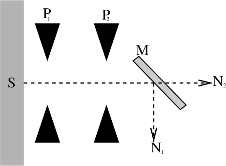
FIG. 12.: Proposed device for the observation of positive/negative correlations; at the boundary of a superconductor ($S$), two point contacts ($P_{1}$) and ($P_{2}$) are connected to a semi-transparent mirror ($M$).

An alternative interpretation of these positive correlation has been proposed [26, 36] in terms of the sign of the effective charges obtained from the spectral weight associated to electrons and holes. Nevertheless, statistical analogies are often useful in condensed matter physics as these allow to isolate the dominant behavior in the transport characteristic of a given system. For instance, in the fractional quantum Hall effect, dissipationless transport occurs because electrons with an odd number of flux quanta represent a composite boson [37].

V Conclusion

Both dynamical and statistical aspects of noise have been presented in a unified formalism. Expressions for the finite-frequency noise and the noise correlations for a conductor containing an arbitrary number of terminals, connected to a superconductor (Eq. (57) and (59)) have been derived. In a first step, a single N-S junction was considered. In the Andreev regime, the noise spectral density presents a singularity at the Josephson frequency, and vanishes beyond. This can be interpreted in terms of an effective charge $2e$ transfered at the boundary. Note that this argument fails if the bias voltage is increased above the gap. In this case, both a single and a double charge transfer are allowed. Thus the effective charges which are identified in the spectral noise density plots are not well defined ($e<e^{*}<2e$).

The non-stationary Aharonov-Bohm effect has been proposed as a tool to analyze these features in a zero frequency measurement. It allows the observation of peaks in the second derivative of the noise with respect to the voltage when the frequency of the applied perturbation is commensurate with the Josephson frequency. Because these kinds of measurements are in principle easier to achieve, this non-stationary Aharonov-Bohm effect has caught the interest of experimentalists [10, 17], who have provided a confirmation of the theoretical predictions of this paper. Thus, a single N-S junction is an adequate system to observe the Josephson frequency with only one superconductor instead of two, as in the usual Josephson effect.

In a second step, the feasibility of an analog to the fermionic Hanbury–Brown and Twiss experiment with a superconductor has been addressed. Correlations are shown to be either positive or negative, depending on the reflection coefficient of the beam splitter. Therefore, such a fermionic system can exhibit a bosonic behavior. A qualitative interpretation of this puzzling result is reached as follows: when the transmission at the interface decreases, Cooper pairs leak on the normal side, and these can be considered as “composite bosons”, hence the positive statistical signature. Recent experiments in the “normal” fermionic Hanbury–Brown and Twiss analog [5, 6] were performed successfully, and these experiments could possibly be extended to the case presented here, giving the opportunity to observe for the first time positive correlations in a fermionic system.

Nevertheless, the issues of this paper present some limitations. All the calculations have been performed in the single channel case, even if a generalization to several channels is possible. However, this extension should not bring major changes. The assumption that the $S$ matrix elements are independent on the energy is correct as long as the applied bias remains small enough. For larger biases, the BTK model takes this energy dependence into account, but only allows numerical calculations. Moreover, further increasing the bias leads to a non-equilibrium situation which cannot be described with this formalism. An appropriate approach would be to employ the Keldysh Green’s functions method. However, in order to go further than the present calculations, heating effects should be taken into account self-consistently. Nevertheless, the physics presented here is rather robust, and different results, especially concerning the effective charge $2e$ in the Andreev regime are not expected. The calculations have been performed for a arbitrary $S$-matrix describing a specific sample, but as pointed out in Ref. [17], all these results can be extended to the diffusive case without difficulty by averaging over the transmission channels with the standard methods of Ref. [38].

Future considerations may include the transport characteristics of other types of superconductors (high $T_{c}$ superconductors), where the gap varies in momentum space. Recently, the noise in a junction between a normal metal and a $d$-wave superconductor has been calculated [39]. Moreover, as it was emphasized above, the study of the statistics and of the effective charges of quasi-particles is a relevant issue in condensed matter systems. For instance, in the fractional quantum Hall effect, Laughlin’s quasi-particles are supposed to obey fractional statistics [40]. Results concerning particles which obey exclusion statistics [41] showed that the shot-thermal noise crossover deviates from the fermion case [42]. Another example is the study of the transport properties of “atomic” composite fermions/bosons, such as alkali atoms or ${}^{3}\mbox{He}$ and ${}^{4}\mbox{He}$ which off-equilibrium properties are not known at this time. Finally, noise correlations have been computed here only at zero frequency. Is there anything to gain from the finite frequency spectrum of noise correlations ? This quantity combines the dynamical aspects of current fluctuations with the statistical nature of multi-terminal geometries.

A $S$ matrix elements of N-S junction with a barrier

Following the BTK model [29], with the barrier potential $V_{B}(x)=V_{B}\delta(x)$ and the pair potential $\Delta(x)=\Delta\theta(x)$, the Bogolubov-de Gennes equations are solved on each side of the junction, giving the states in the normal lead and in the superconductor. The wave functions are continuous at the N-S boundary. Integrating the Bogolubov-de Gennes equations on each side of the junction gives another condition over the derivatives of the wave functions. Writing these conditions for both particle types and both sides of the junction, one obtains four linear systems of equations with four unknowns, which are the $S$ matrix elements:

$$s_{NNee} = s_{SSee}=\displaystyle-\frac{(u_{0}^{2}-v_{0}^{2})(Z^{2}+iZ)}{\gamma}$$ (A1)

$$s_{NNhh} = s_{SShh}=\displaystyle-\frac{(u_{0}^{2}-v_{0}^{2})(Z^{2}-iZ)}{\gamma}$$ (A2)

$$s_{NNhe} = s_{NNeh}=-s_{SShe}=-s_{SSeh}=\displaystyle\frac{u_{0}v_{0}}{\gamma}$$ (A3)

$$s_{SNee} = s_{NSee}=\displaystyle\frac{u_{0}\sqrt{u_{0}^{2}-v_{0}^{2}}(1-iZ)}{\gamma}$$ (A4)

$$s_{SNhh} = s_{NShh}=\displaystyle\frac{u_{0}\sqrt{u_{0}^{2}-v_{0}^{2}}(1+iZ)}{\gamma}$$ (A5)

$$s_{SNhe} = -s_{SNeh}=-s_{NShe}=s_{NSeh}$$ (A6)

$$= \displaystyle\frac{iv_{0}\sqrt{u_{0}^{2}-v_{0}^{2}}Z}{\gamma}~{},$$ (A7)

where:

$$u_{0}^{2}=\frac{1}{2}\left(1+\frac{(E^{2}-\Delta^{2})^{1/2}}{E}\right)=1-v_{0}^{2}~{}.$$ (A8)

$Z=mV_{B}/(\hbar^{2}k_{F})$ is the relative height of the barrier and $\gamma\equiv u_{0}^{2}+(u_{0}^{2}-v_{0}^{2})Z^{2}$. Note that the unitarity of the $S$ matrix is satisfied.

II $S$ matrix elements of a three terminal N-S junction with a barrier

To compute the complete $S$ matrix, one searches which outgoing states are obtained when a single particle is injected in a given terminal. For example, injecting an electron in 4 (ie a state $c^{+}_{4e}$), one obtains reflected waves ($c^{-}_{4e}$ and $c^{+}_{4h}$) and transmitted waves ($c^{-}_{1e}$, $c^{+}_{1h}$, $c^{-}_{2e}$ and $c^{+}_{2h}$) (see Fig. 8). One can therefore deduct the corresponding $S$ matrix elements: $s_{44ee}$, $s_{44he}$ $s_{14ee}$, $s_{14he}$, $s_{24ee}$ and $s_{24he}$. This operation is made for all the terminals and for both types of particle. One obtains:

$$\left(\begin{array}[]{cc}s_{44ee}&s_{44eh}\\ s_{44he}&s_{44hh}\end{array}\right) = S_{SS}-(a+b)S_{SN}\left[1+(a+b)S_{NN}\right]^{-1}S_{NS}~{},$$ (3)

$$\left(\begin{array}[]{cc}s_{14ee}&s_{14eh}\\ s_{14he}&s_{14hh}\end{array}\right) = \left(\begin{array}[]{cc}s_{24ee}&s_{24eh}\\ s_{24he}&s_{24hh}\end{array}\right)=\sqrt{\varepsilon}\Bigl{(}S_{NS}-(a+b)S_{NN}\left[1+(a+b)S_{NN}\right]^{-1}S_{NS}\Bigr{)}~{},$$ (8)

$$\left(\begin{array}[]{cc}s_{41ee}&s_{41eh}\\ s_{41he}&s_{41hh}\end{array}\right) = \left(\begin{array}[]{cc}s_{42ee}&s_{42eh}\\ s_{42he}&s_{42hh}\end{array}\right)=\sqrt{\varepsilon}\,S_{SN}\left[1+(a+b)S_{NN}\right]^{-1}~{},$$ (13)

$$\left(\begin{array}[]{c}s_{11ee}\\ s_{11he}\end{array}\right) = \left(\begin{array}[]{c}s_{22ee}\\ s_{22he}\end{array}\right)=\left[\left(\begin{array}[]{cc}a&0\\ 0&0\end{array}\right)+\left(\begin{array}[]{cc}\varepsilon+a(a+b)&0\\ 0&\varepsilon\end{array}\right)S_{NN}\right]\left[1+(a+b)S_{NN}\right]^{-1}\left(\begin{array}[]{c}1\\ 0\end{array}\right)~{},$$ (24)

$$\left(\begin{array}[]{c}s_{11ee}\\ s_{11he}\end{array}\right) = \left(\begin{array}[]{c}s_{22ee}\\ s_{22he}\end{array}\right)=\left[\left(\begin{array}[]{cc}0&0\\ 0&a\end{array}\right)+\left(\begin{array}[]{cc}\varepsilon&0\\ 0&\varepsilon+a(a+b)\end{array}\right)S_{NN}\right]\left[1+(a+b)S_{NN}\right]^{-1}\left(\begin{array}[]{c}0\\ 1\end{array}\right)~{},$$ (35)

$$\left(\begin{array}[]{cc}s_{12ee}&s_{12eh}\\ s_{12he}&s_{12hh}\end{array}\right) = \left(\begin{array}[]{cc}s_{21ee}&s_{21eh}\\ s_{21he}&s_{21hh}\end{array}\right)=\left(\begin{array}[]{cc}s_{11ee}+1&s_{11eh}\\ s_{11he}&s_{11hh}+1\end{array}\right)~{}.$$ (42)

Here $S_{NS}$, $S_{SN}$, $S_{NN}$ and $S_{SS}$ are $2\times 2$ matrices of which elements have been computed in appendix A. All the calculations have been made above the gap. But the obtained results are valid even if the energy is smaller than the gap, using the correct values for the $S$ matrix of the N-S junction: $S_{NS}$ and $S_{SN}$ are zero, and $S_{NN}$ and $S_{SS}$ are given in appendix A. In this case, expressions of $S_{11}$, $S_{22}$, $S_{21}$ et $S_{12}$ remain the same, but $S_{41}$, $S_{42}$, $S_{14}$ and $S_{24}$ are zero, and $S_{42}=S_{SS}$.

REFERENCES

- [1] L. Saminadayar, D. C. Glattli, Y. Jin, and B. Etienne, Phys. Rev. Lett. 79, 2526 (1997); R. de-Picciotto, M. Reznikov, M. Heiblum, V. Umansky, G. Bunin, and D. Mahalu, Nature 389, 162 (1997).
- [2] R. Hanbury–Brown and Q. R. Twiss, Nature 177, 27 (1956).
- [3] Th. Martin and R. Landauer, Phys. Rev. B 45, 1742 (1992).
- [4] M. Büttiker, Phys. Rev. B 45, 3807 (1992).
- [5] M. Henny et al., Science 284, 296 (1999).
- [6] W. Oliver et al., Science 284, 299 (1999).
- [7] S. R. Yang, Sol. State Commun. 81, 375 (1992); G. B. Lesovik, JETP Lett. 70, 208 (1999).
- [8] R. J. Schoellkopf, P. J. Burke, A. A. Kozhevnikov, D. E. Prober and M. J. Rooks, Phys. Rev. Lett. 78, 3370 (1997).
- [9] G. B. Lesovik and L. S. Levitov, Phys. Rev. Lett. 72, 724 (1994).
- [10] R. J. Schoellkopf, A. A. Kozhevnikov, D. E. Prober and M. J. Rooks, Phys. Rev. Lett. 80, 2437 (1998).
- [11] A. F. Andreev, J. Exp. Theor. Phys. 46, 1823 (1964) [Sov. Phys. JETP 19, 1228 (1964)].
- [12] G. B. Lesovik, T. Martin and J. Torrès, Phys. Rev. B 60, 11935 (1999).
- [13] V. A. Khlus, Zh. Eksp. Teor. Fiz. 93, 2179 (1987) [Sov. Phys. JETP 66, 1243 (1987)].
- [14] M. J. M. de Jong and C. W. J. Beenakker, Phys. Rev. B 49, 16070 (1994); B. A. Muzykantskii and D. E. Khmelnitskii, ibid. 50, 3982 (1994).
- [15] Th. Martin, Phys. Lett. A 220, 137 (1996).
- [16] X. Jehl, P. Payet-Burin, C. Baraduc, R. Calemczuk, and M. Sanquer, Phys. Rev. Lett. 83, 1660 (1999); X. Jehl, M. Sanquer, R. Calemczuk and D. Mailly, (preprint 2000).
- [17] A. A. Kozhevnikov, R. J. Shoelkopf and D. E. Prober, submitted to Phys. Rev. Lett. (1999).
- [18] J. Torrès and T. Martin, Eur. Phys. J. B 12, 319 (1999).
- [19] M. P. Anantram and S. Datta, Phys. Rev. B 53, 16 390 (1996).
- [20] R. Landauer, Philos. Mag. 21, 863 (1970).
- [21] M. Büttiker, Y. Imry, R. Landauer and S. Pinhas, Phys. Rev. B 31, 6207 (1985)
- [22] Y. Imry, Directions in Condensed Matter Physics, edited by G. Grinstein and G. Mazenko (World Scientific, Singapore, 1986).
- [23] S. Datta, Electronic Transport in Mesoscopic Systems, (Cambridge University Press, 1995).
- [24] N. N. Bogolubov, V. V. Tolmachev and D. V. Shirkov, A New Method in the Theory of Superconductivity (Consultant Bureau, New York, 1959); P. G. de Gennes, Superconductivity of Metals and Alloys, (Addison Wesley, 1966, 1989).
- [25] S. Datta, P. Bagwell and M. P. Anantram, Phys. Low-Dim. Struct. 3, 1 (1996).
- [26] Ya. M. Blanter and M. Büttiker, Phys. Rep. 336, 1-2 (2000).
- [27] B. D. Josephson, Phys. Rev. Lett. 1, 251 (1962).
- [28] A. I. Larkin and Yu. N. Ovchinnikov, Sov. Phys. JETP 26, 1219 (1968).
- [29] G. E. Blonder, M. Tinkham and T. M. Klapwijk, Phys. Rev. B 25, 4515 (1982).
- [30] H. Courtois, Ph. Gandit, D. Mailly and B. Pannetier, Phys. Rev. Lett. 76, 130 (1996).
- [31] V. T. Petrashov and V. N. Antonov, JETP Lett. 54, 241 (1991); V. T. Petrashov, V. N. Antonov, P. Delsing and R. Claeson, Phys. Rev. Lett. 70, 347 (1993); ibid. 74, 5268 (1995).
- [32] B. J. van Wees, P. de Vries, P. Magnée and T. M. Klapwijk, Phys. Rev. Lett. 69, 510 (1992); P. H. C. Magnée, N. van der Post, P. H. M. Kooistra, B. J. van Wees and T. M. Klapwijk, Phys. Rev. B 50, 4594 (1994).
- [33] Y. Gefen, Y. Imry and M. Ya. Azbel, Phys. Rev. Lett. 52, 129 (1984); M. Büttiker, Y. Imry and M. Ya. Azbel, Phys. Rev. A, 30, 1982 (1984).
- [34] C. W. J. Beenakker, in Mesoscopic Quantum Physics, eds. E. Akkermans et al., p. 279 (Les Houches LXI, North Holland 1995).
- [35] A. Dimoulas, et al., Phys. Rev. Lett 74, 602 (1995).
- [36] T. Gramespacher and M. Büttiker, Phys. Rev. B 61, 8125 (2000).
- [37] see for example A. H. MacDonald, in Mesoscopic Quantum Physics, eds. E. Akkermans et al., p. 279 (Les Houches LXI, North Holland 1995).
- [38] C. W. J. Beenakker, Review of Modern Phys. 69/3, 731 (1997).
- [39] J.-X. Zhu and C. S. Ting, Phys. Rev. B 59, R14165 (1999); ibid. 61, 1456 (2000).
- [40] F. D. M. Haldane, Phys. Rev. Lett. 66, 1529 (1991).
- [41] F. D. M. Haldane, Phys. Rev. Lett. 67, 937 (1991).
- [42] S. B. Isakov, Th. Martin and S. Ouvry, Phys. Rev. Lett. 83, 580 (1999).