Renormalization of spectral lineshape and dispersion below $T_{c}$ in Bi₂Sr₂CaCu₂O_8+δ

Abstract

Angle-resolved photoemission (ARPES) data in the superconducting state of Bi₂Sr₂CaCu₂O_8+δ show a kink in the dispersion along the zone diagonal, which is related via a Kramers-Krönig analysis to a drop in the low-energy scattering rate. As one moves towards $(\pi,0)$, this kink evolves into a spectral dip. The occurrence of these anomalies in the dispersion and lineshape throughout the zone indicate the presence of a new energy scale in the superconducting state.

The high temperature superconductors exhibit many unusual properties, one of the most striking being the linear temperature dependence of the normal state resistivity. This behavior has been attributed to the presence of a quantum critical point, where the only relevant energy scale is the temperature[1]. However, new energy scales become manifest below $T_{c}$ due to the appearance of the superconducting gap and resulting collective excitations. The effect of these new scales on the ARPES spectral function below $T_{c}$ have been well studied near the $(\pi,0)$ point of the zone [2, 3]. In this Letter we show how these scales manifest themselves in the spectral functions over the entire Brillouin zone.

Remarkably, we find that these effects are manifest even on the zone diagonal where the gap vanishes, with significant changes in both the spectral lineshape and dispersion below $T_{c}$, relative to the normal state (where the nodal points exhibit quantum critical scaling [4]). Specifically, below $T_{c}$ a kink in the dispersion develops along the diagonal at a finite energy ($\sim$70 meV). This is accompanied, as required by Kramers-Krönig relations, by a reduction in the linewidth leading to well-defined quasiparticles. As one moves away from the node, the renormalization increases, and the kink in dispersion along the diagonal smoothly evolves into the spectral dip [2], with the same characteristic energy scale throughout the zone. We suggest that a natural interpretation of all of these spectral renormalizations is in terms of the electron interacting with a collective excitation below $T_{c}$, which is likely that seen directly by neutron scattering [5].

We begin our analysis by recalling [6] that, within the impulse approximation, the ARPES intensity for a quasi-two-dimensional system is given by [7] $I({\bf k},\omega)=I_{0}({\bf k})f(\omega)A({\bf k},\omega)$. Here ${\bf k}$ is the in-plane momentum, $\omega$ is the energy of the initial state relative to the chemical potential, $f$ is the Fermi function, $I_{0}$ is proportional to the dipole matrix element $\left|M_{fi}\right|^{2}$, and $A$ is the one-particle spectral function. Fig. 1 shows data [8] as a function of ${\bf k}$ and $\omega$.

FIG. 1.: (a) The ARPES intensity as a function of ${\bf k}$ and $\omega$ at $h\nu$=22eV and T=40K. MB is the main band, and SL a superlattice image. (b) A constant $\omega$ cut (MDC) from (a). (c) A constant ${\bf k}$ cut (EDC) from (a). The diagonal line in the zone inset shows the location of the ${\bf k}$ cut; the curved line is the Fermi surface.

$A({\bf k},\omega)=(-1/\pi)\Im mG({\bf k},\omega+i0^{+})$ can be written as

$$A({\bf k},\omega)={1\over\pi}{{\left|{\Sigma^{\prime\prime}({\bf k},\omega)}\right|}\over{\left[{\omega-\epsilon_{{\bf k}}-\Sigma^{\prime}({\bf k},\omega)}\right]^{2}+\left[{\Sigma^{\prime\prime}({\bf k},\omega)}\right]^{2}}}.$$ (1)

where the self-energy $\Sigma=\Sigma^{\prime}+i\Sigma^{\prime\prime}$ and $\epsilon_{{\bf k}}$ is the bare dispersion. For ${\bf k}$ near $k_{F}$, and varying normal to the Fermi surface (shown in the inset in Fig. 1), we may write $\epsilon_{{\bf k}}\simeq v_{F}^{0}(k-k_{F})$, where both $k_{F}(\theta)$ and the bare Fermi velocity $v_{F}^{0}(\theta)$ depend in general on the angle $\theta$ along the Fermi surface.

In Fig. 2a, we plot the dispersion of the spectral peak above $T_{c}$ obtained from constant ${\bf k}$ scans (energy distribution curves or EDCs), and the peak in momentum obtained from constant $\omega$ scans (momentum distribution curves or MDCs) [4] from data similar to Fig. 1. We find that the EDC and MDC peak dispersions are very different, a consequence of the $\omega$ dependence of $\Sigma$. To see this, we note from Eq. (1) that the MDC at fixed $\omega$ is a Lorentzian centered at $k=k_{F}+\left[\omega-\Sigma^{\prime}(\omega)\right]/v_{F}^{0}$, with a width (HWHM) $W_{M}=|\Sigma^{\prime\prime}(\omega)|/v_{F}^{0}$, provided (i) $\Sigma$ is essentially independent [9] of $k$ normal to the Fermi surface, and (ii) the dipole matrix elements do not vary significantly with $k$ over the range of interest. That these two conditions are fulfilled can be seen by the nearly Lorentzian MDC lineshape of the data in Fig. 1b.

On the other hand, in general, the EDC at fixed ${\bf k}$ (Fig. 1c) has a non-Lorentzian lineshape reflecting the non-trivial $\omega$-dependence of $\Sigma$, in addition to the Fermi cutoff at low energies. Thus the EDC peak is not given by $\left[\omega-v_{F}^{0}(k-k_{F})-\Sigma^{\prime}(\omega)\right]=0$ but also involves $\Sigma^{\prime\prime}$, unlike the MDC peak. Further, if the EDC peak is sharp enough, making a Taylor expansion we find that its width (HWHM) is given by $W_{E}\simeq|\Sigma^{\prime\prime}(E_{k})|/[1-\partial\Sigma^{\prime}/\partial\omega|_{E_{k}}]$, where $E_{k}$ is the peak position.

We see that it is much simpler to interpret the MDC peak positions, and thus focus on the change in the MDC dispersion going from the normal (N) to the superconducting (SC) state shown in Fig. 2b. The striking feature of Fig. 2b is the development of a kink in the dispersion below $T_{c}$. At fixed $\omega$ let the dispersion change from $k_{N}$ to $k_{SC}$. Using $v_{F}^{0}(k_{N}-k_{SC})=\Sigma_{SC}^{\prime}(\omega)-\Sigma_{N}^{\prime}(\omega)$, we directly obtain the change in real part of $\Sigma$ plotted in Fig. 2c. The Kramers-Krönig transformation of $\Sigma_{SC}^{\prime}-\Sigma_{N}^{\prime}$ then yields $\Sigma_{N}^{\prime\prime}-\Sigma_{SC}^{\prime\prime}$, plotted in Fig. 2d, which shows that $|\Sigma_{SC}^{\prime\prime}|$ is smaller than $|\Sigma_{N}^{\prime\prime}|$ at low energies.

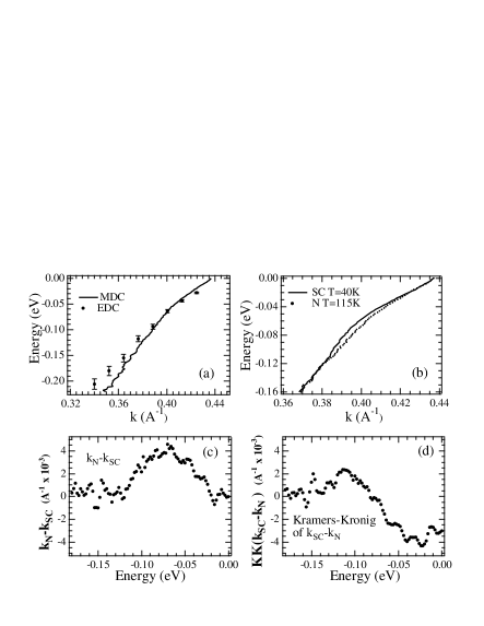
FIG. 2.: ARPES data along the $(\pi,\pi)$ direction at $h\nu$=28eV. (a) EDC dispersion in the normal state compared to the MDC dispersion. The EDCs are shown in Fig. 3d. (b) MDC dispersions in the superconducting state (T=40K) and normal state (T=115K). (c) change in MDC dispersion from (b). (d) Kramers-Krönig transform of (c).

We compare these results in Fig. 3a with the $W_{M}=|\Sigma^{\prime\prime}|/v_{F}^{0}$ estimated directly from the MDC Lorentzian linewidths. The normal state curve was obtained from a linear fit to the corresponding MDC width data points in Fig. 3a, and then the data from Fig. 2d was added to it to generate the low temperature curve. We are thus able to make a quantitative connection between the appearance of a kink in the (MDC) dispersion below $T_{c}$ and a drop in the low energy scattering rate in the SC state relative to the normal state, which leads to the appearance of quasiparticles below $T_{c}$ [10]. We emphasize that we have estimated these $T$-dependent changes in the complex self-energy without making fits to the EDC lineshape, thus avoiding the problem of modeling the $\omega$ dependence of $\Sigma$ and the extrinsic background.

In Fig. 3b, we plot the EDC width obtained as explained in [10] from Fig. 3d. As an interesting exercise, we present in Fig. 3c the ratio of this EDC width to the MDC width of Fig. 3a (dotted lines), and compare it to the renormalized MDC velocities, $1/v\equiv dk/d\omega$, obtained directly by numerical differentiation of Fig. 2b (solid lines). We note that only for a sufficiently narrow EDC lineshape is the ratio $W_{E}/W_{M}\simeq v_{F}^{0}/[1-\partial\Sigma^{\prime}/\partial\omega]=v_{F}$. Interestingly, only in the SC state below the kink energy do these two quantities agree, which implies that only in this case does one have a Fermi liquid.

Similar kinks in the dispersion have been seen by ARPES in normal metals due to the electron-phonon interaction[11]. Phonons cannot be the cause here, since our kink disappears above $T_{c}$. Rather, our effect is suggestive of coupling to an electronic collective excitation which only appears below $T_{c}$.

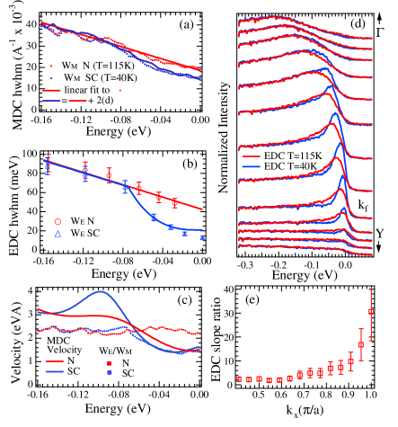
FIG. 3.: (a) Comparison of change in $\Sigma^{\prime\prime}$ obtained directly from the MDC widths (HWHM) to the one obtained from the dispersion in Fig. 2d by using the Kramers-Krönig transform. (b) HWHM width obtained from EDCs shown in (d). Lines marked by fit are linear in normal state and linear/cubic in superconducting state. The data in (b) fall below the fits at low energies because of the Fermi cut-off of the EDCs. (c) Renormalized MDC velocity obtained from differentiating Fig. 2b (solid lines), compared to the ratio $W_{E}/W_{M}$ from (a) and (b). (e) Ratio of EDC dispersion slopes above and below the kink energy at various points along the Fermi surface (from middle panels of Fig. 4).

We now study how the lineshape and dispersion evolve as we move along the Fermi surface. Away from the node a quantitative analysis (like the one above) becomes more complicated [12] and will be presented in a later publication. Here, we will simply present the data. In Fig. 4, we plot raw (2D) data as obtained from our detector for a series of cuts parallel to the $MY$ direction (normal state in left panels, superconducting state in middle panels). We start from the bottom row that corresponds to a cut close to the node and reveals the same kink described above. As we move towards $(\pi,0)$, the dispersion kink (middle panels) becomes more pronounced and at around $k_{x}$=0.55 develops into a break separating the faster dispersing high energy part of the spectrum from the slower dispersing low energy part. This break leads to the appearance of two features in the EDCs, shown in the right panels of Fig. 4. Further towards $(\pi,0)$, the low energy feature, the quasiparticle peak, becomes almost dispersionless. At the $(\pi,0)$ point, this break effect becomes the most pronounced, giving rise to the well known peak/dip/hump [2] in the EDC. We note that there is a continuous evolution in the zone from kink to break, and these features all occur at exactly the same energy.

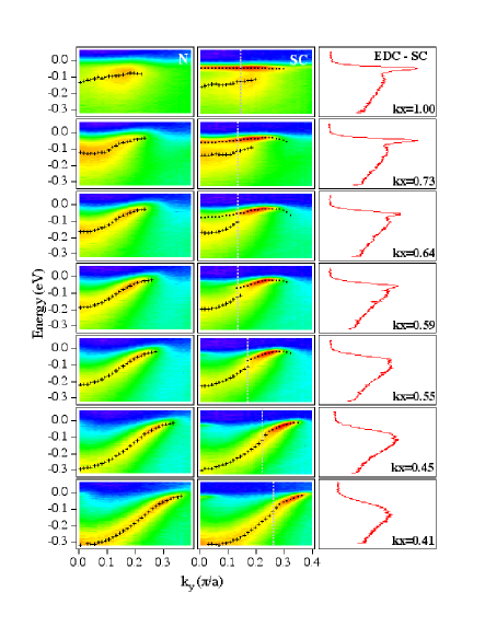
FIG. 4.: Left panels: Log of normal state ($h\nu$=22eV, T=140K) ARPES intensity along selected cuts parallel to $MY$. (shown in zone inset in Fig. 1). EDC peak positions are indicated by crosses. Middle panels: Log of superconducting state (T=40K) intensity at the same cuts as for left panels. Crosses indicate positions of broad high energy peaks, dots sharp low energy peaks. Right panels: EDCs at locations marked by the vertical lines in the middle panels.

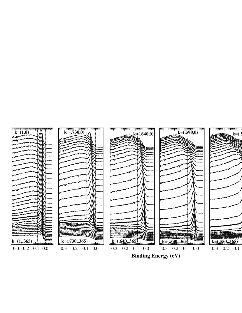
FIG. 5.: ARPES intensity (T=40K) along selected cuts from Fig. 4. The thick lined curves correspond approximately to ${\bf k}_{F}$. Vertical lines are at 0 and -80 meV.

The above evolution is suggestive of the self-energy becoming stronger as the $(\pi,0)$ point is approached. This can be quantified from the observed change in the dispersion. In Fig. 3(e) we plot the ratio of the EDC dispersion slope above and below the kink energy at various points along the Fermi surface obtained from middle panels of Fig. 4. Near the node, this ratio is around 2, but becomes large near the $(\pi,0)$ point because of the nearly dispersionless quasiparticle peak[2].

The lineshape also indicates that the self-energy is larger near $(\pi,0)$, as is evident in Fig. 5. Along the diagonal, there is a gentle reduction in $\Sigma^{\prime\prime}$ at low energies, as shown in Fig. 3 (a) and (b), with an onset at the dispersion kink energy scale. In contrast, near the $(\pi,0)$ point there must be a very rapid change in $\Sigma^{\prime\prime}$ in order to produce a spectral dip, as quantified in Refs. [2, 13]. Despite these differences, it is important to note that these changes take place throughout the zone at the same characteristic energy scale (vertical line in Fig. 5).

As discussed in Ref. [2] the near-$(\pi,0)$ ARPES spectra can be naturally explained in terms of the interaction of the electron with a collective mode of electronic origin which only exists below $T_{c}$. It was further speculated that this mode was the neutron resonance [5], an interpretation which received further support from Ref. [3] where the doping dependence of ARPES spectra were examined. Here we have shown that dispersion and lineshape anomalies have a continuous evolution throughout the zone and are characterized by a single energy scale. This leads us to suggest that the same electron-mode interaction determines the superconducting lineshape and dispersion at all points in the zone, including the nodal direction [14]. In essence, there is a suppression of the low energy scattering rate below the finite energy of the mode. Of course, since the neutron mode is characterized by a $(\pi,\pi)$ wavevector, one would expect its effect on the lineshape to be much stronger at points in the zone which are spanned by $(\pi,\pi)$ [15], as observed here.

In summary, we have shown by a simple, self-consistent analysis based on general properties of the spectral function and self-energy, that Bi₂Sr₂CaCu₂O_8+δ shows a dispersion renormalization along the zone diagonal which is directly related to a drop in the low energy scattering rate below $T_{c}$. The anomalies in the dispersion and lineshape evolve smoothly as one moves from the zone diagonal to the zone corner, but always show the same characteristic energy scale. We suggest that this suppression of the scattering rate below $T_{c}$ at all points in the Brillouin zone is due to the presence of a gap and a finite energy collective mode, which we identify with the magnetic resonance observed by neutron scattering.

MR would like to thank P.D. Johnson for discussions. This work was supported by the NSF DMR 9974401, the U.S. DOE, Basic Energy Sciences, under contract W-31-109-ENG-38, the CREST of JST, and the Ministry of Education, Science, and Culture of Japan. The Synchrotron Radiation Center is supported by NSF DMR 9212658. JM is supported by the Swiss National Science Foundation, and MR in part by the Indian DST through the Swarnajayanti scheme.

Note added: After completion of this work, we became aware of related work by Bogdanov et al., cond-mat/0004349.

REFERENCES

- [1] B. Batlogg and C. M. Varma, Physics World, Feb., p. 33 (2000).
- [2] M. R. Norman et al., Phys. Rev. Lett. 79, 3506 (1997); M. R. Norman and H. Ding, Phys. Rev. B 57, R11089 (1998).
- [3] J.C. Campuzano et al., Phys. Rev. Lett. 83, 3709 (1999).
- [4] T. Valla et al., Science 285, 2110 (1999).
- [5] H. F. Fong et al., Nature 398, 588 (1999).
- [6] M. Randeria et al., Phys. Rev. Lett. 74, 4951 (1995).
- [7] The experimental signal is a convolution of this with the energy resolution and a sum over the momentum window, plus an additive (extrinsic) background.
- [8] The optimally doped Bi2Sr2CaCu2O8+δ(=90K) samples, grown using the floating zone method, were mounted with either or parallel to the photon polarization, and cleaved in situ at pressures less than 510-11 Torr. Measurements were carried out at the Synchrotron Radiation Center in Madison WI, on the U1 undulator beamline supplying photons/sec, using a Scienta SES 200 electron analyzer with energy resolution of 16 meV and a -resolution of 0.0097 .
- [9] Note that: (1) a linear dependence of on can be absorbed into the definition of ; (2) has an implicit dependence on .
- [10] A. Kaminski et al., Phys. Rev. Lett. 84, 1788 (2000).
- [11] M. Hengsberger et al., Phys. Rev. Lett. 83, 592 (1999); T. Valla et al., ibid., 2085 (1999).
- [12] Such an analysis would need to include (1) the superconducting gap which affects through a pairing contribution; (2) the quadratic dispersion about the symmetry line, which is close to near .
- [13] M. R. Norman et al., Phys. Rev. B 60, 7585 (1999).
- [14] M. Eschrig and M. R. Norman, cond-mat/0005390.
- [15] Z.-X. Shen and J. R. Schrieffer, Phys. Rev. Lett. 78, 1771 (1997).