Roughness of fracture surfaces

Abstract

We study the roughness of fracture surfaces of three dimensional samples through numerical simulations of a model for quasi-static cracks known as Born Model. We find for the roughness exponent a value $\zeta\simeq 0.5$ measured for “small length scales” in microfracturing experiments. Our simulations confirm that at small length scales the fracture can be considered as quasi-static. The isotropy of the roughness exponent on the crack surface is also showed. Finally, considering the crack front, we compute the roughness exponents of longitudinal and transverse fluctuations of the crack line ($\zeta_{\|}\sim\zeta_{\perp}\sim 0.5$). They result in agreement with experimental data, and support the possible application of the model of line depinning in the case of long-range interactions.

A large amount of studies has been devoted to the problem of material strength and to the study of fractures in disordered media [1, 2]. In this paper we focus our attention on the self-affine properties of the fracture surface [3, 4]. By self-affinity one means that the surface coordinate $z$ in the direction perpendicular to the crack or fracture (x-y) plane has the following scaling properties:

$$\begin{array}[]{rrr}z(\lambda x,y)&=&\lambda^{\zeta_{x}}z(x,y)\\ z(x,\lambda y)&=&\lambda^{\zeta_{y}}z(x,y)\end{array}$$ (1)

where the two $\zeta$ exponents are known as roughness exponents, and the $\hat{y}$ direction is chosen along the direction of propagation of the crack. Even if these two directions seem to play a different role in the morphological description of the fracture surface, experimental measurements showed that these two directions have similar scaling properties for very different materials [5]. A unique roughness exponent is then generally considered (therefore $\zeta_{x}=\zeta_{y}\equiv\zeta$), and it has been claimed that it has a universal value of $\zeta=0.8$ [3]. This behaviour has been confirmed for a large variety of experimental situations [6, 7]. However, more extended studies have also shown that in some experimental conditions, for fracture surfaces of metallic materials, one deals with a different value of $\zeta=0.5$ [8]. These two values of the roughness exponent are connected to the length scale at which the crack is examined. In particular, at small length scales one observes a roughness exponent $\zeta=0.5$, whereas at large length scales the larger value $\zeta=0.8$ is found. These results have recently been connected with the velocity of the crack front [9], and interpreted as a quasi-static regime and a dynamic one: the value of $\zeta=0.5$ should be expected in the quasi-static regime. This connection comes from the suggestion that the crack surface can be thought as the trace left by the crack front [10] so that the problem of the surface roughness can be mapped on the problem of the evolution of a line moving in a random medium. Ertaş and Kardar [11] introduce a couple of non-linear Langevin equations to describe this evolution and their model can be usefully considered to evaluate the statistical properties of the evolution of a crack surface line. In this case, these equations describe longitudinal and transverse fluctuations with respect to the fracture plane containing the line velocity and the pulling force [12]. Values obtained are close to the roughness measured at large length scales. At small length scales however, the crack front behaves as a moving line undergoing a depinning transition, and in this case results from Ertaş and Kardar model [13, 14, 15], should be revised [12] considering long-range interactions, to give [9] $\zeta_{\|}$ and $\zeta_{\perp}$ equal to $0.5$ respectively for longitudinal and transverse fluctuations. Another interesting model has been proposed by Roux et al. [16, 17] where the fracture surface is expected to be a minimal energy surface. In two dimension this problem maps directly in the random directed polymer problem: the polymer with the minimum energy is the collection of the “weakest” monomers in the medium that form a directed path. This corresponds to the surface crack of a fuse model and for brittle fractures gives a roughness exponent $\zeta=2/3$ in 2 dimensions. Similar arguments hold for $d=3$ and are discussed for a scalar model of fracture in [18]. In this case on has $\zeta=0.42\pm 0.01$, differently from experimental results [18].

In this paper we present a numerical study of a fracture propagation for a model of quasi-static fractures to show that in such a regime, the roughness exponent is in agreement with the one found at small length scales. Comparisons with theoretical models are discussed at the end of this work. To model the fracture propagation we use a mesoscopic model known as Born Model (BM), describing the sample through a discrete collection of sites connected by springs [19]. The statistical properties of the two dimensional BM have been previously considered in [20, 21]. In particular for $d=2$ [22] a value of roughness of the fracture surface of $\zeta\simeq 0.64(3)$ in agreement with other measurements [23] has been found. In the BM the elastic energy of the sample under load is given by the energy of deformation for the springs connecting the sites of the sample. The elastic potential energy consists of two different terms, describing, respectively, a central force and a non-central force contribution:

$$V=\frac{1}{2}\sum_{i,j}V_{i,j}=\frac{1}{2}\sum_{i,j}\big{\{}(\alpha-\beta)[({\bf u}_{i}-{\bf u}_{j})\cdot{\bf\hat{r}}_{i,j}]^{2}+\beta[{\bf u}_{i}-{\bf u}_{j}]^{2}\big{\}}$$ (2)

where ${\bf u}_{i}$ is the displacement vector for site $i$, ${\bf\hat{r}}_{i,j}$ is the unit vector between $i$ and $j$, $\alpha$ and $\beta$ are force constants tuning the effects of central and non-central force contributions, and the sum is over the nearest neighbour sites connected by a non-broken spring. By imposing the condition $\nabla_{{\bf u}}V=0$ one obtains a series of equations for the fields ${\bf u}_{i}$. Solving them one obtains the equilibrium positions of the springs in the sample. It has to be noticed that since one is interested in the equilibrium position one has to consider only the ratio of the two parameters $\beta/\alpha$ (hereafter we will consider $\alpha=1$ and a varying $\beta$). Simulations show that varying $\beta$ between $1$ and $0$ corresponds to varying the Poisson coefficient between $0$ and $1/2$, as expected from the theory of elasticity. At this point with a probability proportional to $\sqrt{V_{i,j}}$, which represents a generalized elongation, one selects a spring to remove on the fracture boundary, with the result of obtaining a connected fracture [20, 22]; by doing that the boundary conditions of the system change and one has to compute a new equilibrium position. Breaking a new bond after the complete relaxation of the lattice, results in a slow velocity for the fracturing process, which mimics a quasi-static process.

The elastic springs can be arranged in different kinds of networks: however in two dimensions one has to consider a triangular lattice, for a square lattice does not correctly describe the response of the system to the applied stress. In three dimensions as well, one has to consider a network with the correct response, which results in a more complex arrangement with respect to the case of the simple cube. In our case we chose a sample described by a Face Centered Cubic (FCC) structure and we applied a mode I loading on two opposite faces by fixing their displacement field. We then applied periodic boundary conditions on a second couple of opposite faces and on one of the two remaining faces we put a starting notch (see Fig.1).

             

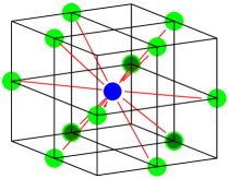
Fig. 1.–: On the left, the setup for the simulation, note the deterministic starting notch. On the right there is the FCC cell with the bonds used in the Born Model.

Starting from this setup we realized different simulations by stopping the algorithm when the sample is divided in two parts. At this point we started considering the surface of the fracture and we analyzed its statistical properties. We performed simulations for different values of the $\beta$ parameter, for 20 different samples of $32\times 32\times 16$ cells (each cell contains 4 sites for a total number of $2^{16}$ sites) for each value of $\beta$, for which we obtained all the relevant results. Further simulations on $40\times 40\times 20$ and $50\times 50\times 25$ FCC cells lattices were performed to verify the generality of the results. Simulations lasted from a minimum of 18-hours of CPU time for each $32\times 32\times 16$ cells lattice, up to more than 180 hours for a $50\times 50\times 25$ cells lattice, on a Digital alpha-station (500 MHz).

An example of a final fracture surface is shown in Fig.2, whereas a typical broken sample is showed in Fig.3: different colors show damaged (with at least one broken bond) and undamaged sites, and the structure of the FCC lattice.

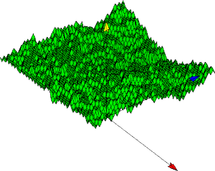
Fig. 2.–: Fracture surface of $64\times 64$ sites, obtained from a sample of $32\times 32\times 16$ FCC cells ($\alpha=1,\beta=1$).

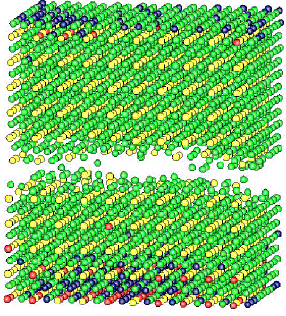
Fig. 3.–: An example of a just broken lattice of $10\times 10\times 10$ FCC cells (4000 sites: 4 site per cell). Here the fracture width has been enhanced for convenience, damaged sites are yellow and green the others are blue and red. The double coloring (yellow/green and blue/red) is supplied to better distinguish FCC cells.

To compute the roughness exponent, we considered different cuts of the fracture surface, some of them along the $\hat{x}$ direction and some of them along the $\hat{y}$ direction which is the direction of propagation of the crack. In principle we did not consider the fracture to be isotropic, but we tried to recover the roughness exponents $\zeta_{x}$ and $\zeta_{y}$. To measure the roughness of the surface, we followed the procedure described in [5], by introducing the two spatial correlation functions

$$\begin{array}[]{rrr}C_{x}(\rho)&=&\langle[z(x_{i}+\rho,y_{i})-z(x_{i},y_{i})]^{2}\rangle\\ C_{y}(\rho)&=&\langle[z(x_{i},y_{i}+\rho)-z(x_{i},y_{i})]^{2}\rangle\end{array}$$ (3)

where the average $\langle...\rangle$ is taken over the different $x$ and $y$ of the sites on the surface, and over different realization of the surfaces. Then we considered the power spectra $\tilde{C}_{x,y}(k)$ of the profile, that is to say we studied the Fourier transform of the previous introduced correlation functions. In this way the boundary effects are considered only in the large $k$ modes [24]. For self-affine profiles these power spectra are expected to scale as

$$\tilde{C}_{x,y}(k)\propto k^{-(1+2\zeta_{x,y})}$$ (4)

Fits for the Fourier transform are shown in Fig.4. Results show that the value of $\zeta_{x}$ is equal within the error bars to the value of $\zeta_{y}$. The two directions on the fracture surface show the same statistical properties as expected for a large variety of materials; the surface can then be described by a unique roughness exponent $\zeta$. Moreover, the value of $\zeta$ does not seem to depend on the value of $\beta$, and is in complete agreement with the value expected for fractures in a quasi-static regime [9]. All the results are summarized in Tab.I.

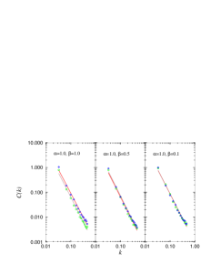
Fig. 4.–: Fourier transforms of the autocorrelation functions for the heights for different values of $\beta$. All the fits have the same slope, which corresponds to a value of $\zeta\sim 0.5$.

FCC cells $\beta$ $\zeta_{x}$ $\zeta_{y}$ $32\times 32\times 16$ $1.0$ $0.50\pm 0.05$ $0.49\pm 0.05$ $0.5$ $0.49\pm 0.06$ $0.46\pm 0.06$ $0.1$ $0.49\pm 0.06$ $0.47\pm 0.05$ $0.01$ $0.48\pm 0.07$ $0.47\pm 0.06$ $40\times 40\times 20$ $1.0$ $0.48\pm 0.07$ $0.47\pm 0.06$ $50\times 50\times 25$ $0.5$ $0.48\pm 0.05$ $0.48\pm 0.05$

Table I.–: Behavior of the two roughness exponents for different values of the $\beta$ parameter, for FCC samples of different sizes.

To test such a measure (as suggested by Ref.[25]) we also studied the scaling behaviour of the surface width in direct space, along cuts perpendicular to the direction of the crack propagation: the same behaviour for $\zeta$ is recovered (see Fig.5). In this case results are quite striking, since a small deviation from the value of 0.5 leads to slightly displaced curves. This observation allows us to be enough confident in these results even if they extend for about one decade.

Fig. 5.–: Behaviour of the width functions: data are collapsed for $\zeta=0.5$, and $z=1.5$. Inset shows the width vs time for increasing sizes of $\Delta$.

An interesting analisys is the computation of the roughness of fluctuations of the crack front, compared with experiments and with the theory of line depinning by Ertaş and Kardar. It has to be noticed that the definition of the crack front has some sort of ambiguity, because during the fracturing process more than one fracturing plane can develop, but just one among these will belong to the final fracture surface. Experimentally, this exponent can be found arresting the fracture during propagation, and injecting indian ink into the cracks under moderate vacuum. Samples are then dried and the process of fracturing is continued until complete separation is reached [12]. From this point of view, one has to look at the border of the fracture belonging to what will be the final surface. Also, this corresponds to considering the fracture as the trace left from the crack front: this therefore belongs to the final surface.

Following this idea, we measured the roughness for the fluctuations of the crack front along the direction parallel to the line velocity ($\zeta_{\|}$) and for those perpendicular to it ($\zeta_{\perp}$), during the crack evolution. In the same way as the experimental one, we mark the sites reached through the fracturing process until a certain timestep. The process then continues up to complete separation. We then look at the marked part of the final surface, to recover the crack front. Final results are from Fourier transform of an average at subsequent steps of the autocorrelation function in the steady state. In either cases we again obtained for both a value close to $0.5$ (see Tab.II), in good agreement with experiments.

FCC cells $\beta$ $\zeta_{\|}$ $\zeta_{\perp}$ $32\times 32\times 16$ $1.0$ $0.51\pm 0.05$ $0.49\pm 0.06$ $0.5$ $0.55\pm 0.05$ $0.48\pm 0.06$ $0.1$ $0.54\pm 0.07$ $0.50\pm 0.07$ $0.01$ $0.54\pm 0.06$ $0.51\pm 0.07$ $40\times 40\times 20$ $1.0$ $0.49\pm 0.05$ $0.49\pm 0.08$ $50\times 50\times 25$ $0.5$ $0.47\pm 0.08$ $0.46\pm 0.09$

Table II.–: Measured values for the roughness of the crack front for different values of $\beta$. $\zeta_{\|}$ and $\zeta_{\perp}$ are respectively the roughness for longitudinal and transverse fluctuations of the crack front. The large error bars for the $50\times 50\times 25$ samples are due to the limited number of sample examined, because of the lasting of simulations.

As regards the roughness exponent we can conclude from our simulations that its value is the one characteristic of the quasi-static evolution of cracks. This result is confirmed by quantitative analysis [26] and is to be compared with results from the different approaches. Our conclusions seem to be different from the conclusions of the directed polymers approach as presented with their scalar problem in [18]. The value of $\zeta=0.42\pm 0.01$ found with this model could be related to the different physics of the fuse networks. The use of this model in fact, comes from the assumption that in two dimensions a fracture can be described by means of a scalar model. This is not stated in three dimensions, where a description like the one that comes from the theory of elasticity can be obtained only through a vectorial model. This could also explain the difference between our results, which agree with experimental values, and those for the fuse network in [27].

The analysis of the roughness of longitudinal and transverse fluctuations of the crack front, give results still in agreement with experiments and seems to confirm the mapping of the crack front to a line undergoing a pinning-depinning transition. Our result is also to be compared with the one from [28]. In this paper in fact it is stated that an explanation of the roughness in terms of a quasi-static fracturing process seems unlikely. This seems to suggest a different conclusion, as in our simulations elastic waves are cut-off through relaxation of the lattice after each bond-breaking. However, fluctuations are still enclosed in the stocastic process for the fracture.

In conclusion we presented numerical simulations of the fracture of a three dimensional sample. Our result supports the idea that the fracture roughness exponent is related to the different length scale at which the sample is analysed and then to the different dynamics of the crack. In particular for short length scales where the fracture can be identified as quasi-static the roughness exponent is $\zeta=0.5$. We also show that for elastic fractures one can expect isotropic behaviour in the developing of the surface: our results show no dependance from the direction on crack surface. As regards the crack front, our results agree with experimental measurements, and support the mapping to line depinning in the case of long-range interactions.

We whish to thank A.Petri and R.C.Ball for useful discussions. We also acknowledge support of EU contract N. ERBFMRXCT980183

References

- [1] H. J. Herrmann and S. Roux, (Ed.), Statistical models for the fracture of disordered media, Elsevier, Amsterdam (1990)
- [2] B.K. Chakrabarti and L.G. Benguigui, Statistical Physics of Fracture and Breakdown in Disordered Systems (Clarendon Press, Oxford, 1997).
- [3] E. Bouchaud, G. Lapasset and J. Planes, Europhys. Lett. 13, 73 (1990).
- [4] B.B. Mandelbrot, D.E. Passoja and A.J. Paullay, Nature (London), 308, 721 (1984).
- [5] F. Plouraboué, P. Kurowski, J.P. Hulin, S. Roux and J. Schmittbuhl, Phys. Rev. E 51, 1675 (1995).
- [6] K.J. Måløy, A. Hansen, K.L. Hinrichsen and S. Roux, Phys. Rev. Lett. 68, 213 (1992).
- [7] J. Schmittbuhl, S. Roux and Y. Berthaud, Europhys. Lett. 28, 585 (1994).
- [8] V.Yu. Milman, R. Blumenfeld, N.A. Stelmashenko and R.C. Ball, Phys. Rev. Lett. 71, 204 (1993).
- [9] P. Daguier, B. Nghiem, E. Bouchaud and F. Creuzet, Phys. Rev. Lett. 78, 1062 (1997).
- [10] J.-P. Bouchaud, E. Bouchaud, G. Lappaset and L. Planès, Phys. Rev. Lett. 71, 2240 (1993).
- [11] D. Ertaş and M. Kardar, Phys. Rev. Lett. 69, 929 (1992), Phys. Rev. E 48, 1228 (1993).
- [12] E. Bouchaud, J. Phys.: Condens. Matter 9, 4319 (1997).
- [13] D. Ertaş and M. Kardar, Phys. Rev. Lett. 73, 1703 (1994), Phys. Rev. B 53, 3520 (1996).
- [14] E. Medina, M. Kardar, Phys. Rev. Lett. 66, 3187 (1991).
- [15] M. Kardar, Y-.C. Zhang, Europhys. Lett. 8, 233 (1989).
- [16] S. Roux and D. François, Scr. Metall. 25, 1092 (1991).
- [17] A. Hansen, E.L. Hinrichsen and S. Roux, Phys. Rev. Lett. 66, 2476 (1991).
- [18] V. I. Raisanen, E. T. Seppala, M J. Alava and P. M. Duxbury, Phys. Rev. Lett. 80, 329 (1998).
- [19] H. Yan, G. Li, L. M. Sander, Europhys. Lett. 10, 7 (1989).
- [20] G. Caldarelli, C. Castellano and A. Vespignani, Phys. Rev. E 49, 2673 (1994).
- [21] G. Caldarelli, F. Di Tolla and A. Petri, Phys. Rev. Lett. 77, 2503 (1996).
- [22] G. Caldarelli, R. Cafiero and A. Gabrielli, Phys. Rev. E 57, 3878 (1998).
- [23] J. Kertész, V. K. Horváth and F. Weber, Fractals 1, 67 (1993).
- [24] A.-L. Barabasi, H.E. Stanley, Fractal Concepts in Surface Growth (Cambridge University Press, 1995).
- [25] J. Schmittbuhl, J.P. Vilotte and S. Roux, Phys. Rev. E 51, 131 (1995).
- [26] P. Daguier, S. Henaux, E. Bouchaud and F. Creuzet, Phys. Rev. E 53, 5637 (1996).
- [27] G. G. Batrouni, A. Hansen, Phys. Rev. Lett. 80, 325 (1998).
- [28] S. Ramanathan, D. Ertaş, D. S. Fisher, Phys. Rev. Lett. 79, 873 (1998).