Observation of coherent backscattering of light by cold atoms

Abstract

Coherent backscattering (CBS) of light waves by a random medium is a signature of interference effects in multiple scattering. This effect has been studied in many systems ranging from white paint to biological tissues. Recently, we have observed CBS from a sample of laser-cooled atoms, a scattering medium with interesting new properties. In this paper we discuss various effects, which have to be taken into account for a quantitative study of coherent backscattering of light by cold atoms.

1 Introduction

A wave propagating in a strongly scattering random medium undergoes many scattering events and the memory of its initial direction is rapidly lost. This simple observation applies to many everyday life situations, like driving a car in thick fog. Understanding the rules of wave propagation in such media may have some interesting applications e.g. in medical imaging or in mesoscopic physics.

Since the wave propagation can be seen as a random walk inside the medium, a diffusion picture seems appropriate. Neglecting all interference phenomena, one predicts a total transmission of the medium inversely proportional to sample thickness (Ohm’s law). However, interferences may have dramatic consequences, such as a vanishing diffusion constant : in this situation, the medium behaves like an insulator (strong or Anderson localization)[1] and its total transmission decreases exponentially with the sample’s thickness. This prediction has triggered a renewal of interest for the study of multiple scattering, leading to experiments on strong localization of microwaves[2] and light[3]. A more accessible experimental situation is the so-called weak localization regime, where interferences already hamper the diffusion process. Coherent backscattering (CBS) is a spectacular manifestation of interference effects in this multiple scattering regime, yielding an enhanced scattered intensity around the direction of backscattering. This phenomenon has been observed in a variety of systems [4].

Recently, we observed coherent backscattering of light from a sample of laser-cooled atoms[5]. Indeed, multiple scattering of light is known to exist in such samples since it eventually limits the atomic density achievable in magneto-optical traps (MOTs) [6]. Direct manifestations of multiple scattering of light in cold atoms such as ”radiation trapping” had already been observed [7], but our experiment now allows to probe the interference effects in this situation. In this respect, CBS is a powerful tool to study the properties of light scattered by cold atoms. Indeed, we observed some striking differences with what is reported in the literature for classical samples. In order to understand more precisely the physics underlying these differences, we have to analyze various effects, such as geometrical or polarization effects, which could modify the coherent backscattering signal even for classical samples such as a suspension of TiO2 beads. The goal of this paper is to study such effects in order to point out behaviors connected to the internal structure of the atoms.

In section 2, we first recall the basic physics of coherent backscattering, with a special attention to the parameters that determine the CBS cone shape. Section 3 is devoted to experiments with classical samples. After describing the detection setup, we discuss several effects that can affect the signal. We put an emphasis on the rather non-trivial problem of determining a precise value of the enhancement factor. Section 4 is dedicated to the experiment with cold atoms, including a description of the procedure to prepare the sample.

2 Coherent backscattering

2.1 Principle of coherent backscattering

To understand the origin of CBS, let us consider the situation depicted in fig. 1. A sample of randomly distributed scatterers is illuminated by a plane wave (wavelength in vacuum $\lambda$, wave vector $\mathbf{k}_{\text{in}}$ ). The quantity of interest is the angular distribution of the scattered light intensity in the backward direction. We consider here the simplest case of scalar waves. Some consequences of the vector nature of the light waves will be discussed in section $3.2$.

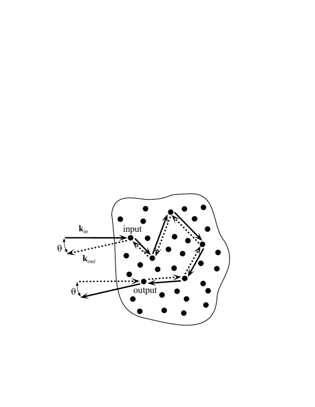
Figure 1: The origin of CBS.

If the scatterers’ respective positions are fixed, the light intensity scattered at angle $\theta$ results from the interference of many partially scattered waves and is a fast-varying function of $\theta$. This is the well-known speckle pattern (see fig 2A). Speckle is observed whether the medium is optically thin, with single scattering being dominant, or optically thick in the multiple scattering regime. Let us now imagine that a configuration averaging is performed : the respective positions of the scatterers in the sample are modified and the corresponding different speckle patterns are summed up, resulting in an averaged intensity distribution. In experiments, this is obtained either automatically due to the scatterer’s motion (e.g. in liquid samples), or by moving the sample so that different configurations are probed. As a result of this averaging process, we expect the speckle pattern to smooth out to give a relatively angle-independent intensity distribution. The main argument in this explanation is that the detected field is the coherent sum of scattered electric fields :

$$\mathbf{E}=\underset{j}{\sum}\mathbf{E}_{\text{j}}\exp\left(i\varphi_{\text{j}}\right)$$ (1)

The average detected intensity will then be :

$$\left\langle I\right\rangle=\left\langle\left|\underset{j}{\sum}\mathbf{E}_{\text{j}}\exp\left(i\varphi_{\text{j}}\right)\right|^{2}\right\rangle=\underset{j}{\sum}\left\langle\left|\mathbf{E}_{\text{j}}\right|^{2}\right\rangle+\underset{j\neq k}{\sum}\left\langle\mathbf{E}_{\text{j}}\cdot\mathbf{E}_{\text{k}}^{\ast}\exp\left(i\varphi_{\text{j}}-i\varphi_{\text{k}}\right)\right\rangle$$ (2)

where the brackets denote configuration averaging. A first approach would be to suppose that the phases $\varphi_{\text{j}}$ and $\varphi_{\text{k}}$ are uncorrelated random variables, which yields an interference term equal to zero :

$$\left\langle I\right\rangle=\left\langle\underset{j}{\sum}\left|\mathbf{E}_{\text{j}}\right|^{2}\right\rangle$$ (3)

However, this argument is wrong if the interference arises from two correlated fields. Such correlations can be very important in the case of spatial correlation of the scatterers, as e.g. for Bragg scattering in crystals. But even if there is no correlation in the position of the scatterers, the fields $\mathbf{E}_{\text{j}}$ and $\mathbf{E}_{\text{k}}^{\ast}$ can be correlated. In particular, this is the case for backscattering in the multiple scattering regime.

Indeed, let us consider for every scattering path (yielding some backscattering), the reverse path as represented on fig 1. This reverse path (dotted arrows) involves the same scattering sequence as the ”direct” path (solid arrows), but in inverse order. The geometrical phase difference between waves following these two paths is :

$$\Delta\varphi=\left(\mathbf{k}_{\text{in}}+\mathbf{k}_{\text{out}}\right)\cdot\left(\mathbf{r}_{\text{in}}-\mathbf{r}_{\text{out}}\right)$$ (4)

where $\mathbf{r}_{\text{in}}$ and $\mathbf{r}_{\text{out}}$ are the vector positions of  the first and last scatterers involved in the path (denoted by ”input” and ”output” in fig 1). One can thus see that if the relative position of the scatterers is randomly changing the phase difference is generally also a random parameter and the corresponding interference terms in eq.(2) will be cancelled. However, for the particular case of backscattering ($\mathbf{k}_{\text{in}}+\mathbf{k}_{\text{out}}=0$) this phase difference is always zero, regardless of the specific scattering path considered. Thus, the two waves following the reverse paths of fig 1 always add up constructively in the backscattering direction, and this interference survives the averaging process (this property is of course not verified for $\theta\neq 0$, where the interferences vanish). The remaining terms in eq.(2) arise from interference between distinct paths and are obviously zero since the fields are not correlated in this case. As a result, the averaged intensity distribution exhibits a peak centered at $\theta=0$, known as the CBS cone. This is illustrated on fig 2, where the intensity distributions for a given fixed configuration (A) and after configuration average (B) are recorded. Note that, in the case of a single configuration (speckle), one does not necessarily have a constructive interference in the backscattering direction.

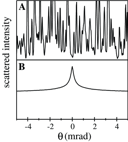
Figure 2: Interference effects and configuration average. A : backscattered intensity for one configuration of the sample (speckle) B : backscattered intensity after configuration average (CBS cone).

The ratio of the configuration-averaged scattered intensity at $\theta=0$ (exact backscattering) to the ”incoherent background” obtained at large angle is known as the CBS enhancement factor. If the amplitudes of the reverse paths, which interfere in the backscattering direction, are equal, the enhancement factor equals 2. However, this property is verified only if the single scattering light, which does not contribute to CBS, is removed from the detected signal. We will see in section 3.2 how this can be achieved by selecting the appropriate polarization channel.

2.2 Cone shape

The enhanced backscattering described above relies on the constructive interference between reverse paths. One can make an analogy with a Young’s interference experiment, where two diffracting slits would be positioned in place of the ”input” and ”output” scatterers (see fig 1). If the slits are backlit with a plane wave (of wave vector $-\mathbf{k}_{\text{in}}$), the interference produces a sinusoidal fringe pattern in the far field, with a maximum intensity at $\theta=0$ and a fringe spacing inversely proportional to the transverse spacing between the scatterers (this is valid only for small values of $\theta$). The total configuration-averaged intensity distribution is obtained by summing up incoherently the fringe patterns corresponding to all the possible scattering paths in the sample. This incoherent sum accounts for the fact that interferences between waves following distinct paths do not survive the configuration average. Since the fringe patterns all have a ”bright” fringe at $\theta=0$, the total intensity is maximum there, and decreases to an ”incoherent background” value within an angular range $\Delta\theta\sim\lambda/d$, where $d$ is the average transverse distance between slits (this is similar to the zero path-difference fringe observed in Michelson interferometers with white light). This analogy thus shows why the average light intensity is increased around the backscattering direction, and relates the angular width of the peak to the inverse of the distance between entering and exit points of the light in the sample.

More precisely, in the case of a semi-infinite medium and for scalar waves, the FWHM of the coherent backscattering cone is given by [8, 9] :

$$\Delta\theta_{CBS}\approx\frac{0.7}{kl^{\ast}}$$ (5)

where $k$ is the wave vector in the scattering medium, and $l^{\ast}$ is the transport mean free path. The transport mean free path describes the distance necessary, on average, for the initial direction of propagation to be scrambled (which is of course essential to observe backscattering). It is related to the scattering mean free path $l$ (mean distance between two scattering events) by:

$$l^{\ast}=\frac{l}{1-\left\langle\cos\theta\right\rangle}$$ (6)

where $\theta$ is the angle between the incident and scattered light (for a single scatterer), and the brackets denote the average over the radiation pattern of the scatterer. Thus, if $\left\langle\cos\theta\right\rangle=0$ the scattering and transport mean free paths are identical. Note that this condition does not imply that the radiation pattern is isotropic (think for instance of the dipole radiation pattern).

As it was evidenced with the Young’s slits analogy, the width of the coherent backscattering cone depends on the mean distance between the first and last scatterers. This distance will of course increase with the scattering order $N$ (number of scattering events) involved, so higher orders will yield narrower cones. For large scattering orders ($N\gg 1$) the propagation can be described as a random walk of step $l^{\ast}$, and the average distance between the input and output scatterers grows as $\sqrt{N}$ $l^{\ast}$ (diffusion approximation). In a semi-infinite medium where all scattering orders contribute, the total CBS cone is obtained by adding up the cones associated to each order. This implies to evaluate the weight $P(N)$ of each scattering order. Due to the presence of very high scattering orders (giving very narrow cones), the actual shape of the cone around the tip is triangular [10]. The resulting angular FWHM is given by eq.(5). The relationship between cone width and scattering order is illustrated on fig 3A, where are plotted the CBS cones associated to $N=2,3,10$ (thin lines) and the sum of all the contributions up to $N=80$ (bold line), in the case of a slab of non-absorbing medium of optical thickness $b=12$.

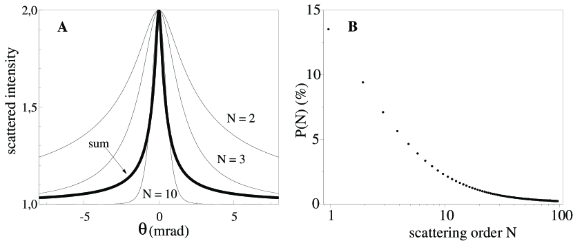
Figure 3: Contribution of different scattering orders in a slab of optical thickness $b=12$. A : CBS cones for $N=2,3,10$ and the sum of the first 80 orders B : contribution of each order to the backscattered intensity.

The scattered intensity is plotted as a function of the normalized backscattering angle $\theta kl^{\ast}$. These curves are obtained with a rigorous theory [11] for scalar waves, which does not rely on the diffusion approximation. Each cone is scaled by its own incoherent background for better comparison of the widths, so the respective amplitudes of the different orders do not appear on this plot. It can be seen that the width of the cone decreases as the scattering order increases (the double scattering cone is approximately 10 times broader than the ”total” peak). The shape is also clearly affected, for instance in the ”wings” of the cones ($\theta kl^{\ast}\gg 1$) : for $N=2$, the scattered intensity decreases as $1/\theta$ while the sum of all the other contributions decreases as $1/\theta^{2}$ [12]. On B are plotted the weights $P(N)$ corresponding to each scattering order. Asymptotically, the weight of the $N^{th}$ order decreases as $N^{-3/2}$ [11].

Thus, we emphasize that the CBS cone shape is in general determined not only by the transport mean-free path, as in the case of a semi-infinite medium (eq.(5)), but also by the sample geometry through a truncation of the scattering orders. A similar effect is obtained in the case of an absorbing medium, where the contribution of long light paths is reduced.

3 Experiments with classical scatterers

We now turn to the description of CBS experiments using classical samples such as milk, suspensions of TiO₂ particles, or teflon. We discuss several effects that can affect the CBS signal.

3.1 Description of the experimental setup

The CBS detection setup used in our experiment is schematically represented on fig 4. The sample is illuminated by a collimated laser probe ($1/e^{2}$ waist 7,6 mm). Most of the backscattered light ($\sim$90%) is reflected by a beam-splitter, and its angular (far field) distribution is recorded on a cooled CCD placed in the focal plane of an analysis lens ($f=190$ mm). Since the focussing is quite critical, the CCD camera is mounted on a translation stage. By rotating the polarizer and quarter-wave plate, one can select the polarization channel where the signal is detected (see section $3.1.3$).

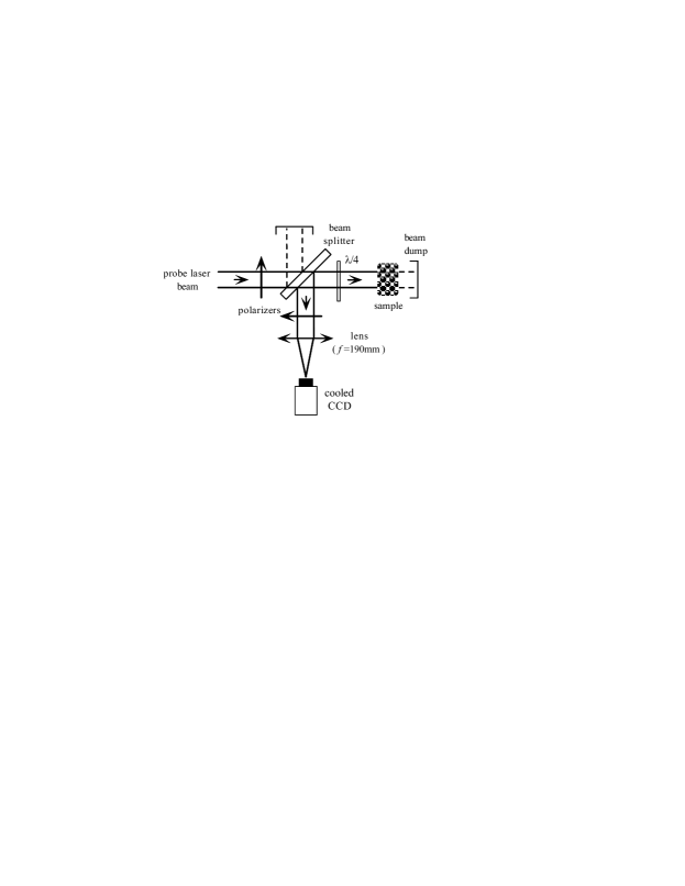
Figure 4: CBS detection setup.

As usual in CBS experiments, great care must be taken to shield the detector against stray light; the alternative paths that can be followed by the light (incident beam reflected by the beam-splitter and beam transmitted by the sample) must also be carefully blocked to avoid any unwanted backscattering. This is achieved by inserting a neutral filter at Brewster angle in the unwanted beam paths. The residual reflection by the neutral filter is directed onto a black paper.

Another possible source of stray light originates from reflections inside the beamsplitter. This is avoided by using a beamsplitter with a small wedge ($5{{}^{\circ}}$). This beamsplitter has different reflection coefficients for s- and p-polarized light (polarization orthogonal or parallel to the plane of incidence respectively), which have to be accounted for when comparing data in different polarization channels. Another consideration is the angular response of the detection optics (quarter-wave plate + beam-splitter + polarizer), which should be sufficiently flat within the angular field of observation to avoid deformation of the background level. However, because of our small detection angular range ($\simeq 15$ mrad), this effect is negligible in our case.

The use of a cooled CCD with low thermal (and readout) noise allows for long integration times yielding improved signal-to-noise ratio. This is also convenient to record CBS cones from self-averaging samples such as milk or a suspension of TiO₂ particles, where the CCD camera integrates the scattered light for several tens of ms up to several minutes, depending on the time scale of the motion of the scatterers.

3.1.1 Angular resolution

To detect CBS cones with a small angular width, it is important to avoid convolution due to the residual divergence of the incident laser beam and to aberrations of the detection optics. The probe beam collimation is achieved using a telescope including a spatial filter, and shear plate interferometry [13] as a diagnostic technique. The diffraction limit corresponding to our beam waist size is $\Delta\theta_{\text{diff}}\simeq 0.03$ mrad FWHM, below the resolution limit due to the CCD’s pixel size $\Delta\theta_{\text{pix}}\simeq 0.05$ mrad. For technical reasons linked to the experiment with cold atoms, the actual detection optics is more complicated than represented on fig 4 and includes an image transport system between the focal plane of the analysis lens and the CCD (see fig 12). All the lenses in the detection system are achromatic doublets to minimize aberrations.

The most direct way to estimate the effective angular resolution of the experimental setup is to record the CBS cone from a liquid sample, milk for instance, which is gradually diluted to increase the scattering mean free path (thus reducing the width of the cone). Once the cone becomes narrower than the angular transfer function of the apparatus, the observed signal is strongly reduced due to convolution and its width is essentially that of the transfer function. Using this procedure, we find an effective angular resolution $\Delta\theta_{\text{res}}\simeq 0.1$ mrad. We believe this value results from residual aberrations in the optical system. Knowing the effective resolution, it is then possible to compute the broadening and reduction of the CBS cone due to convolution.

Although it has many advantages, the choice of a CCD also implies that the angular dynamics of our detection is somewhat limited (the CCD has $770\times 512$ pixels) compared to, for instance, the system of ref[14]. Because of the far-reaching wings of typical CBS cones, it is difficult to have at the same time an angular magnification (determined by the focal length of the analysis lens) good enough to look at the shape of the cone around the tip, and an angular field wide enough to see the wings.

3.1.2 Signal acquisition and treatment

Here we describe our standard procedure to obtain a CBS cone profile such as that shown on fig 14. First an image of the CBS cone is recorded. The configuration average is performed using a small rotor (solid samples) or simply by the motion of the scatterers (liquids, cold atoms). A typical integration time is 20 s. Then, a second ”background” exposure is taken without sample, and subtracted from the signal to remove residual stray light. This step will be discussed in more details in the case of an atomic sample.

Once the image is obtained, a cross-section is taken to obtain a profile. However, in the case of a noisy signal, we perform an angular average on the CCD image to smoothen the CBS profile : the center of the CBS peak is pinpointed, and a number of different cross-sections passing through this center are averaged to give the final signal. We emphasize that this technique can only be employed if the cone is isotropic, which is the case only in certain polarization channels (see section $4.3.3$). We checked that, in the appropriate channels, this procedure yields the same profile as when using a simple cross-section.

The remaining problem is the determination of the enhancement factor, which implies an estimation of the level of the incoherent background. As already mentioned, the wings of the cone are quite wide and a direct measurement of this background level is difficult. Thus, we fit the experimental profile with a sum of four lorentzian curves, all centered on $\theta=0$ but with widths and heights as free parameters. The value of the background is also returned by the fit and used to determine the enhancement factor. This empirical approach allows to fit, using the same procedure, different cone shapes whose analytical expressions are not known. To estimate its accuracy, we applied the technique to two different theoretical cone shapes : a cone from a semi-infinite medium (diffusion theory, $I\left(\theta\right)\varpropto 1/\theta^{2}$ for $\theta\ \gg\lambda/l^{\ast}$) and a double-scattering cone ($I\left(\theta\right)\varpropto 1/\theta$ for $\theta\gg\lambda/l^{\ast}$). For an angular field of detection about 20 times wider than the FWHM of the cones (typical experimental situation), the error on the enhancement factor is below 1%. The actual uncertainty on the enhancement factor originates from the fact that our smoothing procedure does not improve the signal-to-noise ratio at the cone tip, because this particular point is common to all the profiles averaged. To reduce the uncertainty, we average the signal from a few neighboring pixels around the center of the cone, but the improvement is limited since the corresponding angular range must remain smaller than the resolution. We finally estimate the uncertainty on the enhancement factor $f_{e}$ to be around $f_{e}\pm 0.01$.

3.2 Polarization effects

An important aspect of all coherent backscattering experiments with light is the vector nature of the scattered wave, i.e. the polarization of the light. Thus, controlling the incident and detected polarizations is essential in these experiments.

For a linear incident polarization (quarter-wave plate removed), we record (by rotating the detection polarizer) the scattered light either with linear polarization parallel (”parallel” channel  or $lin$ $//$ $lin$) or orthogonal (”orthogonal” channel or $lin\perp lin$) to the incident one. We also use a circular incident polarization by inserting the quarter-wave plate between the beam-splitter and the sample. In the ”helicity preserving” channel (denoted $h$ $//$ $h$) the detected polarization is circular with the same helicity (sign of rotation of the electric field referenced to the direction of wave propagation) as the incident one : in this channel, no light is detected in the case of the back-reflection from a mirror. The ”orthogonal helicity” channel ($h\perp h$) is obtained for a detected circular polarization orthogonal to the previous one. When defining the polarization by referring to a fixed axis (as one usually does in the atomic physics community), an incident $\sigma^{+}$ light would remain $\sigma^{+}$ by reflection from a mirror. The $h\perp h$ channel is thus a $\sigma^{+}/\sigma^{+}$ channel, and the $h$ $//$ $h$ channel corresponds to a polarization flip from $\sigma^{+}$ to $\sigma^{-}$.

The choice of the appropriate polarization channel makes it possible, at least for some categories of scatterers, to remove the single scattering contribution to the detected light. Indeed, single scattering does not contribute to CBS but adds up to the signal as a background, and thus reduces the apparent enhancement factor (defined as the ratio of the detected intensities at $\theta=0$ and $\theta\gg\lambda/l^{\ast}$). In the case of single (back)scattering, ”spherical” scatterers e.g. Rayleigh (size $a<\lambda$) and spherical Mie ($a\gtrsim\lambda$) scatterers behave like mirrors : they flip the helicity of circularly-polarized light. Thus, CBS experiments are usually performed in the $h$ $//$ $h$ channel where the single scattering contribution is rejected. Furthermore, the reciprocity principle [15] can be used in this channel, and predicts an enhancement factor of 2. In the case e.g. of non-spherical scatterers, the single scattering contribution is present even in the $h$ $//$ $h$ channel and the expected enhancement factor is smaller than 2 [16].

Polarization can also affect the enhancement factor through more subtle ways. This is illustrated on fig 5 with the example of $N=3$ scattering and dipole scatterers.

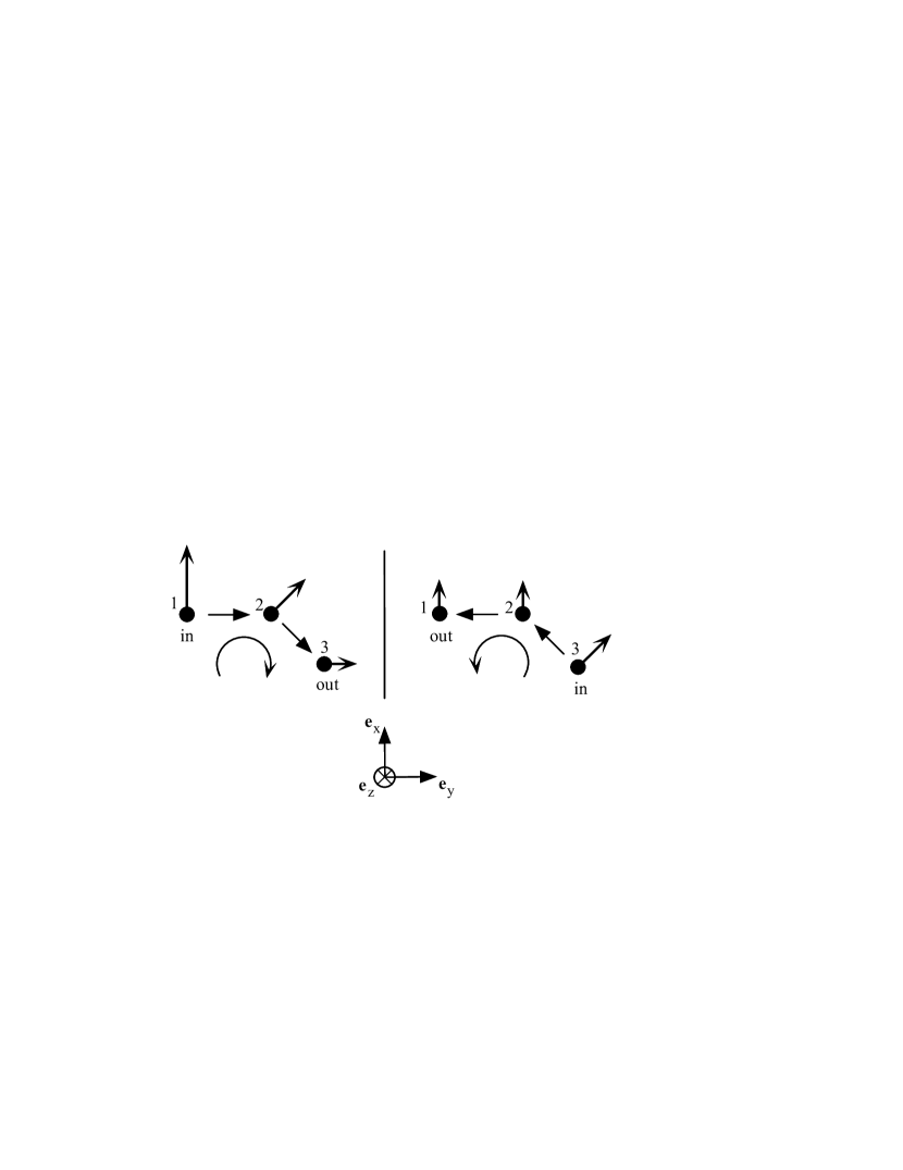
Figure 5: Reduction of enhancement factor in the $lin\perp lin$ channel.

The incident wave vector is orthogonal to the plane of the figure (parallel to $\mathbf{e}_{\text{z}}$), where all the scattering events are supposed to take place. We consider the case of detection in the $lin\perp lin$ channel : the incident wave polarization is parallel to $\mathbf{e}_{\text{x}}$ and the detected polarization along $\mathbf{e}_{\text{y}}$. The arrows mark the polarization of the wave after each scattering. This figure illustrates the fact that the amplitudes of the reverse paths that interfere to give rise to the cone are different in this channel : for the path on the left (scattering sequence $1\rightarrow 2\rightarrow 3$) some light comes out in the polarization orthogonal to the incident, while for the reverse sequence ($3\rightarrow 2\rightarrow 1$) the projection on the detected polarization is zero. Since the amplitudes of the two waves are imbalanced, the contrast of the interference will be reduced and hence the CBS enhancement factor. This contrast reduction effect becomes more effective as the order of scattering $N$ increases. Thus, in the case of  ”spherical” scatterers, the enhancement factor in the ”orthogonal” channels (linear and circular) is 2 for $N=2$ [9], and decreases fast for higher orders. For aspherical scatterers (e.g. antennas), the enhancement factor in the orthogonal channels is smaller than 2 even for $N=2$.

When multiple scattering occurs, the polarization of the incident wave is rapidly scrambled. This phenomenon is illustrated on fig 6.

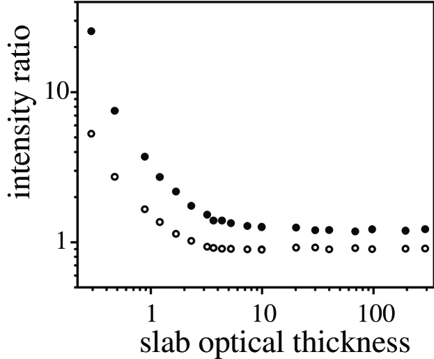
Figure 6: Depolarization due to multiple scattering.

On this plot we reported the ratio of the intensities scattered in crossed channels for an incident circular polarization (ratio $=I_{h//h}/I_{h\perp h}$, open circles) and linear polarization (ratio $=I_{lin\perp lin}/I_{lin//lin}$, full circles), as a function of the optical thickness of the sample. The sample is a solution of TiO₂ particles (size $\simeq$ $200$ nm) in a cell with a slab geometry (thickness 7 mm). The concentration of the solution is gradually varied to modify the optical thickness of the slab. At low optical thickness, single scattering is dominant and the sample behaves like a ”diffusive mirror” : the polarization remains almost unaffected and the scattered light is detected mainly in the $lin$ $//$ $lin$ channel for incident linear light, and in the $h\perp h$ channel for circular light. As optical thickness is increased, higher orders of scattering appear and an increasing amount of light is redistributed in the orthogonal channels. For high values of the optical thickness, the light is almost depolarized and the intensity ratio is close to unity. The fact that the curve for linear polarization is above that for circular light is probably due to the contribution of low scattering orders (which is significant even in a semi-infinite medium[11]). Indeed, it is known that the ”memory” of the initial polarization is preserved longer for linear than for circular polarization in the case of Rayleigh scatterers [17].

3.3 Enhancement factor

The accurate determination of the enhancement factor in CBS experiments is quite delicate [10]. Indeed, the observed enhancement factor is usually quite smaller than the theoretical prediction of 2. This reduction may arise from many causes. We have already mentioned the convolution due to the experimental resolution and the divergence of the probe beam. We also saw, in the previous section, that the theoretical enhancement factor is smaller than 2 in the $lin\perp lin$ and $h\perp h$ channels. Reciprocity predicts an enhancement factor of 2 in both the $lin$ $//$ $lin$ and $h$ $//$ $h$ channels. This is assuming that single scattering is eliminated, which is possible only in the $h$ $//$ $h$ channel (for spherical or Rayleigh scatterers). Thus, in channels other than $h$ $//$ $h$, the enhancement factor depends a priori on the sample geometry and optical thickness.

However, even in the $h$ $//$ $h$ channel, another effect can reduce the enhancement factor. As emphasized by the Young slits analogy, CBS is essentially a two-waves interference effect. What determines the contrast of the interference is the correlation between the fields at the input and output scatterer positions. This correlation includes both differences in amplitude and phase of the waves at the two points. For instance, the intensity distribution can be homogeneous and the phase vary in the transverse plane : in this situation of partial spatial coherence, the enhancement factor is decreased [18][19]. In the case of a gaussian laser beam, the spatial coherence is high and it is rather the inhomogeneous intensity profile that plays a dominant role, as shown on fig 7. If the distance between the first and last scattering event of a given path is larger than the transverse size of the laser beam $w$, then the amplitudes of the direct and reverse path are imbalanced and the enhancement factor will be reduced. One expect the reduction effect to be more important for increasing values of $l^{\ast}/w$. In most samples $l^{\ast}\ll w$ and this effect remains small. However, we will see in section $4.3.1$ that in the case of the atomic sample the above condition is not necessarily fulfilled, and this reduction effect should be considered.

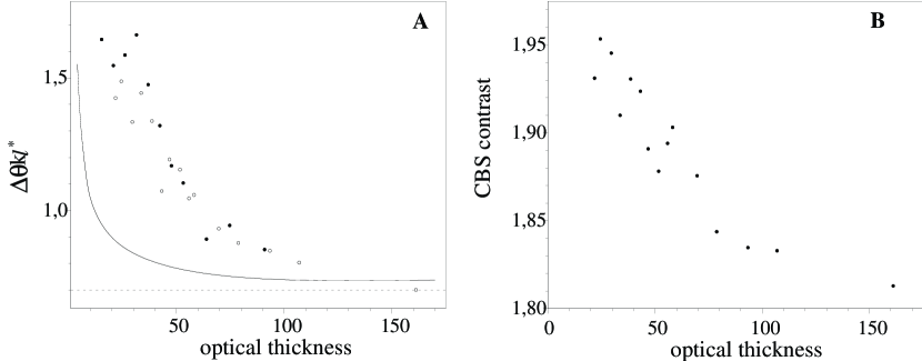
Figure 7: Effect of intensity profile on the enhancement factor.

3.4 Role of sample geometry

In the case of a semi-infinite medium, the CBS cone width gives direct access to the transport mean free path $l^{\ast}$ trough eq.(5). However, in the case of a finite medium, this simple relationship does not hold anymore, due to the truncation of long light paths. This yields a higher relative contribution of low scattering orders and hence a broader cone. How strong this broadening is depends on the actual geometry of the sample. For instance, in a spherical sample of diameter $\phi$, high scattering orders will be truncated faster than in a slab of thickness $e=\phi$.

To illustrate the importance of sample geometry, we have reported on fig 8 the results from CBS experiments on spherical samples of polystyrene foam with different diameters.

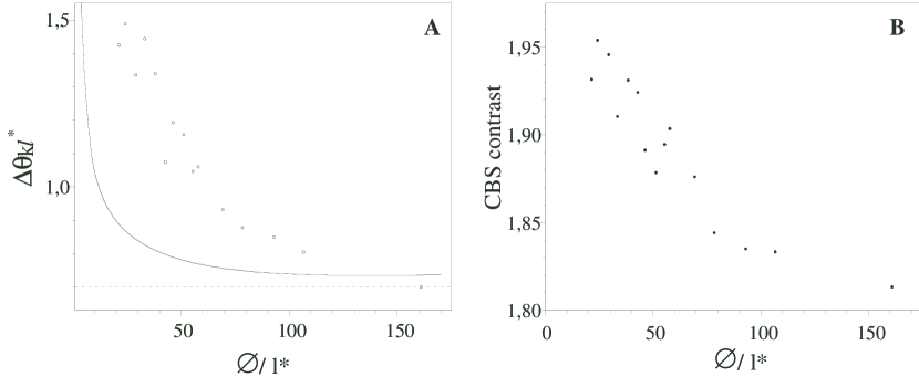
Figure 8: CBS experiments on spherical polystyrene samples. A : measured cone width as a function of $\phi/l^{\ast}$ (circles), and theoretical cone width for a slab of thickness $\phi$ (line) B : measured CBS enhancement factor as a function of $\phi/l^{\ast}$.

In fig 8A we plotted the product $\Delta\theta_{CBS}kl^{\ast}$ (where $\Delta\theta_{CBS}$ is the cone’s angular FWHM) as a function of the ”optical diameter” defined as $\phi/l^{\ast}$, where $\phi$ is the diameter of the sample. The value of $l^{\ast}\approx 0.18$ mm was deduced from the width of cones from bulk samples using eq.(5). The circles correspond to the experiment. The solid line is the prediction of a rigorous theory [11] for scalar waves and a slab geometry ; the horizontal axis thus correspond , for this curve, to the optical thickness $b=e/l$ where $e$ is the slab thickness (we assume $l=l^{\ast}$). One can see that the CBS cone from a spherical sample starts to broaden even at large $\phi/l^{\ast}$ ratio, which reflects the fact that long light paths are truncated faster than in the slab geometry. We will see that in the case of the atomic sample, the symmetry is spherical but with a non uniform (quasi-gaussian) density profile; we thus can expect truncation effects to play an important role in this situation. In B is reported the measured enhancement factor, which increases significantly as the sphere’s diameter decreases (the peak’s height increases by $\sim 15\%$). Two effects tend to increase the enhancement factor. Due to the truncation of long scattering paths, the cone is broadening and the convolution by the transfer function of the apparatus is decreased. However, this does not seem enough to fully explain the observed increase in enhancement factor. We think that part of this improvement is due to an increasingly uniform illumination of the sample, reducing the imbalance effect of fig 7.

3.5 CBS with ”single scattering”

We mentioned in section $3.2$ that single scattering does not contribute to the CBS signal. However, there is a situation where average-robust interference effects can be observed with single scattering : the case of an optically thin sample in front of a mirror. This situation is depicted on fig. 9.

Figure 9: CBS with “single scattering” : principle.

The scattering medium being optically thin, a certain amount of light reaches the mirror and is reflected. The mirror plays the role of a second scatterer with a very anisotropic radiation pattern due to specular reflection. Fig. 9A and B illustrate two processes that yield a constructive interference after configuration average. Process A corresponds to the ”usual” backscattering situation, while the example B shows that the interference is also constructive at an angle $2\alpha$ from the incident direction. In the far field, this gives a ”ring” of angular diameter $2\alpha$ for the enhanced scattered intensity, centered on the direction of the normal to the mirror. The effect can also be understood as double scattering by the ”real” scatterer and its image in the mirror.

This ”single-scattering cone” can be observed when one performs CBS experiments on dilute liquid samples in a glass cell of slab geometry. The 4% reflection from the back of the cell is enough to yield an important contrast of the interference, as illustrated on fig. 10 A and B.

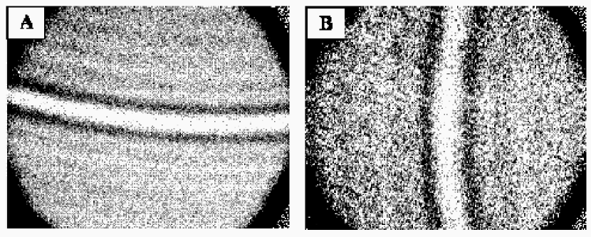
Figure 10: CBS with ”single scattering” : experiment. A : Mirror tilted vertically B : mirror tilted horizontally.

In this experiment, a dilute solution of TiO₂ particles was placed in a quadrangular glass cell of thickness 7 mm. The optical thickness of the slab was $b=0.6$. This is not a pure single scattering situation, but higher scattering orders are not dominant. The images were recorded in the $lin$ $//$ $lin$ channel, with an incident polarization vertical in the plane of the figure. In fig. 10 A the cell was tilted vertically so that the vector normal to the back face points upwards. The image shows the section of the enhanced intensity ring in a narrow angular range around the backscattering direction, which is almost an horizontal line. When the cell is tilted horizontally, we obtain the vertical line of fig. 10 B. To confirm that the effect arises from scattering, we replaced the solution in the cell by pure water, and the ring disappeared. Since the process involves only single scattering (and the reflection from a mirror), the polarization is preserved around the backscattering direction. Thus, when we recorded the backscattered intensity in the $lin\perp lin$ channel, the ring also disappeared.

It is thus possible with this configuration to study an interference effect very similar to CBS, but in the single scattering regime. This is an interesting possibility in the case of an atomic sample, as the theory becomes much simpler.

4 Experiments with cold atoms

4.1 Properties of atomic scatterers

Coherent backscattering constitutes a new tool to probe the properties of cold atoms. Indeed, atoms as elementary scatterers are an interesting medium to study the quantum manifestations of the interaction between light and matter. As a consequence of the discrete energy levels, the atom’s scattering cross-section is highly resonant (Q $\approx 10^{8}$) and the resonance frequency is identical for all the scatterers in the sample (assuming a negligible Doppler effect, which implies laser cooling). Such a situation would be very difficult to achieve with classical resonators like, for instance, dielectric spheres of high finesse. Due to this narrow resonance, the light mean free path in the atomic medium can be varied by orders of magnitude by shifting the wave frequency a few linewidths away from the atomic transition. As we will see in section $4.3.1$, the presence of an internal structure in the ground state (Zeeman sublevels) has some other profound consequences on the CBS signal from the atomic sample used in our experiment.

Several reasons motivate the use of cold atoms to observe CBS. Firstly, Doppler broadening is then reduced and all the atoms have the same resonant scattering cross-section, characterized by the natural width $\Gamma$ of the atomic transition ($\Gamma/2\pi\approx$ 6 MHz for rubidium). However, the atom’s motion has a more important consequence on CBS : if the motion of the scatterers is fast compared to the time for the scattered wave to pass through the medium, the two reverse waves of fig 1 will encounter different configurations, resulting in a ”dynamic” break down of reciprocity. For non resonant scatterers, the typical time scale to consider is the propagation time between two scattering events, so this effect requires extremely fast (almost relativistic) motion [20]. In the case of quasi-resonant scattering by atoms, however, the time scale is considerably increased by the large delay time $\tau=\partial\varphi/\partial\omega$ [21], where $\varphi$ is the scattered wave phase-shift and $\omega$ the angular frequency. Taking as a criterion for the break down of the coherent backscattering cone that each scatterer has moved by one wavelength during that typical time scale :

$$\Delta x=v\tau\gtrsim\lambda$$ (7)

and taking an on-resonant scattering dwell time $\tau_{res}=2/\Gamma$, one requires to observe CBS velocities smaller than :

$$v_{crit}\backsim\frac{\lambda}{\tau_{res}}=\frac{\lambda\Gamma}{2}$$ (8)

In terms of Doppler broadening, this corresponds to :

$$kv_{crit}\backsim\Gamma$$ (9)

The above criterion shows that if one employs resonant laser light on a dilute atomic gas (to maximize the optical thickness of the sample and favor multiple scattering), one has first to laser-cool these atoms in order to observe CBS. For rubidium atoms, satisfying condition (9) implies cooling down the atomic sample below $T_{crit}=0.25K$, a regime easily reached by standard techniques. However, in the case of higher orders of scattering, the dwell time has to be multiplied by the number of scattering events and the above criterion imposes lower temperatures.

One could however consider the possibility of using atomic gases at room temperature. But, in order to fulfill (8), one would have to detune the laser frequency from resonance in order to lower the dwell time. This would yield the condition :

$$\tau=\frac{2}{\Gamma}\frac{\left(\Gamma^{2}\diagup 4\right)}{\delta^{2}+\left(\Gamma^{2}\diagup 4\right)}\lesssim\frac{\lambda}{v}$$ (10)

or

$$\left(\frac{\delta}{\Gamma}\right)^{2}\gtrsim\frac{kv}{\Gamma}$$ (11)

On the other hand, increasing the detuning will decrease the scattering cross-section and hence the optical thickness $b\left(\delta\right)=n\sigma\left(\delta\right)L$ of the sample (where $n$ is the atomic density, $\sigma$ the scattering cross-section and $L$ the thickness of the sample). To obtain an optical thickness larger than unity, one has to fulfill :

$$b\left(\delta\right)=b\left(0\right)\frac{\left(\Gamma^{2}\diagup 4\right)}{\delta^{2}+\left(\Gamma^{2}\diagup 4\right)}\gtrsim 1$$ (12)

or

$$\left(\frac{\delta}{\Gamma}\right)^{2}\lesssim b\left(0\right)$$ (13)

The two conditions 11 and 13 can be fulfilled simultaneously if :

$$b\left(0\right)\gtrsim\frac{kv}{\Gamma}$$ (14)

i.e. if the on-resonance optical thickness $b\left(0\right)$ of the medium is larger than the Doppler broadening in units of $\Gamma$. It seems to be possible to be realize such situations in hot atomic vapors, but up to now no coherent backscattering of light by hot atoms has been reported.

4.2 Preparation of the atomic sample

The first step in our experiment is to prepare an atomic sample dense enough to reach the multiple scattering regime. The relevant parameter is the optical thickness of the atomic cloud $b$. To study multiple scattering of light in the atomic medium, one needs typically $b>1$.

A magneto-optical trap (MOT) is loaded from a room-temperature vapor of rubidium atoms in a quartz cell, as shown on fig. 11.

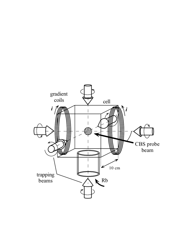
Figure 11: Setup of the magneto-optical trap.

The atoms are trapped by six independent laser beams : this configuration (instead of the usual three retro-reflected beams) allows to avoid the imbalance in trapping beams intensity due to the high optical thickness, and thus to obtain stable trapping. The beams parameters are : wavelength $\lambda=780$ nm (D2 line of rubidium), detuning from resonance $\delta\approx-3\Gamma$, diameter 2.8 cm (FWHM) and power per beam 30 mW. The large beam size increases the number of trapped atoms, but requires more laser power. These trapping beams are obtained by splitting a single 200 mW beam, produced by single-pass amplification of a 4 mW beam through a tapered amplifier (SDL TC30-E). The source laser diode is injection-locked to a reference DBR laser diode (Yokogawa YL78XNW/S). A magnetic field gradient of typically 10 G/cm is applied to spatially confine the cold atoms. The CBS laser probe lies in the horizontal plane of the figure, at an angle of approximately 25^∘ from the trapping beam.

To characterize the trap, we record the fluorescence on a photodiode and a CCD ; we also measure the transmission of a the CBS laser probe through the atomic cloud to determine its optical thickness. The data from these two methods are in good agreement. The temperature of the cloud is measured by time-of-flight. The MOT contains approximately $10^{9}$atoms with a quasi-gaussian spatial distribution of width typically 7 mm FWHM. The MOT loading time is typically of $0.6\sec$. Transmission measurements using the $3\rightarrow 4$ transition of the D2 line yield a typical optical thickness b $\simeq$ 3. The rms velocity of the atoms is 10 cm/s, small enough to fulfill the criterion discussed above.

To observe the CBS cone, we have to turn off the MOT trapping beams. This is because the fluorescence of the atoms excited by the trapping lasers (total scattered power $\simeq$ 4 mW!) is much brighter than the light scattered from the probe. Also, it seems preferable to avoid perturbations of the atoms by the trapping lasers during the CBS measurement. Thus, we alternate a ”MOT phase” (duration 20 ms) where the atoms are trapped, with a ”CBS” phase (2-3 ms) where the trapping beams, repumper and magnetic field are switched off (switch-off time $<$0,2 ms) and the CBS signal recorded ; this phase is sufficiently short so that all the atoms remain in the capture zone and are efficiently recaptured when the MOT is switched back on. In fact, what limits the duration of the CBS phase is the maximum number of photons that can be scattered by each atom before it is ”pushed” out of resonance due to momentum transfer or pumped to the F $=2$ hyperfine level. For our rubidium atoms, this requires around 1000 photons, which are scattered within 5ms for a saturation parameter $s_{0}=0.01$. With the ”duty cycle” described above, the number of atoms in the trap is stationary and we can chain many such cycles. One problem is that the CCD camera which detects CBS can not be triggered at such a high rate. The CCD remains all the time in the ”acquisition” mode and thus has to be protected from the bright light scattered during the MOT phase. This is achieved using a chopper wheel as shown on fig. 12.

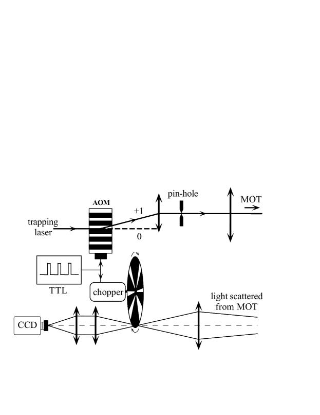
Figure 12: Synchronization of the detection.

The chopper is placed in the focal plane of the analysis lens. A transport system images this focal plane on the CCD. The trapping laser is turn on an off with an acousto-optic modulator (residual power 0.2 $\mu$W per beam). The same TTL signal is used to drive the modulator and as a reference for the controller of the chopper. The phase is adjusted so that the chopper blades block the detection path when the trapping laser is on. With this system, we are able to take exposures up to several tens of minutes. A typical total exposure time is 1 minute, with a detected flux of photons between 140 and 1400 photons/pixel/s.

It is necessary to acquire a ”background” image without cold atoms to subtract stray light. However, this procedure is more critical than in the case of classical samples, because this stray light originates from different sources. For instance, one could take the background exposure with no magnetic field gradient applied during the MOT phase, which prevents the trapping. However, in this case, a molasse is still operating during the MOT phase that produces a sample of cold atoms (with density increase in velocity-space). To avoid this, one need to turn off either the repumper or the trapping beams to take the background exposure. In this situation, the background signal originates essentially from scattering of the probe beam by hot atoms in the cell.

4.3 Results

4.3.1
Discussion of the atomic CBS signal

Fig. 13 shows the profiles of the atomic CBS cones in the four polarization channels (after angular average).

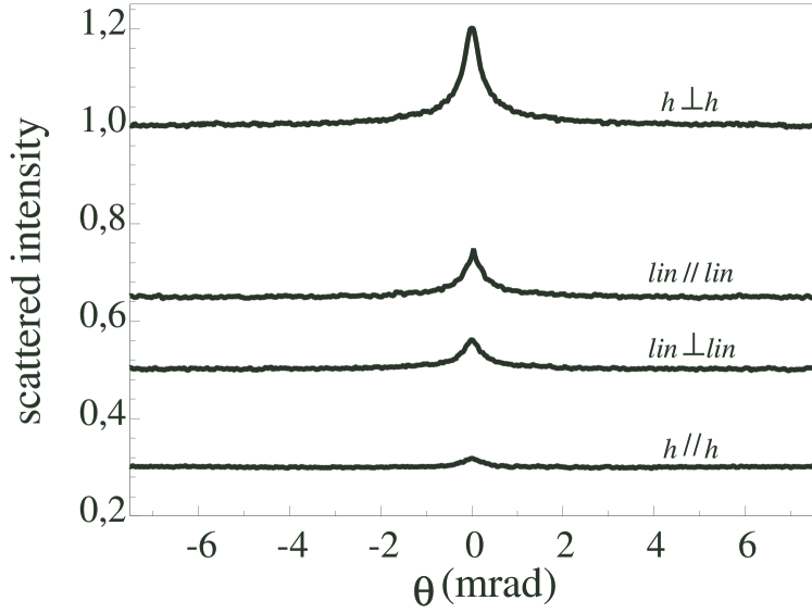
Figure 13: Atomic CBS profiles in the four polarization channels.

The detected intensity has been scaled so that the incoherent background of the $h\perp h$ curve is equal to unity. In this experiment, the on-resonance optical thickness measured through the center of the trap is $b=3$ for a quasi-gaussian cloud profile of diameter $\phi\simeq 4.8$ mm FWHM, yielding a peak density of $4\times 10^{9}$ cm^-3 and a scattering mean-free path $l\simeq 1.7$ mm at the center of the trap. A low-intensity probe beam was used, yielding a saturation parameter $s_{0}=0.01$. The total exposure (including the ”dark” periods) lasted 160 s.

The values of the enhancement factor are $1.20$ ($h\perp h$), $1.06$ ($h$ $//$ $h$), $1.15$ ($lin$ $//$ $lin$) and $1.12$ ($lin\perp lin$) respectively. The cone width, roughly independent of the polarization, is about $0.5$ mrad FWHM. We thus observe that the enhancement factor is much smaller than 2 in all polarization channels. Even more striking, the enhancement is only 1.06 in the $h$ $//$ $h$ channel, where reciprocity predicts a value of 2 for classical (and spherical) scatterers. It is clear that this reduction can not be attributed to the angular resolution of the apparatus. For a cone width of 0.5 mrad, we expect a reduction of the enhancement by 5% at most. This is confirmed by the observation of a CBS cone from a sphere of polystyrene, which has about the same width as the atomic cone (fig. 14). The enhancement factor is here of 1.96.

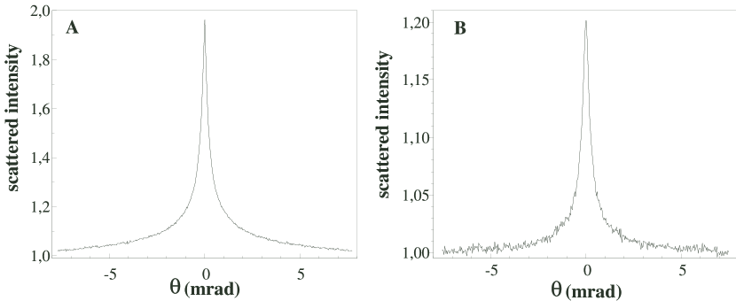
Figure 14: CBS cones from A : a sphere of polystyrene foam ($h$ $//$ $h$) B : the atomic cloud ($h\perp h$).

The explanation of this phenomenon lies in the atom’s internal structure of the ground state. First, because our atom is not a two-level system (or a $0\rightarrow 1$ transition), it has a non-negligible probability to make ”spontaneous Raman” transitions. In such a scattering event, the atom’s internal state (here the Zeeman sublevel of the ground state) after the scattering is different from the initial state, and the polarization of the scattered light differs from the incident one. Thus, for most transitions, the single scattering contribution can not be rejected even in the $h$ $//$ $h$ channel. In this respect, atoms behave similarly to strongly non-spherical classical scatterers (like e.g. oblate dielectric spheroids).

A more subtle effect is an imbalance between the amplitudes of the reverse paths that interfere to give the CBS cone. This is illustrated by the simple example on fig. 15 : we consider double scattering by atoms with a $1/2\rightarrow 1/2$ transition, in the $h$ $//$ $h$ channel. The quantification axis is taken along the wave vector of the incident laser light (parallel to $\mathbf{e}_{\text{z}}$). The incident light is polarized e.g. $\sigma^{+}$ and only the $\sigma^{-}$ component of the scattered light is detected in the $h$ $//$ $h$ channel.

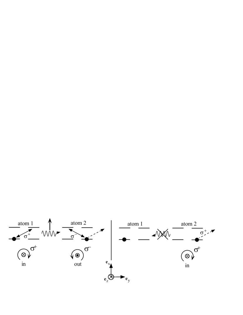
Figure 15: Imbalance effect due to the atom’s internal structure.

We suppose that the two atoms are in different Zeeman sublevels. We only consider the case of Rayleigh scattering (no change of Zeeman sublevel). In the first path (sequence $1\rightarrow 2$, left), atom 1 makes a $\sigma^{+}$ transition and radiates some light toward atom 2 with a linear polarization parallel to $\mathbf{e}_{\text{x}}$. This is seen by atom 2 as a superposition of $\sigma^{+}$ and $\sigma^{-}$ light ; since a $\sigma^{+}$ transition is not available, only $\sigma^{-}$ light is backscattered and detected in the $h$ $//$ $h$ channel. In the reverse path (right), there is no possibility for atom 2 to make a $\sigma^{+}$ transition : the amplitude of this path is zero. This is of course an extreme situation, but calculations[22] indicate that this effect reduces strongly the enhancement in the various channels. These calculations assume double-scattering in a semi-infinite medium, low saturation, a uniform distribution in the ground state Zeeman sublevels, and do not include optical pumping effects. Both Rayleigh and Raman transitions are included, the later also contributing to CBS. A detailed presentation of these calculations will be reported elsewhere[22]. The results for a $3\rightarrow 4$ transition are summarized below :

$$h$$

This table contains the contributions to the bistatic coefficient [23] of the ”crossed” (or interference) term $\gamma_{c}$, ”ladder” (or incoherent) term $\gamma_{l}$, and single scattering term $\gamma_{s}$ at exact backscattering ($\theta=0$). The effective enhancement factor in the presence of single scattering is then :

$$enhancement=\frac{\gamma_{c}+\gamma_{l}+\gamma_{s}}{\gamma_{l}+\gamma_{s}}=1+\frac{\gamma_{c}}{\gamma_{l}+\gamma_{s}}$$ (15)

Even though the model considers only double scattering and a semi-infinite medium, the values of  the table above are surprisingly close to the experimental observations. They reproduce the order of magnitude of the enhancement factor and even the hierarchy between the different channels (for instance, the enhancement is predicted to be smallest in the $h$ $//$ $h$ channel). Note that the reduction of the CBS enhancement factor has different origins in different channels : in the $h$ $//$ $h$ channel, most of the reduction stems from the imbalance mechanism of fig 15 ($1+\gamma_{c}/\gamma_{l}=1.214$), while a strong single scattering contribution explains most of the enhancement reduction in the $h\perp h$ channel.

The angular width of the atomic cone is $\Delta\theta_{CBS}\approx 0.5$ mrad. This value is about 10 times larger than what is obtained with eq.(5) and the estimated mean-free path of $1.7$ mm at the center of the trap. This is not surprising, since our sample is very far from a semi-infinite medium. Because of the spherical symmetry, gaussian density and rather modest optical thickness of the cloud, low orders of scattering are expected to dominate, yielding a broader cone. A Monte Carlo simulation is being developed to quantitatively address the problem of our particular sample geometry.

4.3.2 Effect of cloud density

By varying the trap parameters e.g. the magnetic field gradient (during the MOT phase), we can modify to a certain extent the characteristics of the atomic cloud (size and density). This modifies the width of the CBS cone, as shown on fig. 16A.

Figure 16: Effect of atomic cloud density on the CBS signal ($h\perp h$). A : cone width as a function of the optical thickness at the center of the cloud B : enhancement factor.

In this experiment, the value of the magnetic field gradient applied during the MOT phase was varied; this acts on the number of trapped atoms and on the size of the cloud. The optical thickness and fluorescence profile of the trap where recorded for each value of the gradient. We can see (A) that the cone broadens consequently as the optical thickness increases, as one would expect from a decreasing scattering mean-free path. However, a more detailed analysis (including the contributions of different scattering orders) is needed to quantitatively understand these data. Plot B of fig 16 shows the enhancement factor as a function of optical thickness. It remains constant except for small values of the optical thickness where it decreases sharply. Several effect probably contribute to this reduction : increased weight of single scattering, convolution by the angular response of the apparatus.

4.3.3 Dipole vs. isotropic radiation pattern

We have mentioned above that the CBS cone is not always isotropic. Indeed, we observed some anisotropy on the atomic signal recorded in the $lin$ $//$ $lin$ channel. This is illustrated on fig. 17A where we reported two cross-sections of the cone : ($\mathbf{//}$) cross-section parallel to the direction of the incident polarization, and ($\mathbf{\bot}$) cross-section orthogonal to the polarization. The first profile is clearly wider (by approximately a factor of 2).

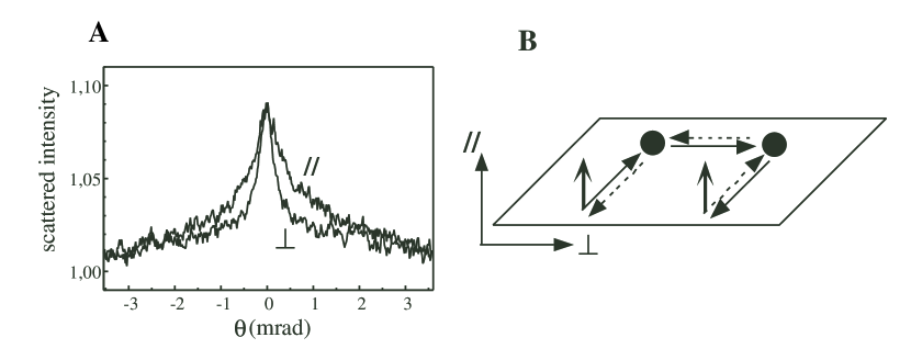
Figure 17: Anisotropy of the CBS cone in the $lin$ $//$ $lin$ channel. A : cone cross-sections parallel and orthogonal to the incident polarization B : origin of the anisotropy.

This effect, which has already been reported with classical Rayleigh scatterers[9], is due to the combination of low scattering orders and a dipole-type radiation pattern for the atomic scatterer. Indeed, if we consider for instance only double scattering and an incident vertical linear polarization, most of the scattering paths will lie in the horizontal plane because very little light will be radiated in the vertical direction (fig 17B). Thus, the phase difference between reverse paths will vary much more slowly in the vertical angular direction (where the detector moves along a fringe of the equivalent Young’s interference pattern) than in the horizontal one (motion orthogonal to the fringe system), yielding an asymmetric cone. A model including only double scattering (for a semi-infinite medium) by atoms with an internal structure yields a cone with an asymmetry close to the experimental observation. Since this effect originates essentially from the lowest scattering orders, this agreement is not surprising.

5 Conclusion

In this paper, we discussed in details our experiment of coherent backscattering of light from cold atoms. A particular attention was drawn to the influence of sample and laser probe geometry on the CBS signal, as illustrated by experiments on classical samples. The small enhancement factors observed in the experiment on cold atoms are explained by two effects due to the atom’s internal structure : the presence of single scattering (spontaneous Raman transitions), and a more interesting imbalance effect in the amplitudes of the time-reversed paths. We are currently setting up a Monte Carlo simulation to take into account the specific geometry of our sample together with the internal structure properties of the atomic scatterer. Once this necessary tool is developed, we plan to quantitatively study the effect of various parameters such as different atomic transitions, laser frequency and intensity, or an applied magnetic field.

Acknowledgement: We thank the CNRS and the PACA Region for financial support. We gratefully acknowledge the important contributions of D. Delande and T. Jonckheere to the theoretical work and numerical simulations, and of J.-C. Bernard to the development of the experiment.

References

- [1] P.W. Anderson, Phys. Rev. 109, 1492-1505 (1958).
- [2] A.Z. Genack & N. Garcia, Phys. Rev. Lett. 66, 2064-2067 (1991).
- [3] D.S. Wiersma, P. Bartolini, A. Lagendijk & R. Righini, Nature 390, 671-673 (1997).
- [4] Y. Kuga & A. Ishimaru, J. Opt. Soc. Am. A 8 831 (1984); P.E. Wolf & G. Maret, Phys. Rev. Lett. 55, 2696 (1985); M.P. van Albada, A.Lagendijk, Phys. Rev. Lett. 55, 2692 (1985); K.M. Yoo, G.C. Tang & R.R. Alfano, Appl. Opt. 29, 3237-3239 (1990); M.I. Mishchenko, Astrophys. J. 411, 351-361 (1993); D.S. Wiersma, M.P. van Albada, B.A. van Tiggelen & A. Lagendijk, Phys. Rev. Lett. 74, 4193-4196 (1995); A. Tourin, A. Derode, P. Roux, B.A. van Tigelen & M. Fink, Phys. Rev. Lett. 79, 3637-3639 (1997).
- [5] G. Labeyrie, F. de Tomasi, J.-C. Bernard, C. A. Müller, C. Miniatura & R. Kaiser, Phys. Rev. Lett. 83 5266 (1999).
- [6] D.W.Sesko, T.G.Walker, C.E.Weiman, J. Opt. Soc. Am. B 8, 946 (1992).
- [7] A. Fioretti, A.F. Molisch, J.H. Muller, P. Verkerk & M. Allegrini, Optics Comm. 149, 415-422 (1998).
- [8] E. Akkermans & R. Maynard, J. Phys. (Paris), Lett. 46, L-1045 (1985).
- [9] M. P. van Albada, M. B. van der Mark & A. Lagendjik, Phys. Rev. Lett. 58, 361 (1987).
- [10] D. Wiersma, M. van Albada, B. van Tiggelen & A. Lagendijk, Phys. Rev. Lett. 74, 4193 (1995).
- [11] M. B. van der Mark, M. P. van Albada, & A. Lagendjik, Phys. Rev. B 37, 3575 (1988).
- [12] B. A. van Tiggelen, A. Lagendijk & A. Tip, J. Phys. : Condens. Matter 2, 7653-7677 (1990).
- [13] Murty M., Appl. Opt. 3 (1964) 531.
- [14] D.S. Wiersma, M. P. van Albada, & A. Lagendijk, Rev. of Scient. Instrum. 66 5473 (1995).
- [15] B. A. van Tiggelen, and R. Maynard, in Wave Propagation in Complex Media, ed. G. Papanicolaou, IMA Vol. 96 (Springer, New York, 1997).
- [16] Mishchenko M. I., J. Opt. Soc. Am. A 9 no.6 (1992).
- [17] F.C. MacKintosh, J.X. Zhu, D.J. Pine, D.A. Weitz, Phys. Rev. B 40 9342 (1989).
- [18] R. Lenke & G. Maret in Scattering in Polymeric and Colloidal Systems, eds. W. Brown and K. Mortensen (Gordon and Breach, Reading U.K.) (in press).
- [19] T. Okamoto & T. Asakura, Optics Lett. 21 369 (1996).
- [20] A. A. Golubentsev, Sov. Phys. JETP 59 , 26 (1984).
- [21] A. Lagendijk & B.A. van Tiggelen, Phys. Reports 270 167 (1996) .
- [22] T. Jonckheere, C. A. Müller, R. Kaiser, C. Miniatura, & D. Delande, submitted to Phys. Rev. Lett. (2000).
- [23] A. Ishimaru, in Wave Propagation and Scattering in Random Media (Academic, New York, 1978), Vols. I and II.