A Two-Species Exclusion Model With Open Boundaries: A use of -deformed algebra
Farhad H Jafarpour ***e-mail:JAFAR@theory.ipm.ac.ir
Department of Physics, Sharif University of Technology,
P.O.Box 11365-9161, Tehran, Iran
Institute for Studies in Theoretical Physics and Mathematics,
P.O.Box 19395-5531, Tehran, Iran
In this paper we study an one-dimensional two-species exclusion model
with open boundaries. The model consists of two types of particles moving
in opposite directions on an open lattice. Two adjacent particles swap
their positions with rate and at the same time they can return to
their initial positions with rate if they belong to the different
types. Using the Matrix Product Ansatz (MPA)
formalism, we obtain the exact phase diagram of this model in restricted
regions of its parameter space. It turns out that the model has two
distinct phases in each region. We also obtain the exact expression for
the current of particles in each phase.
PACS number: 05.60.+w , 05.40.+j , 02.50.Ga
Key words: Asymmetric Simple Exclusion Process (ASEP), Partially Asymmetric Simple Exclusion Process (PASEP), Matrix Product Ansatz (MPA)
I Introduction
The stationary state properties of one-dimensional driven diffusive
systems are currently of much research interest [1-5]. These systems
exhibit very interesting cooperative phenomena such as boundary-induced
phase transitions,
spontaneous symmetry breaking and single-defect induced phase transitions
which are absent in one-dimensional equilibrium statistical mechanics. Many
physical phenomena such as hopping conductivity, growth processes and traffic
flows can also be explained by these models [6-9]. One of the most basic
model is the Asymmetric Simple Exclusion Process (ASEP), which shows a rich
behavior [10].
The ASEP is a model of particles diffusing on a lattice driven by an external
field and
with hard-core exclusion. Models with more than one kind of particles have
also been investigated. The ASEP in the presence of a second class particle
(impurity) has provided a framework for the study of shocks (see [5] and
[9]). Another model of this kind is the Partially Asymmetric Simple
Exclusion Process (PASEP). In this model, particles are allowed to hop
both to their immediate right and left sites with unequal rates. This
model has been studied both with open boundaries [20] and in the presence
of an impurity on a ring [11].
A multi-species ASEP has also been suggested, which seems to be a simple
realization for real traffic [12].
In this paper we consider a model containing two types of particles on a
lattice of length with open boundary condition. The two types of particles,
which we refer to them as ” positive ” and ” negative ” particles, move in
opposite direction. The positive (negative) particles are injected (removed)
from the left-most site of the lattice and are removed (injected) from the
right-most site of the lattice. Every where through the lattice, two
adjacent particels
interchange their positions, unless they are both positive or negative.
The system evolves according to an stochastic
dynamical rule as follows. In each infinitesimal time step the following
events occur at each nearest-neighbour pair of sites
:
| (1) | |||
| (2) | |||
| (3) | |||
| (4) |
where and indicate a positive or a negative particle,
respectively, and indicates an empty site.
Also, in each infinitesimal time step , the following events may occur
at the first and the last site of the lattice:
| (7) | |||||
| (10) |
For , this model reduces to the model introduced in [13,14]
which using simulation data and doing exact calculations has been
extinsively studied. These authors
have shown that for certain values of the parameters and
the symmetry of dynamics under interchange of positive and negative particles
and of their directions is spontaneously broken.
In reference [15] Alcaraz et al have studied the -species stochastic
models with open boundary and found their related algebras, which appear
in
the MPA formalism first introduced in [16]. Our model can be considered as
a case which will be studied in details.
The process has also been considered on a closed ring in [17-19]. It
has been shown that when the density of positive particles is equal to
the density of negative ones, depending on the values of the parameters
of the model, three phases exist: a pure
phase in which one has three pinned blocks of only positive, negative particels
and vacancies (where the translational invariance is spontaneously
broken);
a mixed phase with a non-vanishing current of particles; and a disordered
phase.
Here we study the effects of the open boundaries. For certain cases
or we are able to solve our model exactly and find the
modified phase diagrams (in comparison with case). We will show that
for , where the system is devoid of vacancies, only two phases
exist. In limit the model has also two distinct phases in which the
current of positive particles is equal to those of negative ones.
This paper is organized as follows. In section we will present the
exact solution of the model for the case using the known
results. We will also obtain the exact generating function of the
partition
function of the model using the Matrix Product Ansatz (MPA) and calculate
the current of the particles in limit. In the last section we will
compare our results with those obtained in [13] for .
II Matrix Product Solutions
In this section we will show that the stationary probability of the model
defined in and can be obtained using the MPA
for two specific cases and . According to the MPA
formalism, the stationary probability of any configuratin
can be written as a matrix element of a product of non-commuting
operators.
Before reviewing this approach we define some notations. We introduce two
occupation numbers, and , for each site , where
if site is occupied by a positive particle and otherwise.
Similarly, if site is occupied by a negative particle and
otherwise. Since the process is exclusive, so that each site of the
lattice can only be occupied at most by one particle, each configuration of
the system is uniquely defined by the set of occupation numbers
. Now the normalized stationay state weight for a
lattice of size can be witten as:
| (11) |
The normalization factor in the denominator of the equation ,
which plays a role analogous to the partition function in equilibrium
statistical mechanics, is a fundumental quantity and can be calculated using
the fact . Thus
one finds
| (12) |
in which . The operators , and correspond to the presence
of a positive, a negative particle, and a hole respectively. These
operators with the vectors
and satisfy a certain algebra which will be
discussed below.
A The limit
In this limit, as soon as a hole appears at a boundary site, it is
removed. Therefore in the steady state the lattice will be empty of
holes. Now the dynamical rules given by and reduce to
| (13) | |||
| (14) | |||
| (15) | |||
| (16) |
Using the MPA one obtains the following quadratic algebra for this case
| (17) | |||||
| (18) | |||||
| (19) |
Now if one imagine the negative particles as holes, the problem reduces
to the single-species PASEP
with open boundaries and equal injection and extraction rates.
As we mentioned, recently
the PASEP has been studies widely with open boundaries [20]. Using
the results given there, we find two following phases in
the thermodynamic limit :
The current of the positive particels is equal to the current of the
negative ones and has its maximum value
| (20) |
Also the density of the positive particles in the bulk has a
power law behavior
| (21) |
The density of the negative particels can be obtained using the
equality .
The current of the positive particels is again equal to the
current of the negative ones and is given by
| (22) |
The density profile of the positive particles is linear in the bulk which is
a consequence of the superposition of shocks
| (23) |
This phenomenon has also been observed in the ASEP with open boundaries when the injection and extraction rates become equal [10].
B The limit
Another limit which can be solved using the MPA formalism exactly is
.
The operators and vectors satisfy the following algebra
| (24) | |||||
| (25) | |||||
| (26) | |||||
| (27) | |||||
| (28) | |||||
| (29) | |||||
| (30) |
Following [13] one can choose
| (31) |
Then the algebra can be written as
| (32) | |||||
| (33) | |||||
| (34) |
This algebra is very similar to the algebra associated with the PASEP [19,20]. Here
we adopt the same representation proposed in [19]. One can easily check
that the following representation satisfy and
| (35) |
Where the superscript indicates the transpose,
| (36) |
and .
Using the matrix algebra given by and we find the following
expressions for the current of the positive and the negative particles in the
stationary state
| (37) | |||
| (38) |
As can be seen from , the currents are site-independent (as it
should be
in the stationary state), equal and given by the matrix element of powers of .
In what follows we will introduce a generating function to calculate the matrix
element of all powers of betwen the vectors and
.
Define a generating function
| (39) |
The convergence radius of this formal series, , is proportional to the
current of particles given by in the thermodynamic limit
| (40) |
On the other hand, the radius of convergence is the absolute value of the
nearest
singularity of to the origin. Once we obtain the singularities
of the function , we can calculate the current of particles and
distinguish the phases.
Using and one can expand the expression
as
| (41) |
where . Noting that , after some computation, we obtain
| (42) |
and also
| (43) |
It is known that the expression
can be written
explicitly in terms of the basic -hypergeometric function (see [19]
and references therein)
| (44) |
in which . The quantities and are defined as
| (47) | |||||
| (48) |
Lastly, the basic -hypergeometric function is defined by the series
| (49) |
which tends to the usual hypergeometric series as . The
series converges when and [20]. In this paper
the convergence condition of is ; therefore, without losing
the generality, we limit ourselves to this region.
As we mentioned, the singularities of specify the phase diagram
of the model. From the expression , we see that there are two possible
sources for the singularities: the singularities of and a zero
of the denominator of . First we consider the singularities of
. From one can see that has two
singularities:
which is a square root singularity and
which is a simple root. In order to
discuss the zeros of the denominator of , we use the same assumption
proposed in [19]. In the convergence region of i.e. , for
the function satisfies . It means that the
function increases monotonically from to when ;
therefore, the equation (which gives the zeros of the
denominator
of ) has only one root in this region. Comparing the absolute value of the
singularities , and , one can easily
find the following results:
For the radius of convergence of the formal
series is equal to which is the
solution of the equation .
Since is a simple pole, we expect that behaves
asymptotically as .
The current of the particles can also be obtained
| (50) |
For two different situations may occur.
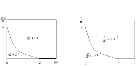
In the region specified by and , we find
and the current of particles to be
| (51) |
In the region , it turns out that
which is again the solution of the equation . The
partition function again behaves as and the current
of particles in this case can be obtained from . The boundary of
these two recent phases will be specified by
| (52) |
In Fig.1 we have plotted the phase diagram of our model in limit both for (the left diagram) and (the right diagram). As we mentioned in section (2) for , the line is the line of shock configurations. The bold lines in Fig.1 mark these lines.
III Comparison and Concluding Remarks
In this paper we studied a generalized two-species exclusion model
with open boundaries. The positive particles are supplied at the left end
of the chain and they leave it at the right end. Similarly, the negative
particles are supplied at the right end and they leave the system at the left
end. As soon as a positive and a negative particle meet each other (the positive
particle is supposed to be in the left hand side of the negative
particle), they
interchange their positions with rate . At the same time they may go to their
initial positions with rate . In limit this model reduces to the
one studied in [13]. Using the MAP formalism, our model has been
studied in two
different limits ( and ) and the corresponding phase
diagrams obtained. It has been shown that all the phases are symmetric in which
the current of the positive and negative particles are equal. One can easily
check that for all the results obtained here reduce to those obtained
in [13]. In comparison with [13], as can be seen in Fig.1, the phase
diagram of the model has been modified.
The study of the whole parameters space of the model proposed in this paper
is still an open problem. Using the mean field approximation and simulation
data,
the authors have shown that in limit this model has also asymmetric
phases where the current of the positive and negative particles become
different. It will be interesting to study the structure of asymmetric phases
of this model which may occur for the certain values of the parameters ,
, and .
Acknowledgement:
I would like to thank V. Karimipour for reading the manuscript.
REFERENCES
- [1] T. M. Ligget, Intracting Particle Systems (Springer-Verlag, New York, 1985).
- [2] T. M. Ligget, Stochastic Intracting Systems: Contact, Voter, and Exclusion Processes (Springer-Verlag, New York, 1999).
- [3] H. Spohn, Large Scale Dynamics of Intracting Particles (Springer-Verlag, New York,1991).
- [4] B. Schmittmann and R. K. P. Zia, Statistical mechanics of driven diffusive systems, in Phase Transitions and Critical Phenomena, Vol 17, C. Domb and J. Lebowitz eds. (Academic, London, 1994).
- [5] K. Mallick, Shocks in the asymmetry exclusion model with an impurity, J. Phys. A: Math Gen. 29, 5375 (1996).
- [6] P.M. Richards, Theory of one-dimensional hopping conductivity and diffusion, Phys. Rev. B 16, 1393 (1977).
- [7] K. Nagel and M. Schreckenberg, J. Phys. I France 2, 2221 (1992).
- [8] J. Krug, Boundary induced phase transition in driven diffusive systems, Phys. Rev. Lett. 67, 1882 (1991).
- [9] H-W. Lee, V. Popkov and D. Kim, Two way traffic flow: Exactly solvable model of traffic jam, J. Phys. A: Math Gen. 30, 8497 (1997).
- [10] B. Derrida, An exactly soluble non-equilibrium system: The asymmetric simple exclusion model, Phys. Rep. 301, 65 (1998).
-
[11]
F. H. Jafarpour, Partially asymmetric simple
exclusion model in the presence of an impurity on a ring, J. Phys. A: Math Gen. 33,
1797 (2000),
T. Sasamoto, One-dimensional partially asymmetric simple exclusion process on a ring with a defect particle, cond-mat/9910483 and also [5]. - [12] V. Karimipour, A multi-species asymmetric simple exclusion process and its relation to traffic flow Phys. Rev. E 59, 205 (1999).
-
[13]
M. R. Evans, D.P. Foster, C. Godreche and
D. Mukamel, Asymmetric exclusion model with two species: Spontaneous
symmetry breaking, J. Stat. Phys. 80, 69 (1995) and
M. R. Evans, D.P. Foster, C. Godreche and D. Mukamel, Spontaneous symmetry breaking in one dimensional driven diffusive system, Phys. Rev. Lett. 74, 208 (1995). - [14] P.F. Arndet, T. Heinzel and V. Rittenberg, First-order phase transitions in one-dimensional steady states, J. Stat. Phys. 90, 783 (1998).
- [15] F. C. Alcaraz, S. Dasmahapatra and V. Rittenberg, N-species stichastic models with boundaries and quadratic algebras, J. Phys. A: Math Gen. 31, 845 (1998).
- [16] B. Derrida, M.R. Evans, V. Hakim and V. Pasquier, Exact solution of a 1d asymmetric exclusion model using a matrix formulation, J. Phys. A: Math Gen. 26, 1493 (1993).
- [17] P.F. Arndet, T. Heinzel and V. Rittenberg, Spontanious breaking of translational invariance and spatial condensation in stationary states on a ring, J. Stat. Phys. 97, 1 (1999).
- [18] P.F. Arndet, T. Heinzel and V. Rittenberg, Spontaneous breaking of translational invariance in one-dimensional stationary states on a ring: The neutral system, J. Phys. A: Math Gen. 31, L45 (1998).
- [19] N. Rajewsky, T. Sasamoto and E. R. Speer, Spatial particle condensation for an exclusion process on a ring, cond-mat/9911322.
- [20] T. Sasamoto, One-dimensional partially asymmetric simple exclusion model with open boundaries: Orthogonal polynomials approach, J. Phys. A: Math Gen. 32, 7109 (1999).