[

Boundary induced phase transitions in driven lattice gases with meta-stable states

Abstract

We study the effect of meta-stability onto boundary induced phase transitions in a driven lattice gas. The phase diagram for open systems, parameterized by the input and output rates, consists of two regions corresponding to the free flow and jammed phase. Both have been entirely characterized. The microscopic states in the high density phase are shown to have an interesting striped structure, which undergoes a coarsening process, and survives in the thermodynamic limit.

]

Driven lattice gases (DLG) are characterized by a non-vanishing mass-flow in the stationary state which is generated by non-potential forces [1]. This feature of DLG has far reaching consequences, because even the stationary state of the system is not described in the framework of standard equilibrium statistical mechanics [2]. In recent years the study of various non-equilibrium lattice gas models, which have important applications, e.g. in biological context [3] or as models for traffic flow [4, 5], led to a profound understanding of some key features of systems far from equilibrium.

One of the most fascinating effects observed for this kind of models are so-called boundary induced phase transitions, i.e. the change of the bulk properties due to a variation of the boundary conditions [6, 7]. Such phase transitions have been extensively studied for a class of 1D DLG with a continuous flow density relation for periodic boundary conditions (PBC). For some models even exact results for the stationary state exist [8, 9, 10]. A phenomenological theory [11] was recently able to predict the phase diagram in the case of open boundary conditions (OBC) also for more complicated models [12]. However, less is known for DLG which exhibit meta-stable states for PBC [13], although they are relevant in different fields. Here, we study one of the simplest DLG model which shows meta-stability for PBC. We first discuss briefly the case of PBC, but our main focus is to study the effect of meta-stability in the case of OBC. Using a combination of analytical and numerical methods we explore the structure of the phase diagram and characterize the typical behavior in the different phases.

We study a DLG model defined on a chain of length $L$. Each site of the chain may either be empty ($x$) or occupied with a particle of velocity zero ($0$) or one ($1$). In a first step all particles which moved in the previous time step keep their velocity if the next site is empty. With probability $q_{0}$, velocity one is assigned to particles with velocity zero and an empty site ahead. In all other cases velocity zero is assigned to the particle. In the second step particles with velocity one move to the next site. Both steps are applied synchronously to all particles.

This model may be interpreted as a special case of the recently introduced VDR model for traffic flow [13], i.e. we restrict the maximal velocity of the particles to one. For $q_{0}=1$ we recover the deterministic asymmetric exclusion process with parallel dynamics [10].

FIG. 1.: Flow density relation for PBC with $q_{0}=0.25$ and $L=1,000$. Empty circles show simulation results for an initialization where all particles have velocity one and at least one empty site in front. Filled circles show results starting the simulation with a compact cluster of particles. These results are compared to our estimate for $L\to\infty$ (solid line).

Following [11], the structure of the flow-density relation, i.e. the fundamental diagram, in the case of PBC is a key to understand the behavior of the open chain. Fig. 1 shows the numerically established fundamental diagram for our model, in comparison with:

$$J(\rho) = \rho\quad\text{ if }0\leq\rho\leq 0.5$$

$$J(\rho) = q_{0}(1-\rho)\quad\text{ if }q_{0}/(1+q_{0})\leq\rho\leq 1$$

The form of the fundamental diagram can be easily understood. For densities $0\leq\rho\leq 0.5$ and suitable initial configurations (the initial velocity of the particles is one and no particle is blocked) all particles move deterministically with velocity one. At larger densities $\rho>0.5$ the number of particles exceeds the number of holes, i.e. one cannot avoid the formation of clusters of particles. The simulation results indicate that in the steady state one observes phase separation, i.e. the formation of a large compact cluster of particles which coexists with a free-flow regime. The density in the free-flow regime is determined by the frequency of particles leaving the cluster. The typical time the first particle needs to separate from the cluster is simply given by $T=q_{0}^{-1}$. This time already determines the average gap between two particles in the low-density regime. Therefore the average density, $\rho_{free}$ in the free-flow regime is given by $\rho_{free}=1/(T+1)=q_{0}/(1+q_{0})$. The number of moving particles and therefore the flux follows from particle conservation (see also [13]).

Both solutions for $J(\rho)$ coexist for $\rho_{free}\leq\rho\leq 1/2$. For finite systems it is possible that the large cluster dissolves due to fluctuations. In free flow states, fluctuations are absent and therefore no spontaneous cluster formation takes place at densities $\rho\leq 0.5$. However, in the thermodynamic limit, any random initial configuration leads to a jammed stationnary state.

After this short discussion of the system with PBC, we proceed with the open chain. OBC are implemented as follows : at the left boundary particles with velocity one are introduced with probability $\alpha$ if the first site of the chain is empty. At the right end the particles leave the chain from site $L$ with probability $\beta$, irrespective of their velocity.

The values of $\alpha$ and $\beta$ determine for given values of $L$ and $q_{0}$ the bulk behavior of the system. First we notice that for $\beta=1$ the only stochastic element is due to the left boundary, i.e. we recover the deterministic asymmetric exclusion process. Therefore the exact result for the flow [10] is given by $J(\alpha)=\alpha/(1+\alpha)$. This result for the flow is expected to be valid not only for $\beta=1$ but in the whole low density phase, because for low bulk densities the flow is controlled by the input of particles.

Next, we consider the case of large bulk densities, i.e. we study the system’s performance for large values of $\alpha$ and $\beta\ll 1$. For this case we expect to find frequently a compact cluster of particles at the right boundary. Therefore the mean time interval for a particle leaving the system is the sum of the average waiting time $T_{L}=1/\beta$ of the last particle at site $L$ and the average time which passes until the last site is occupied again, $T_{J}=1/q_{0}$. We find immediately that for large $\alpha\approx 1$ and $\beta\ll 1$ the flow is given by

$$J(\beta)=\frac{1}{T_{L}+T_{J}}=\frac{q_{0}\beta}{q_{0}+\beta}.$$ (1)

FIG. 2.: Comparison of the estimated flow with simulation results. The simulation results have been obtained for a chain of length $L=500$ and $q_{0}=0.25$. (a) The Figure shows the perfect agreement of simulation results and the estimate $J(\alpha)$. We used $\beta=1.$ and $\beta=0.5$ as output probabilities. (b) $\beta$ dependence of the flux ($\alpha=0.5$). The estimated flux and the simulation results agree for sufficiently small values of $\beta$. Simulations for different lengths of the chain indicate that the deviations for $\beta$ near one are due to finite size effects.

This simple scenario is only valid if the density of holes fed into the system is very low. For larger values of $\beta$ we expect that it is also possible that the cluster separates from the right boundary. In this case the density close to the exit is determined by the outflow from a cluster. The temporal headway $t$ between two consecutive particles is distributed via $P_{h}(t)=q_{0}(1-q_{0})^{t-1}$ where $t\geq 1$. Now we calculate the typical amount of time which is needed from the arrival of a particle (at $t=0$) to the arrival of the second particle at ($t=T$) at site $L$. Here we have to distinguish two cases: $(i)$ the particle arrives at site $L-1$ before the first particle has left the system or $(ii)$ that it arrives later, such that it reaches the last site without being blocked by the particle ahead. The probability that a particle gets blocked if it arrives at $t$ is given by $P_{b}(t)=(1-\beta)^{t}$ and that it can pass without blockage by $P_{f}(t)=\sum_{\tau=1}^{t}\beta(1-\beta)^{t-1}$.

This leads to the average value of $T$ given by

$$T = \sum_{t=1}^{\infty}P_{h}(t)\left[P_{f}(t)(t+1)+P_{b}(t)(t+\frac{1}{\beta}+\frac{1}{q_{0}})\right]$$ (2)

$$= \frac{1}{\beta}+\frac{1}{q_{0}}=J(\beta)^{-1}.$$ (3)

Also for this scenario we recover the same value (1) of the flow. These two kind of configurations are generic if the output probability controls the capacity of the system, i.e. in the presence of clusters. Therefore we expect to find a unique functional dependence of the flow, if the system is controlled by the capacity of the exit. The transition between the $\alpha$ or $\beta$ controlled parameter regime is expected to be located at

$$\beta_{t}(\alpha)=\frac{q_{0}\alpha}{(1+\alpha)q_{0}-\alpha}$$ (4)

where both fluxes agree.

Comparison of our prediction for the flow with simulation results shows excellent agreement (see fig. 2). Simulations for different lengths of the chain show that the differences between our predictions and the simulations systematically vanish for larger system sizes. The origin of these finite size effects, i.e. the enhancement of the flow for large $\beta$, is the possibility to find occasionally cluster-free micro-states. We indicated this by the broken lines in the phase diagram (Fig. 4). The absence of maximal current phase in the thermodynamic limit is related to the non-analyticity of the fundamental diagram [11].

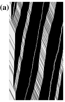
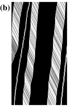
FIG. 3.: Typical space-time plots in the striped phases. The figure shows the first $\sim 400$ sites of a chain of length $L=1,000$. (a) For $SPI$ the size of the last clusters decreases rapidly close to the entrance. ($\alpha=0.1,\beta=0.1,q_{0}=0.4$) (b) For $SPII$ the efficient particle reservoir at the entrance of the system augments the size of the leftmost cluster.

FIG. 4.: Phase diagram of the open system for $q_{0}=0.25$. The phases are in order: low density phase (LD), striped phase I (SPI), and striped phase II (SPII). At the line $\alpha=q_{0}$ one observes a constant density profile. The dashed lines show parameter regimes where in finite systems a systematically larger flux has been observed.

We proceed characterizing the typical microscopic structure of the stationary state, in different parameter regimes. We distinguish three different domains, i.e. a low density domain (LD) for $\beta>\beta_{t}(\alpha)$ (LD), and two high density domains for $\beta<\beta_{t}(\alpha)$. Both high density domains correspond to a striped phase (SP), but they exhibit different behaviors in the vicinity of the entrance, depending whether $\alpha<q_{0}$ (SPI) or $\alpha\geq q_{0}$ (SPII). In the LD phase we observe the typical two domain structure known from the asymmetric exclusion process. Clusters which eventually separate from the high density domain at the right dissolve in a few time steps. This dissolution leads to the localization of the high density domain at the right. The system takes a bulk density $\rho_{b}(\alpha)=J(\alpha)$. At site $L$ the density is given $\rho_{L}=J(\alpha)/\beta$. Fits of several density profiles follow the pure exponential form $\rho(n)=\rho_{b}(\alpha)+[\rho_{L}-\rho_{b}(\alpha)]\exp(-(L-n)/\xi)$.

In the high density region (SPI + SPII), clusters are able to reach entrance. This region can be described by considering that at the right boundary, some free-flow segments are injected within a compact cluster. Typically, the free-flow segments reduce to isolated holes for $\beta<q_{0}$, whereas for $\beta>q_{0}$, they contain both empty sites and particles with velocity one. Both the free-flow segments and the compact clusters separating them move backwards, producing a striped structure in spatio-temporal plots (see fig. 3). As long as it is far enough from the left boundary, a cluster has the same in- and output rates, thus its width follows a non-biased random walk, whose average is a constant. However, there is a non-vanishing probability that the width of the cluster crosses the zero value, leading to the coalescence of the two neighboring free-flow segments, which will never be able to separate again afterwards. The excess particles are distributed among the neighboring clusters. Thus, as the stripes move towards the entrance, their widths increase. However, the average density remains a constant equal to the density selected on the left boundary $\rho=J(\beta)/\beta$. When the clusters arrive near the left boundary and are exposed to the entrance flux, their width suddenly obeys a biased random walk. If $\alpha>q_{0}$ (phase SPII), the width increases on average and the high input rate stabilizes the cluster until it reaches the boundary (fig. 3-b). If clusters and free-flow segments at a given position were monodisperse, then the sudden rate change would induce a linear density profile on the left, with a crossover to the constant bulk value occurring at site $\tilde{n}=\alpha t_{f}/(1+\alpha)$ where $t_{f}$ is the average time interval during which free-flow is observed in the first site, i.e. the typical time between the disappearance of a jam and the arrival of the next. Due to the coarsening of the striped pattern in upstream direction one observes a subextensive growth of $t_{f}$ with increasing system size. The density in the first site is determined by noticing that the flux (1) is also equal to $j=\alpha(1-\rho_{1})$. If we measure $t_{f}$ numerically, we find a quite good agreement between our estimate and the measured density profile (see fig. 5), except that the crossover region is in fact very large due to size dispersion of clusters and free-flow segments.

FIG. 5.: Density profile in the SPII region. The numerical result (solid line) is compared with the theoretical prediction (dashed line) based on an assumption of monodispersity and parameterized by $t_{f}$ which has to be determined numerically.

If $\alpha<q_{0}$ (phase SPI), the width of the leftmost cluster decreases on average due to the reduced capacity of the entrance. Some clusters will even not be able to reach the entrance, as seen on fig. 3. As long as we are far from the transition line $\beta_{t}(\alpha)$, still, clusters are on average large enough so that most of them reach the entrance and the depletion region remains localized on the left. The calculation done in SPII for the density profile is still valid. The only difference is that now the linear part has a positive slope. However, as we approach the transition line $\beta_{t}(\alpha)$, more and more clusters do not reach the boundary. When a given cluster disappears before reaching the left end, the next one is exposed earlier to the low incoming flux, and thus the depletion region may invade the whole system. The line separating the depletion region from the constant density region becomes delocalized over the whole system as the transition line is approached.

To conclude, we analyzed a DLG exhibiting meta-stable states. The structure of the phase diagram was explored by simulations as well as by a phenomenological description. The analytical predictions for each phase agree extremely well with the simulation results. The most characteristic feature is the spontaneous formation of simultaneously existing clusters for restricted outflow. The coarsening of these clusters as they flow backwards is due to the stochasticity of the model. We stress that this striped pattern survives in the thermodynamic limit. We expect that this behavior and more generally the structure of the phase diagram are generic for DLG with branched fundamental diagrams - this branched structure being a signature of meta-stability. Moreover we established, in the limit of large system size, the absence of a maximal current phase.

Besides a phenomenological similarity with the clogging phenomena in granular flow [16], the practical relevance can be illustrated by the example of traffic flow, where the importance of boundary induced phase transitions is well accepted [14]. Although we chose a rather simplistic model and do not aim to give a complete description of traffic flow, our results can be related to experimental studies that revealed the existence of parallel existing clusters on highways [15]. These experimental results now can be directly related to the existence of meta-stable states. Moreover, our result shows that jams can be observed far upstream even when boundary induced. Another interesting feature are the important finite size effects, which probably can be used for a systematic flow optimization [17].

Acknowledgments: We thank Robert Barlovic, Andreas Schadschneider, and J. Krug for useful discussions. L. S. acknowledges support from the Deutsche Forschungsgemeinschaft under Grant No. SA864/1-1.

REFERENCES

- [1] B. Schmittmann and R.K.P. Zia, in: Phase Transitions and Critical Phenomena, Vol. 17, eds. C. Domb and J.L. Lebowitz (Academic Press, 1995)
- [2] G.M. Schütz, in: Phase Transitions and Critical Phenomena, eds. C. Domb and J.L. Lebowitz (to appear)
- [3] J.T. MacDonald and J.H. Gibbs, Biopolymers 7, 707 (1969)
- [4] K. Nagel and M. Schreckenberg, J. Physique I, 2, 2221 (1992)
- [5] D. Chowdhury, L. Santen, and A. Schadschneider, Physics Reports 329, 199 (2000)
- [6] J. Krug, Phys. Rev. Lett. 67, 1882 (1991)
- [7] V. Popkov, L. Santen, A. Schadschneider, and G.M. Schütz, preprint, cond-mat/0002169 (2000)
- [8] G.M. Schütz and E. Domany, J. Stat. Phys. 72, 277 (1993), B. Derrida, M.R. Evans, V. Hakim, and V. Pasquier, J. Phys. A 26, 1493 (1993)
- [9] A. Honecker and I. Peschel, J. Stat. Phys. 88, 319 (1997); N. Rajewsky, L. Santen, A. Schadschneider, and M. Schreckenberg, J. Stat. Phys. 92, 151 (1998)
- [10] M.R. Evans, N. Rajewsky and E.R. Speer, J. Stat. Phys. 95, 45 (1999); J. de Gier and B. Nienhuis, Phys. Rev. E 59, 4899 (1999)
- [11] A.B. Kolomeisky, G.M. Schütz, E.B. Kolomeisky, and J.P. Straley, J.Phys. A 31, 6911 (1998)
- [12] V. Popkov and G. Schütz, Europhys. Lett. 48, 257 (1999)
- [13] R. Barlovic, L. Santen, A. Schadschneider, and M. Schreckenberg, Eur. Phys. J. 5, 793 (1998)
- [14] H.Y. Lee, H.-W. Lee, and D. Kim, Phys. Rev. Lett. 81, 1130 (1998), D. Helbing, A. Hennecke, and M. Treiber, Phys. Rev. Lett. 82, 4360 (1999), M. Treiber, A. Hennecke, and D. Helbing, To appear in Phys. Rev. E 62, (August 2000).
- [15] B.S. Kerner and H. Rehborn, Phys. Rev. E 53, R4275 (1996)
- [16] T. Pöschel, J. Phys. I France 4, 499 (1994)
- [17] R. Barlovic, diploma thesis Duisburg (1998).