Crossover from the chiral to the standard universality classes in the conductance of a quantum wire with random hopping only

Abstract

The conductance of a quantum wire with off-diagonal disorder that preserves a sublattice symmetry (the random hopping problem with chiral symmetry) is considered. Transport at the band center is anomalous relative to the standard problem of Anderson localization both in the diffusive and localized regimes. In the diffusive regime, there is no weak-localization correction to the conductance and universal conductance fluctuations are twice as large as in the standard cases. Exponential localization occurs only for an even number of transmission channels in which case the localization length does not depend on whether time-reversal and spin rotation symmetry are present or not. For an odd number of channels the conductance decays algebraically. Upon moving away from the band center transport characteristics undergo a crossover to those of the standard universality classes of Anderson localization. This crossover is calculated in the diffusive regime. Numerical simulations agree qualitatively with the theory.

PACS numbers: 72.15.Rn, 71.30.+h, 64.60.Fr, 05.40-a

I Introduction

Since the introduction of the scaling approach to the problem of Anderson localization,[3, 4] it is known that transport characteristics of a disordered metal are universal, provided the disorder is sufficiently weak, the temperature sufficiently low so that quantum coherence is maintained over large distances, and the interaction between electrons can be neglected. An example is the phenomenon of weak localization,[5, 6] a small deviation from Ohm’s law for the conductance of a weakly disordered metal, which is suppressed by the application of a time-reversal symmetry breaking magnetic field. Though small, the weak-localization correction is universal in the sense that it does not depend on the shape of the sample, nor on any other microscopic or macroscopic property other than its dimensionality and the presence or absence of time-reversal symmetry and spin-rotation invariance. Another example is the phenomenon of universal conductance fluctuations:[7, 8] The sample-to-sample fluctuations of the conductance of a disordered metal or semiconductor are of order $e^{2}/h$ with a prefactor that only depends on dimensionality and symmetry. Both the weak-localization correction and the universal conductance fluctuations are precursors of the true Anderson localization, where as a result of destructive interference of multiple scattered quantum mechanical waves the dirty metal turns into an insulator for sufficiently strong disorder, or, in one or two dimensions, for a sufficiently large sample size.[9]

The original paper by Anderson,[10] and most of the effort devoted to the problem of Anderson localization since then, considers the case of a particle on a lattice with a random on-site potential (diagonal disorder) and non-random hopping amplitudes. In that case, one distinguishes three universality classes, corresponding to the presence or absence of time-reversal and of spin-rotation symmetry. These three classes, are called orthogonal, unitary, and symplectic, respectively. Here, we will refer to these as the three “standard” universality classes.

The electronic localization problem was soon generalized to lattice models with randomness in the hopping amplitudes (off-diagonal disorder).[11] (This type of randomness was previously known from the description of phonons[12, 13] and narrow-gap semiconductors.[14]) The localization problem with off-diagonal disorder has received comparatively much less attention, although it has been known since the work of Dyson[12] that random systems with off-diagonal disorder, but without diagonal disorder, can behave in a way dramatically different from that of systems with diagonal disorder only, or with both types of disorder.[12, 15, 16, 17, 18, 19, 20] For instance, the average density of states (DoS) for a one-dimensional chain with random nearest-neighbor hopping was found to be singular at the center of the band, $\varepsilon=0$.[12, 15, 17] According to the Thouless formula,[21] such a singular DoS implies that at $\varepsilon=0$ the conductance distribution be anomalous as well.[20, 22] Wegner and Gade in Ref. [23] (see also Refs. [18, 24, 25, 26, 27]) found a two-dimensional counterpart to the singular behavior of the average DoS within their analysis of a non-linear-$\sigma$ model with a sublattice symmetry. Interest in the effect of off-diagonal disorder has revived in the 90’s on two fronts. Motivated by quenched approximations to interacting theories such as the quantum Hall effect at half-filling or gauge approaches to high $T_{c}$ superconductivity, the random flux problem (a special case of off-diagonal disorder in which hopping amplitudes have a random phase only) has been extensively studied, although very little consensus on its localization properties has emerged.[28] A second thrust of activity has been motivated by the close resemblance between the anomalies at zero energy induced by pure off-diagonal disorder in two dimensions and the nature of the plateau transitions in the integer quantum Hall effect (IQHE):[29] Both models might share the property that all eigenstates are localized except at one special energy.[28]

The reason why the localization properties of the random hopping problem can depart from those of the standard problem of Anderson localization is the existence of an additional sublattice symmetry in systems with off-diagonal but without diagonal disorder:[18, 19, 30, 31] In that case, the lattice can be divided into two sublattices, such that the Hamiltonian changes sign under a transformation where the wavefunction changes sign on one sublattice, but not on the other. As a result, the spectrum is symmetric with respect to a reflection about $\varepsilon=0$ (i.e., eigenvalues appear in pairs $\pm\varepsilon$). The fact that the band center $\varepsilon=0$ is a very special energy in the presence of the sublattice symmetry explains why anomalies in the DoS and the localization properties occur at precisely this value of the energy. When the energy moves away from zero, the effects of the sublattice symmetry on the spectrum and the wavefunctions decreases and a crossover to the standard behavior takes place. The sublattice symmetry is broken by the presence of on-site disorder, long-range hopping,[31] or (in some cases) by periodic boundary conditions.[32] Counterparts to this sublattice symmetry in other disordered systems or in quenched approximation to interacting problems are numerous. They occur in, e.g., the QCD Hamiltonian,[33, 34] random $XY$ spin chains,[35] diffusion in random environments,[36] supersymmetric quantum mechanics,[37] non-Hermitean quantum mechanics,[38] and two-dimensional disordered models in the continuum such as Dirac fermions with random vector potentials.[39] Following previous works in this field, which adopted the nomenclature of QCD,[34] we will refer to the sublattice symmetry as chiral symmetry and will restrict our attention to random hopping problems with this symmetry.

One-dimensional disordered systems with chiral symmetry have been well-studied with all kinds of approaches and in various contexts (for references, see the previous paragraph), and despite a continuing confusion about semantics, their localization properties can be considered well-understood. For two-dimensional systems the situation is different (see Refs. [28, 40] and references therein). Reliable analytical and numerical results are notoriously hard to obtain, and no consensus has been reached to date, not even on some most elementary issues. In view of this controversy, it is particularly instructive to study the natural intermediate between one and two dimensions, the thick (or “quasi-one-dimensional”) disordered wire. On the one hand, it shares the existence of both a localized and a diffusive regime of quantum transport with two dimensional disordered systems, while on the other hand, it allows for a controllable analytic treatment, just like the truly one-dimensional system. Moreover, quasi-one-dimensional systems appear as a logical intermediate step in the finite-size scaling approach for numerical simulations in two and three dimensions.[41]

Localization properties at the band center of a quasi-one-dimensional quantum wire with off-diagonal disorder were investigated in several previous publications by the authors, together with Simons and Altland.[42, 32, 43] In those works we derived a chiral counterpart to the so-called DMPK equation,[44, 45, 46] a Fokker-Planck equation that governs the distribution of the transmission eigenvalues of a quantum wire without chiral symmetry. Solution of the chiral DMPK equation for lengths beyond the localization length of the standard DMPK equation showed that there is no exponential localization if the number $N$ of propagating channels is odd (including the one-dimensional case), while the conductance decays exponentially with length if $N$ is even. This parity effect is strikingly similar to the sensitivity of the low-energy sector of a single antiferromagnetic spin-$N/2$ chain to the parity of $N$,[47] on the one hand, or to the sensitivity of the low-energy sector of $N$ coupled antiferromagnetic spin-1/2 chains to the parity of $N$,[48] on the other hand. In the special case of the chiral Fokker-Planck equation without time reversal invariance (random phase quantum wire), it was possible to calculate exactly the crossover from the diffusive to the localized regime for all moments of the conductance and to verify the validity of the assumption of universality against a numerical simulation of the random flux problem.[32] The numerical simulations also confirmed that sufficiently far away from the center of the band, transport is governed by the standard universality classes.

A limitation of the approach relying on the Fokker-Planck equations for the transmission eigenvalues is that it cannot describe how the conductance distribution crosses over from the chiral to the standard universality class as $\varepsilon$ is tuned away from zero. In the renormalization group language, each Fokker-Planck equation describes a fixed point corresponding to a case of pure symmetry and the fixed points by themselves cannot be used to infer how the scaling flows take place between them. One possibility to obtain information about the crossover energy and length scales below (above) which the physics is that of the chiral (standard) universality classes, is to study the DoS of a chiral quantum wire.[49] However, unlike in the case of a one-dimensional wire, where the Thouless formula connects conductance and DoS, for a quasi-one-dimensional wire it is not possible to infer transport properties from the DoS. In this paper, we use an alternative approach, developed by one of us for the study of transmission through a random waveguide with absorption.[50] Focusing on weak-localization corrections and universal conductance fluctuations, we compute how, in the diffusive regime, the conductance distribution of a quantum wire with random hopping crosses over from the chiral to the standard universality classes as the energy is tuned away from zero. We are not able to compute the crossover in the localized regime. Instead, for the localized regime, we consider the conductance distributions in the pure symmetry classes and compare to numerical simulations to establish the crossover scale and to verify the validity of our predictions.

The paper is organized as follows. In Sec. II, we define our microscopic model and derive the symmetries of the scattering matrix in the presence of the chiral symmetry. We then explain the scaling approach in Sec. III. The localized regime is studied in Sec. IV. Our main results are presented in Sec. V, where we consider the crossover from the chiral to the standard universality classes in the diffusive regime. In Sec. VI we compare our theoretical predictions to a numerical simulation of a random hopping model on a square lattice. We conclude in Sec. VII.

II Microscopic model and scattering matrix

A convenient microscopic model that describes a single particle hopping randomly between two sublattices is defined. The symmetries obeyed by the scattering matrix associated to this Hamiltonian are derived. Assuming weak disorder, the microscopic model is approximated by a model defined in the continuum, for which the scattering matrix is explicitly constructed.

A Microscopic lattice model with chiral symmetry

In a general form, the Schrödinger equation for an $N$-chain system with random hopping between two sublattices and without on-site randomness reads

$$-\varepsilon\Psi^{\vphantom{{\dagger}}}(m)=T^{\vphantom{{\dagger}}}_{m}\Psi^{\vphantom{{\dagger}}}(m+1)+T^{{{\dagger}}}_{m-1}\Psi^{\vphantom{{\dagger}}}(m-1).$$ (1)

For a spinless particle, $\Psi(m)$ is the $N$-component wavefunction where the index $m$ labels the position along the chain. For a particle with spin-1/2, $\Psi(m)$ is the $N$-component wavefunction made of spinors. In that case, the $N\times N$ hopping matrix $T_{m}$ consists of quaternions.[51] The system, and the allowed hopping matrix elements are depicted in Fig. 1(a). Note that the case of a square lattice with nearest-neighbor random hopping is included in the general formula (1), see Fig. 1(b).

In order to model transport, we consider a disordered region of finite length $L=Ma$, $a$ being the lattice constant, and attach ideal leads with hopping matrix $T_{m}={\openone_{N}}$ on both ends, see Fig. 1(a). Following Refs. [42, 43], we draw the hopping matrices $T_{m}$ with $m$ inside the disordered region from a distribution centered around the $N\times N$ unit matrix,

$$T_{m}=\exp(\delta T_{m}).$$ (2)

We distinguish three symmetry classes depending on the presence or absence of time-reversal and spin-rotation symmetry. For a spinless particle (or for a spin-1/2 particle in the presence of spin-rotation symmetry), the hopping matrix $\delta T_{m}$ is real (complex) if time-reversal symmetry is present (absent). These two cases are commonly referred to as the orthogonal and unitary symmetry class and are labeled by the symmetry index $\beta=1$ and $2$, respectively. The case of broken spin-rotation symmetry with time-reversal symmetry is denoted $\beta=4$ and is referred to as the symplectic class. When $\beta=4$, the elements of the $N\times N$ matrix $\delta T_{m}$ are real quaternions.[51] The situation when both time-reversal symmetry and spin-rotation symmetry are broken reduces to the unitary class ($\beta=2$) and will not be considered separately in this paper. We further assume that $\delta T_{m}$ has a Gaussian distribution, with zero mean and with variance given by

$$\langle({\delta T_{m}})^{\vphantom{{\dagger}}}_{kl}[({\delta T_{m^{\prime}}})^{\vphantom{{\dagger}}}_{k^{\prime}l^{\prime}}]^{{\dagger}}\rangle = {2\beta a\over\gamma\ell}\delta^{\ }_{mm^{\prime}}$$ (4)

$$\mbox{}\times\left(\delta^{\ }_{kk^{\prime}}\delta^{\ }_{ll^{\prime}}-{1-\eta\over N}\delta^{\ }_{kl}\delta^{\ }_{k^{\prime}l^{\prime}}\right),$$

$$\langle({\delta T_{m}})^{\vphantom{{\dagger}}}_{kl}({\delta T_{m^{\prime}}})^{\vphantom{{\dagger}}}_{k^{\prime}l^{\prime}}\rangle = {2-\beta\over\beta}\langle({\delta T_{m}})^{\vphantom{{\dagger}}}_{kl}[({\delta T_{m^{\prime}}})^{\vphantom{{\dagger}}}_{k^{\prime}l^{\prime}}]^{{\dagger}}\rangle,$$ (5)

(6)

where

$$\gamma=\beta N+2-\beta-{2(1-\eta)\over N},$$ (7)

and $\ell$ is the mean free path. (Why $\ell$ can be identified as the mean free path is explained below.) Here, the symbol ${\dagger}$ denotes the operation of complex conjugation for $\beta=1,2$, whereas it denotes the operation of Hermitean conjugation for quaternions for $\beta=4$.[51] We assume weak disorder, $\ell\gg a$. The parameter $\eta$ governs the relative randomness of the determinant of $T_{m}$. (See Ref. [43] for the reason for its introduction.)

We have chosen the statistical distribution (6) for technical convenience; it allows for an exact solution of the transport problem. As a justification for this choice, we recall that the transport properties do not depend on details of the microscopic model as long as disorder is weak, $\ell\gg a$, and the length $L$ of the system is much larger than the mean free path. All properties of the microscopic model are summarized in the two parameters $\ell$ and $\eta$. [The proper value of the parameter $\eta$ depends on the details of the microscopic model under consideration. For instance, for the random flux model[28] (which is a special case of a random hopping model), $\eta=0$, while $\eta>0$ in generic random hopping models.[43]] To emphasize this universality, we compare our final results to numerical simulations for nearest-neighbor random hopping on a square lattice, cf. Fig. 1(b).

FIG. 1.: (a) Random hopping model as described by Eq. (1), for $N=3$. A disordered section of the wire (of length $M=4$) is attached to ideal leads. Different chains are only coupled in the disordered region; there is no coupling between the chains in the perfect leads. (b) The nearest-neighbor random hopping model on a “square” lattice is a special case of the model considered under (a).

In the leads on the left (L) and right (R), the Schrödinger equation (1) at energy $\varepsilon$ is solved by a sum of plane waves moving towards the disordered region (denoted by a subscript $\rm i$) and away from the sample (denoted by a subscript $\rm o$) (see Fig. 2),

$$\Psi^{{\rm L}}_{\varepsilon}(m) = \psi^{{\rm iL}}_{\varepsilon}e^{{i}kma}+\psi^{{\rm oL}}_{\varepsilon}e^{-{i}kma},$$ (8)

$$\Psi^{{\rm R}}_{\varepsilon}(m) = \psi^{{\rm iR}}_{\varepsilon}e^{-{i}kma}+\psi^{{\rm oR}}_{\varepsilon}e^{{i}kma}.$$ (9)

Here $0\leq k\leq\pi/a$, $\varepsilon=-2\cos ka$, and $\psi^{\rm iL}_{\varepsilon}$ and $\psi^{\rm iR}_{\varepsilon}$ ($\psi^{\rm oL}_{\varepsilon}$ and $\psi^{\rm oR}_{\varepsilon}$) are $N$-components vectors containing the amplitudes of the incoming (outgoing) plane waves in the left and right leads, respectively. The amplitudes of the ingoing and outgoing waves are connected through the Schrödinger equation (1) in the disordered region. This relation is formulated in terms of the $2N\times 2N$ scattering matrix $S_{\varepsilon}$,

$$\pmatrix{\psi^{\rm oL}_{\varepsilon}\cr\psi^{\rm oR}_{\varepsilon}\cr}=S^{\ }_{\varepsilon}\,\pmatrix{\psi^{\rm iL}_{\varepsilon}\cr\psi^{\rm iR}_{\varepsilon}\cr}.$$ (10)

Current conservation implies

$$S^{{\dagger}}S^{\vphantom{{\dagger}}}=\openone_{2N}.$$ (11)

(Here and below we suppress the index $\varepsilon$ if only scattering matrices at the same energy are involved.) For the cases $\beta=1,4$, i.e., if time-reversal symmetry is present, the complex conjugate of any eigenfunction is itself an eigenfunction with the same energy. (For $\beta=4$, complex conjugation is meant in the quaternion sense.[51]) Since outgoing and incoming plane waves are interchanged under complex conjugation, we infer that time-reversal invariance is represented by the additional constraint

$$S^{*}S=\openone_{2N}.$$ (12)

FIG. 2.: Quantum wire with a disordered region of length $L=Ma$. Incoming plane waves are $\psi^{\rm iL}_{\varepsilon n}$ and $\psi^{\rm iR}_{\varepsilon n^{\prime}}$. Outgoing plane waves are $\psi^{\rm oL}_{\varepsilon n}$ and $\psi^{\rm oR}_{\varepsilon n^{\prime}}$. There are $N$ channels, i.e., $n,n^{\prime}=1,\cdots,N$. In a quasi-one-dimensional geometry, $L=Ma\gg Na$.

The Schrödinger equation (1) has an additional symmetry: the Hamiltonian changes sign under the transformation $\Psi(m)\rightarrow(-)^{m}\Psi(m)$. Correspondingly, for any realization of the disorder, the spectrum of energy eigenvalues is symmetric about the band center $\varepsilon=0$. This symmetry, which originates from the fact that the disorder preserves the bipartite structure of the lattice, is referred to as chiral symmetry. The chiral symmetry is a special attribute of random hopping between different sublattices; it is broken by e.g. on-site randomness or next-nearest-neighbor hopping. It is the chiral symmetry that is responsible for the anomalous transport properties at the special energy $\varepsilon=0$ of a quantum wire with random hopping.[20, 22, 42] To find the effect of the chiral symmetry on the scattering matrix, we note that the transformation $\Psi(m)\rightarrow(-)^{m}\Psi(m)$ interchanges incoming waves at energy $\varepsilon$ into outgoing waves at energy $-\varepsilon$, and vice versa. Applied to Eq. (10), this gives

$$\pmatrix{\psi^{\rm iL}_{-\varepsilon}\cr\psi^{\rm iR}_{-\varepsilon}\cr} =S^{\ }_{\varepsilon}\,\pmatrix{\psi^{\rm oL}_{-\varepsilon}\cr\psi^{\rm oR}_{-\varepsilon}\cr}=\left(S^{\ }_{-\varepsilon}\right)^{-1}\,\pmatrix{\psi^{\rm oL}_{-\varepsilon}\cr\psi^{\rm oR}_{-\varepsilon}\cr}.$$ (13)

(The second equality follows from Eq. (10) at energy $-\varepsilon$.) Taken together with flux conservation (11), we thus find that the presence of the chiral symmetry results in the constraint

$$S^{\vphantom{{\dagger}}}_{\varepsilon}=\left(S^{\ }_{-\varepsilon}\right)^{{\dagger}}$$ (14)

for the scattering matrix $S$. Unlike the constraints of flux conservation and time-reversal symmetry, Eq. (14) involves scattering matrices at different energies. The exception is the band center $\varepsilon=0$, where we find that $S$ is Hermitian,

$$S^{\vphantom{{\dagger}}}_{0}=S_{0}^{\dagger}.$$ (15)

The scattering matrix is decomposed into four $N\times N$ subblocks $r$, $r^{\prime}$ and $t$, $t^{\prime}$, the reflection and transmission matrices,

$$S=\pmatrix{r&t^{\prime}\cr t&r^{\prime}\cr}.$$ (16)

The transmission and reflection matrices determine the transport properties of the quantum wire. They are related to the conductance of the wire through the Landauer formula,

$$G={2e^{2}\over h}\,\mbox{tr}\,t^{\dagger}t\equiv{2e^{2}\over h}\,g,$$ (17)

and to the shot noise power[52]

$$P={4e^{3}V\over h}\,\mbox{tr}\left[t^{\dagger}t({1}-t^{\dagger}t)\right]\equiv{4e^{3}V\over h}\,p,$$ (18)

$V$ being the applied voltage. (See Ref. [44] for more applications to quantum transport.) A further decomposition of $S$ follows from the polar decomposition of the matrices $r,r^{\prime}$ and $t,t^{\prime}$,

$$S=\pmatrix{{\cal V}^{\prime}&0\cr 0&{\cal U}\cr}\pmatrix{\tanh X&(\cosh X)^{-1}\cr(\cosh X)^{-1}&-\tanh X\cr}\pmatrix{{\cal V}&0\cr 0&{\cal U}^{\prime}\cr},$$ (19)

where ${\cal U}$, ${\cal U}^{\prime}$, ${\cal V}$, and ${\cal V}^{\prime}$ are $N\times N$ unitary matrices and $X$ is an $N\times N$ diagonal matrix with real numbers $x_{j}$ ($j=1,\cdots,N$) on the diagonal. In the presence of time-reversal symmetry, one has

$${\cal U}^{*}{\cal U}^{\prime}={\cal V}^{*}{\cal V}^{\prime}=\openone^{\ }_{N}.$$ (20)

Chiral symmetry implies a relationship between the unitary matrices ${\cal U}$, ${\cal U}^{\prime}$, ${\cal V}$, and ${\cal V}^{\prime}$ at opposite energies,

$${\cal U}^{\ }_{\varepsilon}={\cal U}^{\prime\dagger}_{-\varepsilon},\quad{\cal V}^{\ }_{\varepsilon}={\cal V}^{\prime\dagger}_{-\varepsilon},\quad X^{\ }_{\varepsilon}=X^{\ }_{-\varepsilon}.$$ (21)

In terms of the eigenvalues $x_{j}$, the equations (17) and (18) for the conductance and the shot noise power read

$$g=\sum_{j=1}^{N}{1\over\cosh^{2}x_{j}},\qquad p=\sum_{j=1}^{N}{\tanh^{2}x_{j}\over\cosh^{2}x_{j}}.$$ (22)

B Continuum model with chiral symmetry

For weak disorder (mean free path $\ell$ much larger than the lattice spacing $a$), we may replace the lattice model (1) by a continuum model. We linearize the spectrum of the kinetic energy of Schrödinger equation (1) in the close vicinity of the band center $\varepsilon=0$. Choosing a representation with left and right movers, we arrive at the continuum Schrödinger equation

$$-\varepsilon\psi(y)=\left[{i}\sigma_{3}\otimes\openone_{N}\partial_{y}+\sigma_{3}\otimes v(y)+\sigma_{2}\otimes w(y)\right]\psi(y).$$ (23)

Here $\psi$ is a $2N$ component vector (elements of $\psi$ occur in pairs that correspond to left and right movers), $v$ and $w$ are $N\times N$ Hermitean matrices, and the $\sigma_{\mu}$ $(\mu=1,2,3)$ are the Pauli matrices. In the presence of time-reversal symmetry $w$ ($v$) is (anti)symmetric. The continuum limit has been taken along the chains only; discreteness is maintained in the transverse direction through the $N$ components of $\psi$. The Fermi velocity has been set to one. The randomness in the hopping amplitudes has been translated to the matrices $v$ and $w$, by means of the identifications

$${i}\left(\delta T^{\hphantom{{\dagger}}}_{m}-\delta T^{{\dagger}}_{m+1}\right)+\hbox{ h.c. } \rightarrow v(y),$$ (24)

$$-\left(\delta T^{\hphantom{{\dagger}}}_{m}-\delta T^{{\dagger}}_{m+1}\right)+\hbox{ h.c. } \rightarrow w(y).$$ (25)

With the choice (6), the disorder in $v$ is statistically independent from the disorder in $w$. Both $v$ and $w$ are Gaussian distributed with zero mean and with variance

$$\left\langle v^{\ }_{ij}(y)v^{\ }_{kl}(y^{\prime})^{{\dagger}}\right\rangle ={\beta\,\delta(y-y^{\prime})\over\gamma\ell}\bigg{[}\delta^{\ }_{ik}\delta^{\ }_{jl}-{2-\beta\over\beta}\delta^{\ }_{il}\delta^{\ }_{jk}$$ (28)

$$-{2(\beta-1)(1-\eta)\over\beta N}\delta^{\ }_{ij}\delta^{\ }_{kl}\bigg{]},$$

$$\left\langle w^{\ }_{ij}(y)w^{\ }_{kl}(y^{\prime})^{{\dagger}}\right\rangle ={\beta\,\delta(y-y^{\prime})\over\gamma\ell}\bigg{[}\delta^{\ }_{ik}\delta^{\ }_{jl}+{2-\beta\over\beta}\delta^{\ }_{il}\delta^{\ }_{jk}$$ (30)

$$-{2(1-\eta)\over\beta N}\delta^{\ }_{ij}\delta^{\ }_{kl}\bigg{]}.$$

The symmetries (flux conservation, time-reversal, and chiral symmetry) of the scattering matrix in the continuum model are the same as for the lattice model. (Note that in the continuum model, the chiral transformation is represented by $\psi\rightarrow\sigma_{1}\psi$. The chiral symmetry then follows from the fact that $\sigma_{1}$ anticommutes with the Hamiltonian.)

III Scaling approach

The idea[53] behind the scaling approach to the theory of localization in a quantum wire is to calculate how the scattering matrix $S$ of the quantum wire changes if a thin slice is added to the disordered region [see Fig. 3(a)]. Here we are mostly interested in the eigenvalues of the matrix product $t^{\dagger}t={1}-r^{\dagger}r$, i.e., in the parameters $x_{j}$ of the decomposition (19). Hence, it is sufficient to consider the reflection matrix $r$, and calculate how it is changed upon the addition of a thin slice. This change follows from the composition law

$$r^{\ }=r^{\ }_{1}+t^{\prime}_{1}\left({1}-r^{\ }_{2}r^{\prime}_{1}\right)^{-1}r^{\ }_{2}t^{\ }_{1},$$ (31)

that gives the reflection matrix of two scatterers $1$ and $2$ in series, in terms of the reflection matrix of the right scatterer (2) and all reflection and transmission matrices of the left scatterer (1), see Fig. 3(b).

FIG. 3.: (a) A thin slice of length $\delta L$ with $a\ll\delta L\ll\ell\ll L$ is added to the left of the disordered region of length $L$. (b) Two disordered regions 1 and 2 with scattering matrices $S_{1}$ and $S_{2}$, respectively, in a quantum wire.

If applied to a quantum wire, the only input in this approach is the statistical distribution of the transmission and reflection matrices $t^{\ }_{1}$, $t_{1}^{\prime}$, $r^{\ }_{1}$, and $r^{\prime}_{1}$ of the thin slice. The width $\delta L$ of the slice is taken much smaller than the mean free path $\ell$, so that the change of $r$ is small as well, although $\delta L$ must remain large compared to the lattice spacing $a$ for the continuum limit to be a good approximation. Then, the scattering matrix $S_{1}$ of the thin slice can be calculated in the second-order Born approximation from the Schrödinger Equation (23). The result is

$$r^{\ }_{1} =-W+\frac{{i}}{2}[V,W],$$ (33)

$$t^{\ }_{1} ={1}+{i}V-\frac{1}{2}V^{2}-\frac{1}{2}W^{2}+{i}\varepsilon\delta L,$$ (34)

$$r^{\prime}_{1} =W+\frac{{i}}{2}[V,W],$$ (35)

$$t^{\prime}_{1} ={1}-{i}V-\frac{1}{2}V^{2}-\frac{1}{2}W^{2}+{i}\varepsilon\delta L,$$ (36)

where

$$V=\int_{0}^{\delta L}\!\!dy\,v(y),\qquad W=\int_{0}^{\delta L}\!\!dy\,w(y).$$

Here we neglected terms that are of order $(\delta L)^{2}$. [We also ignored the $y$-ordering of the integrals in Eq. (3) as it does not affect the statistical distribution of $S_{1}$ in view of the delta-function correlation of the random potentials $v$ and $w$.] Using Eq. (II B) for the distribution of the random potentials $v$ and $w$, we find that the matrices $V$ and $W$ are Gaussian distributed with zero average and with variance proportional to the width $\delta L$ of the thin slice,

$$\left\langle V^{\ }_{ij}(V^{\ }_{kl})^{{\dagger}}\right\rangle ={\beta\delta L\over\gamma\ell}\bigg{[}\delta^{\ }_{ik}\delta^{\ }_{jl}-{2-\beta\over\beta}\delta^{\ }_{il}\delta^{\ }_{jk}$$ (39)

$$-{2(\beta-1)(1-\eta)\over\beta N}\delta^{\ }_{ij}\delta^{\ }_{kl}\bigg{]},$$

$$\left\langle W^{\ }_{ij}(W^{\ }_{kl})^{{\dagger}}\right\rangle ={\beta\delta L\over\gamma\ell}\Big{[}\delta^{\ }_{ik}\delta^{\ }_{jl}+{{2-\beta\over\beta}}\delta^{\ }_{il}\delta^{\ }_{jk}$$ (41)

$$-{2\left(1-\eta\right)\over\beta N}\delta^{\ }_{ij}\delta^{\ }_{kl}\Big{]}.$$

Equations (31)–(III) define the scaling approach. They are exact for the continuum model (23) with the statistical distribution (II B) of the random potentials, which in turn was derived from the random hopping lattice model (1,6) in the limit of weak disorder. A different choice for the distribution of the hopping matrices in Eq. (6) would have led to different statistical properties of the scattering matrix for a thin slice. However, as we will verify in Sec. VI by numerical simulations, such differences are irrelevant in the sense of the renormalization group, i.e., they disappear for sufficiently long wires (longer than the mean free path $\ell$).

Note that the reflection probability $N^{-1}\mbox{tr}\,r_{1}^{\dagger}r_{1}^{\vphantom{\dagger}}$ of a thin slice has average

$$N^{-1}\langle\mbox{tr}\,r_{1}^{\dagger}r^{\vphantom{\dagger}}_{1}\rangle=\delta L/\ell,$$ (42)

which justifies our choice that $\ell$ is the mean free path.

In terms of the matrices $V$ and $W$, upon addition of the thin slice, the reflection matrix $r$ changes according to

$$r\rightarrow r+\delta r,$$ (44)

with

$$\delta r = 2{i}\varepsilon\delta Lr-W+rWr-{i}(Vr-rV)+rWrWr$$ (46)

$$\mbox{}-\frac{1}{2}(W^{2}r+rW^{2}+V^{2}r+rV^{2})+VrV.$$

We have not included terms of order $VW$ as their contributions vanish upon disorder averaging.

Several observations can be made already on the level of the evolution equation (3), in combination with the Gaussian distribution (III) of the matrices $V$ and $W$. First, the distribution of $r$ is symmetric under a change of sign, $r\to-r$. This implies that the average of any odd function of $r$ must be zero, for all values of the energy $\varepsilon$.

Second, at the band center $\varepsilon=0$, the chiral symmetry implies that $r$ is Hermitian, cf. Eq. (15). The Hermiticity is broken by the first term in Eq. (46), which is proportional to the energy.

Third, the distribution of $r$ is invariant under transformations $r\to UrU^{\dagger}$, where $U$ is an orthogonal (unitary) $N\times N$ matrix for $\beta=1$ ($2$). For zero energy, where $r$ is Hermitian, this implies that the distribution of $r$ depends on its eigenvalues $\tanh x_{j}$ only, cf. Eq. (19). As was shown in Refs. [42, 43], in this case, the scaling flow can be represented in terms of a Fokker-Planck equation for the distribution $P(x_{1},\cdots,x_{N};L)$,

$${\partial P\over\partial L}={1\over\gamma\ell}\sum_{i,j=1}^{N}{\partial\over\partial x_{i}}\left(\delta^{\ }_{ij}-{1-\eta\over N}\right)J{\partial\over\partial x_{j}}J^{-1}P,$$ (47)

$$J=\prod_{k<l}|\sinh(x_{l}-x_{k})|^{\beta}.$$ (48)

Away from the center of the band, $r$ is no longer Hermitian, and its distribution depends on both eigenvalues and eigenvectors. However, for $\varepsilon$ sufficiently far away from $0$ (this notion will be made precise below), the chiral symmetry has no effect on the scattering matrix, and $P(x_{1},\cdots,x_{N};L)$ obeys the Fokker-Planck equation for the standard orthogonal, symplectic, or unitary symmetry classes, the so-called Dorokhov-Mello-Pereyra-Kumar (DMPK) equation, [45, 46]

$${\partial P\over\partial L}={1\over 2(\beta N+2-\beta)\ell}\sum_{j=1}^{N}{\partial\over\partial x_{j}}J{\partial\over\partial x_{j}}J^{-1}P,$$ (49)

$$J=\prod_{k}|\sinh 2x_{k}|\prod_{k<l}|\sinh^{2}x_{l}-\sinh^{2}x_{k}|^{\beta}.$$ (50)

There is no parameter $\eta$ in the DMPK equation; the presence of the parameter $\eta$ is special for the case of chiral symmetry at the band center $\varepsilon=0$. In the language of the Fokker-Planck equation (48), $\eta$ controls the relative strength of the diffusion of the center of mass $\bar{x}=(x_{1}+\cdots+x_{N})/N$ compared to that of the relative coordinates $x_{j}-\bar{x}$.

The most important difference between the Fokker-Planck equations (48) and (50) are the symmetries of the Jacobians $J$. In Eq. (48), i.e., at the band center $\varepsilon=0$, $J$ is invariant under a simultaneous translation $x_{j}\to x_{j}+\delta x$ and under a simultaneous reflection $x_{j}\rightarrow-x_{j}$ for all $j$. [The translation invariance decouples the motion of the “center of mass” $\bar{x}=(x_{1}+\cdots+x_{N})/N$ from the relative coordinates $x_{j}-\bar{x}$, and hence calls for the presence of the parameter $\eta$ in Eq. (48).] In the standard DMPK equation (50), i.e., for energies $\varepsilon$ far away from the band center, $J$ is invariant under a reflection $x_{j}\to-x_{j}$ for each $j$ separately; there is no longer translation invariance. It is the absence of this “local” reflection symmetry at $\varepsilon=0$ that is responsible for anomalies in transport properties at $\varepsilon=0$. In the remainder of this paper, we describe these in more detail, focusing on the distribution of the conductance in the localized regime $L\gg N\ell$ and on the quantum interference corrections to the conductance in the diffusive regime $\ell\ll L\ll N\ell$. For the localized regime, we use the Fokker-Planck equations (48) and (50) to compare the transport properties for $\varepsilon=0$ and $\varepsilon$ far away from $0$. (A comparison for the case of broken time-reversal symmetry only has already been given in Ref. [32].) In the diffusive regime we start from the evolution equation (3) directly, in order to include the $\varepsilon$-dependence of the transport properties. Knowledge of the crossover as a function of $\varepsilon$ will allow us to specify what is meant by “$\varepsilon$ sufficiently far away from $0$”, and hence when the standard DMPK equation (50) replaces the special Fokker-Planck equation (48) in the random hopping problem.

IV localized regime

Differences between the conductance distribution at the band center $\varepsilon=0$ and away from $\varepsilon=0$ are most pronounced in the localized regime $L\gg N\ell$. Away from the band center, the conductance decreases exponentially with length, as is the case in the standard orthogonal, symplectic, and unitary classes. At the band center, however, the exponential decrease of the conductance is only observed if the number of channels is even, while for an odd number of channels the conductance decreases only algebraically.[42]

Exact calculations for the moments of the conductance in the standard symmetry classes have been obtained for all $\beta$,[54, 55, 56, 57, 58] while for the chiral symmetry classes governed by the Fokker-Planck equation (48) only exact results for $\beta=2$ and $\eta=1$ are known.[32] While we do not know of a way to extend our exact analysis of Ref. [32] to the cases of orthogonal and symplectic symmetries, it is still possible to extract the conductance distribution deep inside the localized regime $L\gg N\ell$ using the approximation scheme of Refs. [45, 59, 60]. This is done here. We are thus able to compare the average and variance of the conductance, and the average and variance of its logarithm at and away from the band center $\varepsilon=0$ for the orthogonal, symplectic, and unitary symmetry classes for all values of $\eta$.

Our starting point is the Fokker-Planck equation (48), which we rewrite in the form

$${\partial P\over\partial L}={1\over\gamma\ell}\sum_{i,j=1}^{N}\left(\delta_{ij}-{1-\eta\over N}\right){\partial\over\partial x_{i}}\left({\partial P\over\partial x_{j}}+\beta P{\partial\Omega\over\partial x_{j}}\right)$$ (51)

with the “potential”

$$\Omega=-\sum_{k=1}^{N}\sum_{l=k+1}^{N}\ln|\sinh(x_{k}-x_{l})|.$$ (52)

Equation (51) has the interpretation that as $L$ increases, fictitious particles with the coordinates $x_{j}$ perform a Brownian motion subject to the repulsive two-body potential $\Omega$. Since $\Omega$ has a hard core, we may assume that $x_{1}<x_{2}<\cdots<x_{N}$ for all $L$. In fact, as a result of their repulsive interaction, the distances between the $x_{j}$’s will grow with increasing length, until eventually for sufficiently large $L$

$$x_{1}\ll x_{2}\ll\cdots\ll x_{N}.$$ (53)

Then we may approximate

$$-{\partial\Omega\over\partial x_{j}}\approx N+1-2j,$$ (54)

and find that Eq. (51) is solved by a Gaussian distribution for the $x_{j}$,

$$P(x_{1},\cdots,x_{N};L) \propto\exp\left\{\sum_{i,j=1}^{N}-{\gamma\ell\over 4L}\left(x_{i}-{L\over\xi_{i}}\right)\right.$$ (56)

$$\hskip-40.0pt\times\left.\left[\left(\openone_{N}-{1-\eta\over N}E_{N}\right)^{-1}\right]_{ij}\left(x_{j}-{L\over\xi_{j}}\right)\vphantom{\sum_{i,j=1}^{N}}\right\}.$$

Here, the $N\times N$ matrix $E_{N}$ has the entries $(E_{N})_{ij}=1$, and the channel-dependent “localization length” $|\xi_{j}|$ reads

$$\xi_{j}={\gamma\ell\over\beta(N+1-2j)}.$$ (57)

For comparison, in the standard orthogonal and unitary symmetry classes, the probability distribution $P(x_{1},\cdots,x_{N};L)$ in the localized regime is also given by a Gaussian of the type (56), but with $\eta=1$, $\gamma=2(\beta N+2-\beta)$, and $\xi_{j}=(\beta N+2-\beta)\ell/(1+\beta j-\beta)$.[44]

In the localized regime $L\gg N\ell$ only the $x_{j}$ that are closest to $0$ contribute to the conductance, cf. Eq. (22). For even $N$, they are $x_{N/2}$ and $x_{(N/2)+1}$, both of which are an average distance

$$\langle x_{N/2}\rangle=-\langle x_{(N/2)+1}\rangle={L\over\xi},\qquad\xi={\gamma\ell\over\beta},$$ (58)

away from zero. The length scale $\xi$ serves as the localization length for even $N$. For odd $N$, the conductance is determined by only one eigenvalue, $x_{(N+1)/2}$, which has zero average,

$$\langle x_{(N+1)/2}\rangle=0.$$ (59)

The presence of the eigenvalue $x_{(N+1)/2}$ with zero average is responsible for the absence of exponential localization in this case.

The average and variance of the conductance and the average and variance of its logarithm follow from the probability distribution (56). For even $N$ the results are, with an accuracy ${\cal O}(L^{0}/\xi^{0})$ for the logarithms displayed,

$$\ln\langle g\rangle = -{\beta\over 4}\left(1-{1-\eta\over N}\right)^{-{1\over 2}}{L\over\xi}-{1\over 2}\ln\left({L\over\xi}\right),$$ (61)

$$\ln\mbox{var}\,g = \ln\langle g\rangle,$$ (62)

and

$$\langle\ln g\rangle = -{2L\over\xi}+2\sqrt{{2\over\beta\pi}\left(1-2{1-\eta\over N}\right){L\over\xi}},$$ (63)

$$\mbox{var}\,\ln g = {4\over\beta}\left[1+\left(1-{2\over\pi}\right)\left(1-2{1-\eta\over N}\right)\right]{L\over\xi}.$$ (64)

The latter result shows that, in the localized regime, the conductance distribution is well approximated by a log-normal distribution; unlike the average conductance $g$ itself, which has fluctuations that are much bigger than the average, its logarithm $\ln g$ provides a good characteristic of the ensemble.

For odd $N$, there is no exponential localization. The conductance has a broad distribution, which is neither characterized by the (average of the) conductance nor its logarithm,

$$P(g)\propto{\exp\left[-{\gamma\ell\over 4L}\left(1-{1-\eta\over N}\right)^{-1}\mbox{arccosh}^{2}g^{-{1\over 2}}\right]\over g\sqrt{1-g}}.$$ (65)

With this distribution and up to corrections of order $L^{0}/\xi^{0}$, the average conductance decays algebraically,

$$\langle g\rangle =\left({\beta\over\pi}\right)^{1\over 2}\left(1-{1-\eta\over N}\right)^{-{1\over 2}}\left({\xi\over L}\right)^{1\over 2},$$ (67)

$$\langle g^{2}\rangle ={2\over 3}\langle g\rangle,$$ (68)

while the average of its logarithm grows proportional to $L^{1/2}$ rather than $L$,

$$\langle\ln g\rangle =-4\sqrt{{1\over\beta\pi}\left(1-{1-\eta\over N}\right){L\over\xi}},$$ (69)

$${\rm var}\,\ln g ={8\over\beta}\left(1-{2\over\pi}\right)\left(1-{1-\eta\over N}\right){L\over\xi}.$$ (70)

Away from the band center $\varepsilon=0$, the conductance distribution follows from the standard DMPK equation (50). It is close to log-normal, with[44, 54, 56, 58]

$$\ln\langle g\rangle = -{L\over 2\xi_{\rm st}}-{3\over 2}\ln\left({L\over\xi_{\rm st}}\right),$$ (72)

$$\ln\mbox{var}\,g = \ln\langle g\rangle,$$ (73)

$$\langle\ln g\rangle = -{2L\over\xi_{\rm st}},$$ (74)

$$\mbox{var}\,\ln g = {4L\over\xi_{\rm st}},$$ (75)

up to an accuracy of ${\cal O}(L^{0}/\xi^{0})$. Here the localization length for the standard symmetry classes is given by

$$\xi_{\rm st}=(\beta N+2-\beta)\ell.$$ (76)

The most striking difference in the conductance distribution appears for odd $N$, where the absence of exponential localization at $\varepsilon=0$ is contrasted with the exponential decay of the conductance for $\varepsilon\neq 0$. However, also for an even number of channels, there is an important difference. At $\varepsilon=0$, the localization length $\xi\approx N\ell$ is $\beta$-independent for large $N$, cf. Eqs. (7) and (58), while the localization length $\xi_{\rm st}\approx\beta N\ell$ away from the band center is proportional to $\beta$ for $\varepsilon\neq 0$, cf. Eq. (76). Hence, upon moving away from the band center, the localization length increases by a factor $\beta$. [The mean free path does not depend on $\varepsilon$, see Eq. (42).]

The absence of a $\beta$-dependence for the localization length at the band center may be related to the anomaly in the DoS for random hopping models at that energy. In Ref. [49], it was shown that in the absence of time-reversal symmetry the DoS $\rho(\varepsilon)$ near zero energy has a pseudogap, $\rho(\varepsilon)\propto\varepsilon|\ln\varepsilon|$, while in the presence of time-reversal symmetry $\rho$ has a logarithmic divergence, $\rho(\varepsilon)\propto|\ln\varepsilon|$. We conclude that, upon breaking time-reversal symmetry, the decrease in the DoS available for transport, cancels the suppression of destructive interference responsible for the increase of the localization length in the standard case.

The average and variance of the conductance in the localized regime are dominated by rare events, where the smallest $x_{j}$ is close to zero (corresponding to a transmission coefficient close to unity). For wires without chiral symmetry, approximation of $P(x_{1},\ldots,x_{N};L)$ by a Gaussian similar to Eq. (56) fails for $x_{j}$ close to zero because it does not account for the repulsion between $x_{j}$ and its mirror image $-x_{j}$, cf. Eq. (50). While it does not affect the leading ${\cal O}(L)$ behavior of $\ln\langle g\rangle$ and $\ln\mbox{var}\,g$, this failure shows up in the subleading logarithmic terms in Eqs. (72,73) which are different from what one would have obtained from a Gaussian distribution for the $x_{j}$. [The results quoted in Eqs. (72,73) above follow from an exact solution of the DMPK equation.[54, 56, 58]] In the presence of the chiral symmetry, there is no repulsion between $x_{j}$ and $-x_{j}$, so that the approximation (56) remains valid for $x_{j}$ close to zero. In this respect, we remark that the logarithmic terms in Eq. (IV), which were obtained with the help of Eq. (56) indeed agree with the exact solution of Ref. [32] for the case $\beta=2$.

V Diffusive regime

In the diffusive regime $\ell\ll L\ll N\ell$, the effects of quantum interference do not take such a dramatic form as in the localized regime. The typical conductance of any sample is given by the classical Ohm’s law, $g=N\ell/L$, and does not know of quantum mechanical phase coherence, the presence or absence of time-reversal symmetry, or, as we shall see below, the presence or absence of chiral symmetry. The role of quantum mechanics, and hence the role of the symmetries of the microscopic Hamiltonian in this regime is confined to small corrections to the average conductance and to its sample-to-sample fluctuations. In spite of their smallness, these corrections are of prime importance, as they are a universal signature of quantum phase coherence, their size being determined by the fundamental symmetries of the system only. They do not depend on microscopic properties of the quantum wire, nor on its macroscopic characteristics, such as mean free path, width, or length.

The two corrections are referred to as “weak-localization” and “universal conductance fluctuations”. The former is a small correction $\delta g$ ($\delta p$) to the ensemble averaged (dimensionless) conductance $\langle g\rangle$ (shot-noise $\langle p\rangle$) that is suppressed if time-reversal symmetry is broken by a magnetic field. For a standard quantum wire, it reads

$$\delta g={\beta-2\over 3\beta}\qquad\left(\delta p={\beta-2\over 45\beta}\right).$$ (77)

Since it signals the first departure from Ohm’s law, the weak localization correction to the conductance is precursor to the exponential suppression of the conductance in the localized regime. The universal conductance fluctuations refer to the sample-to-sample fluctuations of the conductance, which have variance,

$$\mbox{var}\,g={2\over 15\beta}.$$ (78)

The breaking of time-reversal (spin-rotation) symmetry reduces the conductance fluctuations by a universal factor of $\sqrt{2}$ ($2$).

In this section we calculate those quantum corrections for the case of a quantum wire with random hopping. Our calculations are inspired by the approach of Mello and Stone,[61] who have derived and solved scaling equations for the moments of the conductance in the standard universality classes from the DMPK equation in the limit of large $N$. We consider both the quantum corrections for the pure symmetry classes, corresponding to the Fokker-Planck equations (48) and (50) at $\varepsilon=0$ and $\varepsilon$ far away from $0$, respectively, and for the intermediate regime, where the crossover between the two symmetry classes takes place. Since in the latter case no Fokker-Planck equation for the transmission eigenvalues $x_{j}$ is available, a modification of the approach of Ref. [61] is needed, which is based on the more fundamental scaling equation for the reflection matrix $r$, Eq. (3), rather than on a Fokker-Planck equation for the transmission eigenvalues $x_{j}$. Such a method was proposed by one of the authors [50] in the context of the transmission through a random waveguide with absorption. Below, we adapt this method to the present case (Sec. V A), and present solutions for the chiral symmetry classes at the band center $\varepsilon=0$ (Sec. V B) and for the crossover from the chiral symmetry classes to the standard universality classes as $\varepsilon$ moves away from the band center $\varepsilon=0$ (Sec. V C).

A Scaling equations

Although we are primarily interested in the statistics of the transmission matrix $t$, and in particular in the (dimensionless) conductance $g=\mbox{tr}\,t^{\dagger}t$ and shot noise power $p=\mbox{tr}\left[t^{\dagger}t({1}-t^{\dagger}t)\right]$, we find it more convenient to formulate our scaling equations in terms of the reflection matrix $r$. Once we know $r$, unitary of the scattering matrix allows us to find the transmission properties without much effort.

Before we write down the most general scaling equation for a trace of an arbitrary product of the reflection matrix $r$ and its Hermitian conjugate, we would like to focus on the scaling equation for $\mbox{tr}\,r^{\dagger}r$ in order to demonstrate the method and the approximations involved. Addition of a thin disordered slice to a disordered wire causes a small change $r\to r+\delta r$ to the reflection matrix $r$, see Eq. (46). Hence, upon addition of this slice, the trace $\mbox{tr}\,r^{\dagger}r$ changes to $\mbox{tr}\,(r+\delta r)^{\dagger}(r+\delta r)$. Using Eq. (46) for $\delta r$, we thus find, up to ${\cal O}(\delta L)$ [Recall that the variance of $W$ is of order $\delta L$, so keeping terms up to ${\cal O}(\delta L)$ means up to ${\cal O}(W^{2})$],

$$\delta\,{\rm tr}\,r^{{\dagger}}r = -\mbox{tr}\,\big{[}r({1}-r^{{\dagger}}r)W+W({1}-r^{{\dagger}}r)r^{{\dagger}}$$ (80)

$$-({1}-rr^{{\dagger}})W({1}-r^{{\dagger}}r)W+r({1}-r^{{\dagger}}r)WrW+Wr^{{\dagger}}W({1}-r^{{\dagger}}r)r^{{\dagger}}\big{]}.$$

All terms that involve the disorder potential $V$ in Eq. (46) canceled due to the cyclicity of the trace. Next we perform a disorder average over $W$ and over the reflection matrix $r$ of the wire of length $L$. We thus find

$${\gamma\ell\over\beta}{\delta\,\langle\mbox{tr}\,r^{{\dagger}}r\rangle\over\delta L} = \langle[\mbox{tr}\,({1}-r^{{\dagger}}r)]^{2}\rangle-\langle\mbox{tr}\,r\,\mbox{tr}\,r({1}-r^{{\dagger}}r)\rangle-\langle\mbox{tr}\,r^{{\dagger}}\,\mbox{tr}\,r^{{\dagger}}({1}-rr^{{\dagger}})\rangle$$ (82)

$$\mbox{}+{{2-\beta\over\beta}}\langle\mbox{tr}\,({1}-r^{{\dagger}}r)({1}-r^{{\dagger}}r-r^{2}-r^{{\dagger}2})\rangle\mbox{}-{2\left(1-\eta\right)\over\beta N}\langle\mbox{tr}\,({1}-rr^{{\dagger}})({1}-r^{{\dagger}}r-r^{2}-r^{{\dagger}2})\rangle.$$

Finally, we take the limit $\delta L\ll\ell$, and replace the finite differences on the l.h.s. of Eq. (82) by differentials.

It is apparent that the scaling equation obeyed by $\langle{\rm tr}\,r^{{\dagger}}r\rangle$ is not closed: On the r.h.s. traces and products of traces of up to four reflection matrices appear. Closure requires an infinite family of scaling equations, and cannot be achieved on the level of scaling equations for the moments, but only with the help of the Fokker-Planck equation for the transmission eigenvalues $x_{j}$ in the cases of pure symmetry. However, for lengths $L\ll N\ell$ it is possible to decouple this infinite set, and to find a solution order by order in $L/(N\ell)$. Formally, this decoupling scheme proceeds along the lines of a large-$N$ expansion: In addition to the explicit factors $N$ in Eq. (82), each trace contributes a factor $N$. Further, we assume that, to leading order in $N$, the average of a product of traces equals the product of the averages. As we will see below, corrections correspond to a (co)variance of traces, and are of order $N^{0}$. Similarly, if we have a product of $n$ traces, we can expand in cumulants, where an $n$th cumulant will turn out to be of relative size $N^{2-n}$. Such a decoupling scheme is known to work for the case of the standard DMPK equation,[61] and its consistency can be verified from the scaling equations for traces and products of traces that we derive in this section.

Let us now see how the scaling equation for $\langle\mbox{tr}\,r^{\dagger}r\rangle$ decouples in this large-$N$ decoupling scheme. Recalling that $\gamma$ is of order $N$, cf. Eq. (7), we thus find that the r.h.s. of Eq. (82) is of order $N^{2}$, i.e.,

$$\ell\partial_{L}\left\langle{\rm tr}\,r^{{\dagger}}r\right\rangle=N-2\left\langle{\rm tr}\,r^{{\dagger}}r\right\rangle+{1\over N}\left\langle{\rm tr}\,r^{{\dagger}}r\right\rangle^{2}+{\cal O}(N^{0}).$$ (83)

Here we have used the fact that the average of the trace of an odd product of $r$’s and $r^{{\dagger}}$’s is zero, see our discussion below Eq. (3). The initial condition at $L=0$ corresponds to perfect transmission, i.e., $\langle{\rm tr}\,r^{{\dagger}}r\rangle=0$. The solution is easily found,

$$\left\langle{\rm tr}\,r^{{\dagger}}r\right\rangle={Ns\over s+1}+{\cal O}(N^{0}),$$ (84)

where $s=L/\ell$. This solution corresponds to Ohm’s law for the conductance $g=N-\mbox{tr}\,r^{\dagger}r$,

$$\langle g\rangle={N\over s+1}+{\cal O}(N^{0}).$$ (85)

To this order in $N$, the result is entirely classical. The average $\langle{\rm tr}\,r^{{\dagger}}r\rangle$ (and hence $\langle g\rangle$) does not depend on the energy $\varepsilon$ nor on the presence or absence of time-reversal symmetry. The dependence on time-reversal symmetry shows up through the term proportional to ${{2-\beta\over\beta}}$ on the r.h.s. of Eq. (82), which is of order $N$. It is this term in the scaling equation that gives rise to the weak-localization correction to the conductance. The scaling equation for $\langle{\rm tr}\,r^{{\dagger}}r\rangle$ does not contain an explicit energy dependence. Instead, the energy-dependence shows up through the appearance of the traces like $\mbox{tr}\,r^{2}$ or $\mbox{tr}\,r^{\dagger}r^{3}$ in Eq. (82) in the weak-localization correction. Such traces that contain different numbers of $r$’s and $r^{\dagger}$’s strongly depend on energy, as can be seen from the scaling equation of, e.g., $\langle\mbox{tr}\,r^{2}\rangle$,

$${\gamma\ell\over\beta}\partial_{L}\langle{\rm tr}\,r^{2}\rangle=\langle[\mbox{tr}\,({1}-r^{2})]^{2}\rangle-2\langle\mbox{tr}\,r\,\mbox{tr}\,r({1}-r^{2})\rangle+{4{i}\varepsilon\gamma\ell\over\beta}\langle{\rm tr}\,r^{2}\rangle\mbox{}+\left[{{2-\beta\over\beta}}-{2(1-\eta)\over\beta N}\right]\langle{\rm tr}\,({1}-r^{2})({1}-3r^{2})\rangle.$$ (86)

With the same decoupling scheme as before, we find a closed scaling equation for $\langle{\rm tr}\,r^{2}\rangle$ up to ${\cal O}(N)$,

$$\ell\partial_{L}\langle{\rm tr}\,r^{2}\rangle=N-2(1-2{i}\varepsilon\ell)\langle{\rm tr}\,r^{2}\rangle+{1\over N}\langle{\rm tr}\,r^{2}\rangle^{2}+{\cal O}(N^{0}),$$ (87)

which has the solution

$$\left\langle{\rm tr}\,r^{2}\right\rangle = N\left\{1-2{i}\varepsilon\ell+2\sqrt{\varepsilon\ell({i}+\varepsilon\ell)}\cot\!\left[2\sqrt{\varepsilon\ell({i}+\varepsilon\ell)}\,s\right]\right\}^{-1}+{\cal O}(N^{0}).$$ (88)

One verifies that for $\varepsilon\to 0$, the average $\langle\mbox{tr}\,r^{2}\rangle$ equals the average $\langle\mbox{tr}\,r^{{\dagger}}r\rangle$ that we computed above, since for zero energy one has $r=r^{\dagger}$. One also verifies that for $\varepsilon\ell\gg 1$ the average $\langle\mbox{tr}\,r^{2}\rangle$ approaches zero, as is the case in the standard symmetry classes.

We are now ready to discuss the scaling equations for the trace of the product of an arbitrary number of reflection matrices and for the product of such traces. Hereto we write $r_{0}=r$ and $r_{1}=r^{\dagger}$, and define

$$R_{j_{1}\cdots j_{n}}\equiv{\rm tr}\ r_{j_{1}}\ldots r_{j_{n}},$$ (89)

where the indices $j_{k}$ can take the values $0$ or $1$. We define the symbol $R$ without indices as $R=N$. We also define products of traces through the symbols

$$Q^{\ }_{{\bf n}_{1}\cdots{\bf n}_{m}}=R^{\ }_{i^{(1)}_{1}\cdots i^{(1)}_{n_{1}}}\ldots R^{\ }_{i^{(m)}_{1}\cdots i^{(m)}_{n_{m}}},$$ (90)

where ${\bf n}_{j}$ denotes the $n$-tuple $i^{(j)}_{1},\ldots,i^{(j)}_{n_{j}}$.

Proceeding along the same lines as above, we then find that the scaling equation for a single trace is given by (see Fig. 4)

$${\gamma\ell\over\beta}\partial_{L} \left\langle R_{j_{1}\cdots j_{n}}\right\rangle={2{i}\varepsilon\gamma\ell[\sum_{k=1}^{n}(-1)^{j_{k}}]-n\gamma\over\beta}\left\langle R_{j_{1}\cdots j_{n}}\right\rangle$$ (95)

$$+\sum_{1\leq k\leq l\leq n}\hskip-6.0pt\left\langle R_{j_{k}\cdots j_{l}}R_{j_{l}\cdots j_{n}j_{1}\cdots j_{k}}+{{2-\beta\over\beta}}R_{j_{k}\cdots j_{l}j_{k}\cdots j_{1}j_{n}\cdots j_{l}}-\frac{2(1-\eta)}{\beta N}R_{j_{k}\cdots j_{l}j_{l}\cdots j_{n}j_{1}\cdots j_{k}}\right\rangle$$

$$+\sum_{1\leq k<l\leq n}\hskip-6.0pt\left\langle R_{j_{k+1}\cdots j_{l-1}}R_{j_{l+1}\cdots j_{n}j_{1}\cdots j_{k-1}}+{{2-\beta\over\beta}}R_{j_{k+1}\cdots j_{l-1}j_{k-1}\cdots j_{1}j_{n}\cdots j_{l+1}}-\frac{2(1-\eta)}{\beta N}R_{j_{k+1}\cdots j_{l-1}j_{l+1}\cdots j_{n}j_{1}\cdots j_{k-1}}\right\rangle$$

$$-\sum_{1\leq k<l\leq n}\hskip-6.0pt\left\langle R_{j_{k}\cdots j_{l-1}}R_{j_{l+1}\cdots j_{n}j_{1}\cdots j_{k}}+{{2-\beta\over\beta}}R_{j_{k}\cdots j_{l-1}j_{k}\cdots j_{1}j_{n}\cdots j_{l+1}}-\frac{2(1-\eta)}{\beta N}R_{j_{k}\cdots j_{l-1}j_{l+1}\cdots j_{n}j_{1}\cdots j_{k}}\right\rangle$$

$$-\sum_{1\leq k<l\leq n}\hskip-6.0pt\left\langle R_{j_{k+1}\cdots j_{l}}R_{j_{l}\cdots j_{n}j_{1}\cdots j_{k-1}}+{{2-\beta\over\beta}}R_{j_{k+1}\cdots j_{l}j_{k-1}\cdots j_{1}j_{n}\cdots j_{l}}-\frac{2(1-\eta)}{\beta N}R_{j_{k+1}\cdots j_{l}j_{l}\cdots j_{n}j_{1}\cdots j_{k-1}}\right\rangle.$$

Here, it is understood that $j_{n+1}\equiv j_{1}$, $j_{0}\equiv j_{n}$. Moreover for $n\geq l=k+1>1$, $R_{j_{k+1}\cdots j_{l-1}}\equiv{\rm tr}\,\openone_{N}=N$, $R_{j_{k+1}\cdots j_{l-1}j_{k-1}\cdots j_{1}j_{n}\cdots j_{l+1}}\equiv R_{j_{k-1}\cdots j_{1}j_{n}\cdots j_{k+2}}$, and $R_{j_{k+1}\cdots j_{l-1}j_{l+1}\cdots j_{n}j_{1}\cdots j_{k-1}}\equiv R_{j_{k+2}\cdots j_{n}j_{1}\cdots j_{k-1}},$ respectively, whereas when $k=1$ and $l=n$ $R_{j_{l+1}\cdots j_{n}j_{1}\cdots j_{k-1}}\equiv{\rm tr}\,\openone_{N}=N,$ $R_{j_{k+1}\cdots j_{l-1}j_{k-1}\cdots j_{1}j_{n}\cdots j_{l+1}}\equiv R_{j_{k+1}\cdots j_{l-1}j_{l+1}\cdots j_{n}j_{1}\cdots j_{k-1}}\equiv R_{j_{2}\cdots j_{n-1}},$ respectively. Note that there is a one-to-one correspondence between contributions involving a product of two traces, say,

$$R_{j_{k}\cdots j_{l}}R_{j_{l}\cdots j_{n}j_{1}\cdots j_{k}}\equiv{\rm tr}\,\left(r_{j_{k}}\cdots r_{j_{l}}\right){\rm tr}\,\left(r_{j_{l}}\cdots r_{j_{n}}r_{j_{1}}\cdots r_{j_{k}}\right),$$

and contributions arising in the presence of time reversal symmetry

$${2-\beta\over\beta}R_{j_{k}\cdots j_{l}j_{k}\cdots j_{1}j_{n}\cdots j_{l}}\equiv{2-\beta\over\beta}{\rm tr}\,\left[\left(r_{j_{k}}\cdots r_{j_{l}}\right)\left(r_{j_{k}}\cdots r_{j_{1}}r_{j_{n}}\cdots r_{j_{l}}\right)\right]={2-\beta\over\beta}{\rm tr}\,\left[\left(r_{j_{k}}\cdots r_{j_{l}}\right)\left(r_{j_{l}}\cdots r_{j_{n}}r_{j_{1}}\cdots r_{j_{k}}\right)^{\rm t}\right],$$

or due to the randomness in the determinant of the hopping matrices

$$-\frac{2(1-\eta)}{\beta N}R_{j_{k}\cdots j_{l}j_{l}\cdots j_{n}j_{1}\cdots j_{k}}\equiv{\rm tr}\,\left[\left(r_{j_{k}}\cdots r_{j_{l}}\right)\left(r_{j_{l}}\cdots r_{j_{n}}r_{j_{1}}\cdots r_{j_{k}}\right)\right].$$

For products of traces, we find

$${\gamma\ell\over\beta}\partial_{L}\left\langle Q_{{\bf n}_{1}\cdots{\bf n}_{m}}\right\rangle = \sum_{j=1}^{m}\left\langle{\gamma\ell\over\beta}Q_{{\bf n}_{1}\cdots{\bf n}_{j-1}{\bf n}_{j+1}\cdots{\bf n}_{m}}\partial_{L}R_{{\bf n}_{j}}\right\rangle+\sum_{1\leq k<l\leq m}\left\langle Q^{\ }_{{\bf n}_{1}\cdots{\bf n}_{k-1}{\bf n}_{k+1}\cdots{\bf n}_{l-1}{\bf n}_{l+1}\cdots{\bf n}_{m}}F^{\ }_{{\bf n}_{k}{\bf n}_{l}}\right\rangle,$$ (97)

where $(\gamma\ell/\beta)\partial_{L}R_{{\bf n}_{j}}$ is given by the r.h.s. of Eq. (95) with omission of the angular brackets for the disorder averaging, and where $F^{\ }_{{\bf mn}}=\sum_{k=1}^{m}\sum_{l=1}^{n}f_{k,l}$ with

$$f_{k,l} =R^{\ }_{i_{k}\cdots i_{m}i_{1}\cdots i_{k}j_{l}\cdots j_{n}j_{1}\cdots j_{l}}+{{2-\beta\over\beta}}R^{\ }_{i_{k}\cdots i_{m}i_{1}\cdots i_{k}j_{l}\cdots j_{1}j_{n}\cdots j_{l}}-\frac{2(1-\eta)}{\beta N}R^{\ }_{i_{k}\cdots i_{m}i_{1}\cdots i_{k}}R^{\ }_{j_{l}\cdots j_{n}j_{1}\cdots j_{l}}$$ (101)

$$+R^{\ }_{i_{k+1}\cdots i_{m}i_{1}\cdots i_{k-1}j_{l+1}\cdots j_{n}j_{1}\cdots j_{l-1}}+{{2-\beta\over\beta}}R^{\ }_{i_{k+1}\cdots i_{m}i_{1}\cdots i_{k-1}j_{l-1}\cdots j_{1}j_{n}\cdots j_{l+1}}-\frac{2(1-\eta)}{\beta N}R^{\ }_{i_{k+1}\cdots i_{m}i_{1}\cdots i_{k-1}}R^{\ }_{j_{l+1}\cdots j_{n}j_{1}\cdots j_{l-1}}$$

$$-R^{\ }_{i_{k}\cdots i_{m}i_{1}\cdots i_{k}j_{l+1}\cdots j_{n}j_{1}\cdots j_{l-1}}-{{2-\beta\over\beta}}R^{\ }_{i_{k}\cdots i_{m}i_{1}\cdots i_{k}j_{l-1}\cdots j_{1}j_{n}\cdots j_{l+1}}+\frac{2(1-\eta)}{\beta N}R^{\ }_{i_{k}\cdots i_{m}i_{1}\cdots i_{k}}R^{\ }_{j_{l+1}\cdots j_{n}j_{1}\cdots j_{l-1}}$$

$$-R^{\ }_{i_{k+1}\cdots i_{m}i_{1}\cdots i_{k-1}j_{l}\cdots j_{n}j_{1}\cdots j_{l}}-{{2-\beta\over\beta}}R^{\ }_{i_{k+1}\cdots i_{m}i_{1}\cdots i_{k-1}j_{l}\cdots j_{1}j_{n}\cdots j_{l}}+\frac{2(1-\eta)}{\beta N}R^{\ }_{i_{k+1}\cdots i_{m}i_{1}\cdots i_{k-1}}R^{\ }_{j_{l}\cdots j_{n}j_{1}\cdots j_{l}}.$$

Here we denoted ${\bf m}=i_{1},\ldots,i_{m}$ and ${\bf n}=j_{1},\ldots,j_{n}$.

Below, we are interested in averages and (co)variances of traces of an even number of reflection matrices up to order $N^{0}$. In both cases, the terms proportional to $(1-\eta)$ do not play a role. For the average of a single trace, this is immediately clear from Eq. (95). To see this for the (co)variance of two traces, some further inspection of Eq. (V A) is needed. First, $\eta$ appears explicitly in the quantity $F_{{\bf mn}}$, multiplying a product of two traces, see Eq. (LABEL:eq:Fmn). A priori, the leading contribution, which is obtained by replacement of those traces by their averages, is of the same order [${\cal O}(N)$] as the other terms in Eq. (LABEL:eq:Fmn). However, as $m$ and $n$ are even, each of the two traces multiplying $(1-\eta)$ contains an odd number of reflection matrices, so that their averages vanish. Hence, to leading order in $N$, the contribution from the term proportional to $(1-\eta)$ vanishes. Second, $\eta$ appears implicitly through the derivative $(\gamma\ell/\beta)\partial_{L}R_{{\bf n}_{j}}$ in Eq. (97). Again, to leading order in $N$, its contribution vanishes, and one is left with a term of relative size $N^{-2}$.

It should be mentioned that Eqs. (95) and (V A) can be extended to the case in which a weak staggering of the hopping amplitude is present in the microscopic model, cf. Eqs. (1–7). (How to generalize the Fokker-Planck equation (48) to include dimerization was shown in Ref. [42], see also Ref. [49].) Weak staggering of the hopping amplitude is implemented by requiring that the disorder potential $W$ has the Gaussian distribution with variance (41) and mean $\langle W_{jk}\rangle={\beta\delta L\over\gamma\ell}\Delta\delta_{jk}$. Here $\Delta$ measures the strength of the dimerization along the chain direction. With weak dimerization, Eq. (95), say, is modified by the addition on the r.h.s. of the contribution $\Delta\sum_{k=1}^{n}\langle R_{j_{k}\cdots j_{n}\cdots j_{k}}-R_{j_{k+1}\cdots j_{n}\cdots j_{k-1}}\rangle$. We see that the scaling equations now couple traces over an even and odd number of reflection matrices as is expected since the probability distribution of $W$ is not anymore symmetric about $W=0$, cf. Eq. (46).

Equations (95) and (V A) are the central results of this section. These equations are more general than the Fokker-Planck equations (48) and (50) in the sense that they are valid both at the center of the band $\varepsilon=0$ and in its proximity. Their limitation is that they can only be solved in the diffusive regime $L\ll N\ell$. In particular, they cannot be used to probe the localized regime (in contrast to their counterparts in the problem of a wave guide with absorption, see Ref. [50]). The next two subsections are devoted to a solution in the diffusive regime. The case of pure chiral symmetry ($\varepsilon=0$) is considered in Sec. V B; the energy dependence of the solution is discussed in Sec. V C.

FIG. 4.: Diagrammatic representation of Eq. (95). Each circle corresponds to a reflection matrix $r$ or $r^{{\dagger}}$. To calculate the increment of $\langle R_{j_{1}\cdots j_{n}}\rangle$ (single box containing $n$ open circles) one chooses a pair of (filled) circles. As indicated in (b) the same circle can be chosen twice. Overlapping or nested boxes represent multiplication of traces. Thus, $\langle R_{j_{1}j_{2}j_{3}j_{4}j_{5}}\rangle$, $\langle R_{j_{3}}R_{j_{3}j_{4}j_{5}j_{1}j_{2}j_{3}}\rangle$, $\langle R_{j_{2}j_{3}j_{4}}R_{j_{4}j_{5}j_{1}j_{2}}\rangle$, $\langle R_{j_{3}}R_{j_{5}j_{1}}\rangle$, $\langle R_{j_{2}j_{3}}R_{j_{5}j_{1}j_{2}}\rangle$, and $\langle R_{j_{3}j_{4}}R_{j_{4}j_{5}j_{1}}\rangle$, are represented by (a), (b), (b’), (c), (d), and (e), respectively.

B Diffusive regime in the chiral limit

The general scaling equations (95) and (V A) simplify considerably at the band center $\varepsilon=0$. At the band center, the scattering matrix is Hermitian, and hence $r=r^{{\dagger}}$. Restricting our attention to single traces and products of two traces, we find the scaling equations

$${\gamma\ell\over\beta}\partial_{L}\left\langle\mbox{tr}\,r^{n}\right\rangle = -{n\gamma\over\beta}\left\langle\mbox{tr}\,r^{n}\right\rangle+{n\over 2}\sum_{k=0}^{n}\left\langle\mbox{tr}\,r^{n-k+1}\,\mbox{tr}\,r^{k+1}\right\rangle+{n\over 2}\sum_{k=1}^{n-1}\Big{(}\left\langle\mbox{tr}\,r^{n-k-1}\,\mbox{tr}\,r^{k-1}\right\rangle-2\left\langle\mbox{tr}\,r^{n-k}\,\mbox{tr}\,r^{k}\right\rangle\Big{)}$$ (104)

$$\mbox{}+{n\over 2}\left[{{2-\beta\over\beta}}-{2(1-\eta)\over\beta N}\right]\Big{[}(n+1)\left\langle\mbox{tr}\,r^{n+2}\right\rangle+(n-1)\left\langle\mbox{tr}\,r^{n-2}\right\rangle-2(n-1)\left\langle\mbox{tr}\,r^{n}\right\rangle\Big{]},$$

$${\gamma\ell\over\beta}\partial_{L}\left\langle\mbox{tr}\,r^{m}\,\mbox{tr}\,r^{n}\right\rangle = {\gamma\ell\over\beta}\Big{[}\left\langle\mbox{tr}\,(\partial_{L}\mbox{tr}\,r^{m})r^{n}\right\rangle+\left\langle\mbox{tr}\,r^{m}(\partial_{L}\mbox{tr}\,r^{n})\right\rangle\Big{]}+{2mn\over\beta}\left\langle\mbox{tr}\,r^{m+n-2}(1-r^{2})^{2}\right\rangle$$ (106)

$$\mbox{}-{2mn(1-\eta)\over\beta N}\left\langle\mbox{tr}\,r^{m-1}(1-r^{2})\,\mbox{tr}\,r^{n-1}(1-r^{2})\right\rangle.$$

Here $(\gamma\ell/\beta)\partial_{L}\mbox{tr}\,r^{n}$ is the r.h.s. of Eq. (104) with the omission of the disorder averaging brackets. (If $n=1$, the last term in Eq. (104) should be omitted.) [Alternatively, one could have used the Fokker-Planck equation (48) to derive these scaling equations. Both methods agree as we have verified explicitly.]

The average and variance of the conductance $g=N-{\rm tr}\,r^{2}$ can be computed by straightforward solution of Eqs. (104) and (106) using the decoupling scheme of Sec. V A. The result is, up to corrections of order $N^{-1}$,

$$\left\langle g\right\rangle = {N\over s+1}+{2-\beta\over\beta}{s^{2}\over(1+s)^{3}},$$ (108)

$${\rm var}\,g = {4\over 15\beta}\left[1-{6s+1\over(s+1)^{6}}\right],$$ (109)

where, as before $s=L/\ell$. For the derivation of these results we needed the following intermediate results,

$$\langle\mbox{tr}\,r^{4}\rangle = {Ns^{2}(3s^{2}+8s+6)\over 3(1+s)^{4}},$$

$$\langle\mbox{tr}\,r^{6}\rangle = {Ns^{3}(15s^{4}+82s^{3}+177s^{2}+180s+75)\over 15(1+s)^{7}},$$

up to corrections of order $N^{0}$ and

$$\left\langle{\rm tr}\,r\,{\rm tr}\,r\right\rangle = {2\over 3\beta}\left[1-{1\over(s+1)^{3}}\right],$$

$$\left\langle\mbox{tr}\,r\,\mbox{tr}\,r^{3}\right\rangle = {2\over 15\beta}\left[4-{5s^{3}+15s^{2}+24s+4\over(s+1)^{6}}\right],$$

up to corrections of order $N^{-1}$.

In the diffusive regime $\ell\ll L\ll N\ell$ we observe that the variance of the conductance at $\varepsilon=0$ is twice the value taken in the standard case, for $\varepsilon$ far away from $0$, cf. Eq. (78). The result that the presence of the extra chiral symmetry leads to a doubling of conductance fluctuations was found previously for the random flux model (corresponding to our case $\beta=2$) from numerical simulations[62] and from an exact solution of the Fokker-Planck equation (48).[32] The factor two decrease in the fluctuations as the chiral symmetry is broken, is reminiscent of the factor two decrease of the conductance fluctuations upon breaking time-reversal symmetry[44] or upon breaking a spatial symmetry.[63, 64]

According to Eq. (108), application of a magnetic field has an effect on the average conductance, but this effect vanishes in the diffusive limit $\ell\ll L\ll N\ell$, i.e., $s\gg 1$. In other words, there is no weak-localization correction to the conductance in the diffusive regime. It is instructive to note a coincidence between the $\beta$-dependence of the average conductance $\langle g\rangle$ and the $\beta$-dependence of the localization length $\xi$ which was considered in the previous section. In the case of the random hopping model at zero energy, there is no weak-localization correction, and the localization length $\xi$ does not depend on the presence or absence of time-reversal symmetry. On the other hand, without chiral symmetry (for large energies), the negative correction to the average conductance for $\beta=1$ foreshadows the localization transition, which occurs on a length scale $\xi_{\rm st}$ that is proportional to $\beta$, i.e., localization takes place twice as fast without than with a time-reversal symmetry breaking magnetic field. Absence of weak-localization correction to the conductance had been pointed out by Gade and Wegner in their study of a (two-dimensional) non-linear-$\sigma$ model implementing the chiral symmetry.[23] (See also Ref. [27].)

Finally, notice that there is no precursor in Eqs. (V B) of the even-odd effect seen in the localized regime. This agrees with the exact solution for $\beta=2$, where it was found that the even-odd effect is non-perturbative in the expansion parameter $L/N\ell$.[32]

To order $N$, the average conductance is the same as in the case of a wire without chiral symmetry. Differences show up only to order $N^{0}$, where we find that there are no weak-localization corrections for the chiral case. This is not a coincidence that is limited to the average of the conductance $g=\mbox{tr}\,t^{\dagger}t$. It extends to the averages of traces of arbitrary powers of $r$ or $t$. To see this and in order to allow for a more detailed comparison to the case where chiral symmetry is absent, we rephrase the scaling equation (104) in terms of the transmission matrix $t$. In the limit of large $N$, one thus obtains

$$\left(N+{2-\beta\over\beta}\right)\ell\partial_{L}\left\langle{\rm tr}\,(t^{{\dagger}}t)^{n}\right\rangle = -n\sum_{m=1}^{n}\left\langle{\rm tr}\,(t^{{\dagger}}t)^{n+1-m}\right\rangle\left\langle{\rm tr}\,(t^{{\dagger}}t)^{m}\right\rangle+n\sum_{m=1}^{n-1}\left\langle{\rm tr}\,(t^{{\dagger}}t)^{n-m}\right\rangle\left\langle{\rm tr}\,(t^{{\dagger}}t)^{m}\right\rangle$$ (111)

$$\mbox{}-n(2n+1){{2-\beta\over\beta}}\left\langle{\rm tr}\,(t^{{\dagger}}t)^{n+1}\right\rangle+2n^{2}{{2-\beta\over\beta}}\left\langle{\rm tr}\,(t^{{\dagger}}t)^{n}\right\rangle+{\cal O}(N^{0}).$$

For a quantum wire without the chiral symmetry, the leading ${\cal O}(N)$ contribution to $\langle{\rm tr}\,(t^{{\dagger}}t)^{n}\rangle$ is precisely the same as the first line of Eq. (111). The weak-localization correction proportional to ${{2-\beta\over\beta}}$ differs in the standard case from the second line of Eq. (111) as it reads $-n^{2}{{2-\beta\over\beta}}\langle{\rm tr}\,(t^{{\dagger}}t)^{n}\rangle+n(n-1){{2-\beta\over\beta}}\langle{\rm tr}\,(t^{{\dagger}}t)^{n+1}\rangle$.[61] Hence, whereas the solution of Eq. (111) is the same as for an ordinary quantum wire to leading order in $N$,

$$\left\langle{\rm tr}\,(t^{{\dagger}}t)^{n}\right\rangle={N\over 2s}B(n,1/2),$$ (112)

where $B(x,y)=\Gamma(x)\Gamma(y)/\Gamma(x+y)$ is the beta function,[65, 66] the combination $(2n+1)\langle{\rm tr}\,(t^{{\dagger}}t)^{n+1}\rangle-2n\langle{\rm tr}\,(t^{{\dagger}}t)^{n}\rangle$ on the second line of Eq. (111) conspires with the coefficient $B(n,1/2)$ to insure the disappearance of a weak-localization correction for all averages $\langle{\rm tr}\,(t^{{\dagger}}t)^{n}\rangle$ in the presence of the chiral symmetry. As a corollary, we find that the average density of the transmission eigenvalues $x_{j}$

$$\rho(x)=\left\langle\sum_{j=1}^{N}\delta(x-x_{j})\right\rangle$$ (113)

has no weak-localization correction as well.

With these results, it is little work to compute the average shot noise power $\langle p\rangle=\langle\mbox{tr}\,t^{\dagger}t(1-t^{\dagger}t)\rangle$ and its weak-localization correction,

$$\left\langle p\right\rangle = {N\over 3}\left[{1\over s+1}-{1\over(s+1)^{4}}\right]$$ (115)

$$\mbox{}+{2-\beta\over\beta}\left[{s^{2}\over 3(1+s)^{3}}-{7s^{2}\over 3(1+s)^{6}}\right].$$

Just like in the case of the conductance there is no weak-localization correction in the diffusive regime $\ell\ll L\ll N\ell$.

C Crossover between the chiral and standard universality classes

For any nonzero energy $\varepsilon$, the chiral symmetry of Eq. (15) is broken. Hence one expects that for a sufficiently long length $L$ of the quantum wire, its transmission properties will flow to those of the standard symmetry class. This flow is governed by a crossover length scale $\ell_{\varepsilon}$ so that for $L\ll\ell_{\varepsilon}$, the transmission properties are still alike those in the chiral symmetry class, while for $L\gg\ell_{\varepsilon}$ they resemble those of the standard symmetry class. We distinguish three possible regimes where this crossover can take place:

• The crossover takes place in the ballistic regime, $\ell_{\varepsilon}\ll\ell$,

• The crossover takes place in the diffusive regime, $\ell\ll\ell_{\varepsilon}\ll N\ell$, or

• The crossover takes place in the localized regime, $\ell_{\varepsilon}\gg N\ell$. This regime cannot be treated with the methods used in the paper. For the case $N=1$ of a single-channel quantum wire, this regime has been studied in Refs. [15, 17, 20, 67, 22].

The full set of scaling equations (95) and (V A) can be used to describe the first two regimes (and the intermediate region between them). Although the solution of the scaling equations is straightforward — within the large-$N$ decoupling scheme, the scaling equations are linear ordinary differential equations that can be solved one-by-one (see appendix A) — it is a quite cumbersome task, and many expressions get quite lengthy. [The expression (88) for $\langle\mbox{tr}\,r^{2}\rangle$ is the only example whose solution can be represented by a one-line equation.] To simplify our presentation and to save the reader from those lengthy expressions, we focus on the regime $\ell\ll\ell_{\varepsilon}\ll N\ell$, where the crossover takes place inside the regime of diffusive dynamics.

The length scale for the crossover can be identified from Eq. (88) as

$$\ell_{\varepsilon}=\sqrt{{\ell\over 2\varepsilon}}.$$ (116)

(Here we have neglected $\varepsilon\ell$ with respect to ${i}$ in $\sqrt{{i}+\varepsilon\ell}$. This is consistent with our focus on the regime $\ell_{\varepsilon}\gg\ell$.) We note that $\varepsilon$ is none but the Thouless energy for a diffusive process with diffusion constant $v_{f}\ell$ (having momentarily reinstated the Fermi velocity $v_{f}$) in a system of linear size $\ell_{\varepsilon}$. Using the hierarchy of length scales $\ell\ll\ell_{\varepsilon}$ we then find that the solution of the scaling equations takes a relatively simple form. For the average and variance of the conductance $g$ we find up to ${\cal O}(N^{0})$

$$\left\langle g\right\rangle = {N\ell\over\sigma\ell_{\varepsilon}}-{2-\beta\over\beta}\left[{1\over 3}-{z\coth(z^{*}{\sigma})+z^{*}\coth(z{\sigma})\over 4{\sigma}}\right].$$ (117)

$$\mbox{var}\,g = {2\over 15\beta}+{2\over\beta}\left[{3z\sigma\coth(z{\sigma})-2\over 16{\sigma}^{4}}+{{i}\over 8{\sigma}^{2}\sinh^{2}(z^{*}{\sigma})}+{\rm c.c.}\right].$$ (118)

Here we defined $z=1+{i}$ and $\sigma=L/\ell_{\varepsilon}$. For the average of the shot-noise power we find up to ${\cal O}(N^{0})$

$$\langle p\rangle={N\ell\over 3\sigma\ell_{\varepsilon}}-{2-\beta\over\beta}\left\{{1\over 45}+\left[{(3z-2z^{*}\sigma^{2})\coth(z{\sigma})\over 24{\sigma^{3}}}+{{i}\over 4{\sigma}^{2}\sinh^{2}(z^{*}{\sigma})}+{\rm c.c.}\right]\right\}.$$ (119)

For the derivation of these results, we needed the following intermediate results, all up to corrections of order $N^{0}$,

$$\langle{\rm tr}\,(r^{{\dagger}}r)^{3}\rangle = N-{N\ell\over\ell_{\varepsilon}}\,{23\over 15\sigma},$$ (120)

$$\langle{\rm tr}\,r^{2}\rangle = N-{N\ell\over\ell_{\varepsilon}}z^{*}\coth(z^{*}{\sigma}),$$ (121)

$$\langle{\rm tr}\,r^{{\dagger}}r^{3}\rangle = N-{N\ell\over\ell_{\varepsilon}}\left[{(4{\sigma}^{2}+{i})z^{*}\coth(z^{*}{\sigma})\over 4{\sigma}^{2}}-{1\over 2{\sigma}\sinh^{2}(z^{*}{\sigma})}\right],$$ (122)

$$\langle{\rm tr}\,r^{{\dagger}2}r^{2}\rangle = N-{N\ell\over\ell_{\varepsilon}}\left[{4\sigma-z^{*}\coth(z{\sigma})-z\coth(z^{*}{\sigma})\over 2{\sigma}^{2}}\right],$$ (123)

$$\langle{\rm tr}\,(r^{{\dagger}}r^{2})^{2}\rangle = N-{N\ell\over\ell_{\varepsilon}}\left[{(16\sigma^{4}z^{*}+8\sigma^{2}z+z^{*})\coth(z^{*}\sigma)\over 16\sigma^{4}}-{z\coth(z{\sigma})\over 4{\sigma}^{4}}-{8\sigma^{2}-2z\sigma\coth(z^{*}\sigma)+5{i}\over 8\sigma^{3}\sinh^{2}(z^{*}\sigma)}\right],$$ (124)

$$\langle{\rm tr}\,(r^{{\dagger}}r)^{2}r^{2}\rangle = N-{N\ell\over\ell_{\varepsilon}}\left[{(96\sigma^{4}z^{*}+40z\sigma^{2}+3z^{*})\coth(z^{*}\sigma)\over 96\sigma^{4}}-{40\sigma^{2}-6z\sigma\coth(z^{*}\sigma)+3{i}\over 48\sigma^{3}\sinh^{2}(z^{*}\sigma)}\right].$$ (125)

In the limit $\sigma\to 0$, corresponding to $L\ll\ell_{\varepsilon}$, the weak-localization corrections to the conductance and the shot noise power and the conductance fluctuations approach their values for the chiral symmetry class cf. Eqs. (V B) and (115). For $\sigma\gg 1$, corresponding to $L\gg\ell_{\varepsilon}$, one verifies that the values corresponding to the standard symmetry class are recovered.

In this subsection, we have described the effect of a finite energy by a crossover length scale $\ell_{\varepsilon}$. For the conductance and the shot noise power the limits of large and small $\varepsilon$ correspond to the limits of $L$ large or small compared to $\ell_{\varepsilon}$. However, upon inspection of Eq. (88) or (125) one observes that traces like $\mbox{tr}\,r^{2}$ that contain different numbers of $r$’s and $r^{{\dagger}}$’s, do not approach their large-energy limits $\langle\mbox{tr}\,r^{2}\rangle=0$ as $L\to\infty$.[68] The origin of this difference is that the reflection matrix is dominated by (interference of) paths that only enter a distance of the order of a mean free path $\ell$ into the quantum wire, while the conductance and the shot noise power depend on quantum interference throughout the entire wire. Hence, as long as $\ell_{\varepsilon}\gg\ell$, the finite energy cannot alter the interference of most paths that contribute to $r$. Hence, to judge whether the finite energy is relevant for the traces of reflection matrices, one has to compare $\ell_{\varepsilon}$ to $\ell$ instead of $L$.

We are now ready to define what is meant by “$\varepsilon$ sufficiently large” in the crossover from the chiral symmetry class to the standard symmetry class. As far as quantum interference corrections to the transmission properties are concerned, the results of this subsection show that “$\varepsilon$ sufficiently large” corresponds to the inequality of length scales $L\gg\ell_{\varepsilon}$, or equivalently, $\varepsilon\gg\ell/L^{2}$. However for reflection traces like $\mbox{tr}\,r^{2}$, a much more strict criteria is needed, $\ell_{\varepsilon}\ll\ell$, or $\varepsilon\ll\ell$. In the next section, these criteria, as well as the functional forms (117), (118) for the crossover will be compared to numerical simulations.

VI Numerical simulations

In this section we report on numerical simulations of the conductance of a quantum wire with random hopping only, and compare them with the theory of sections II-V.

The simulations are for the random hopping model on a square lattice, described by the Schrödinger equation,

$$\varepsilon\psi_{m,j} = -t_{m,j-1;\perp}\psi_{m,j-1}-t_{m,j;\perp}^{*}\psi_{m,j+1}$$ (127)

$$-t_{m-1,j;\parallel}\psi_{m-1,j}-t_{m,j;\parallel}^{*}\psi_{m+1,j},$$

where $\psi_{m,j}$ is the wave function at the lattice site $(m,j)$. A site is labeled by the chain index $j=1,\ldots,N$ and by the column index $m$. We impose open boundary conditions in the transverse direction, $t_{m,0;\perp}=t_{m,N;\perp}=0$. The system consists of a disordered region ($0<m<L$), coupled to the left and right to perfect leads ($m<1$ and $m>L$). In the leads, the longitudinal and transverse hopping amplitudes are $t_{m,j;\parallel}=1$ and $t_{m,j;\perp}=t$, where $0<t\leq 1$. With this choice, there is a window of energies $-1+t<\varepsilon<1-t$ around the band center, where the number of transmission channels does not depend on energy (and equals the number of chains $N$). In the disordered region, the hopping amplitudes are taken from a distribution centered around the values $t_{m,j;\parallel}=1$ and $t_{m,j;\perp}=t$ for the leads. We consider two types of randomness, that we refer to as the real random hopping and random flux models.

• In the real random hopping (RRH) model, the hopping amplitudes $t_{m,j;\perp}$ and $t_{m,j;\parallel}$ are chosen uniformly and independently in the intervals $-t(1-\delta)<t_{m,j;\perp}<t(1+\delta)$ and $1-\delta<t_{m,j;\parallel}<1+\delta$, respectively, where $\delta$ measures the disorder strength. A uniform magnetic field with a flux $\phi_{\rm pl}$ through each plaquette is modeled by multiplication of $t_{m,j;\parallel}$ with a Peierls phase $e^{2\pi{i}\phi_{\rm pl}(j-1)}$.

• In the random flux (RF) model, the longitudinal hopping amplitudes $t_{m,j;\parallel}=1$, while the transverse hopping amplitudes $t_{m,j;\perp}$ are complex numbers $t_{m,j;\perp}=te^{{i}\theta_{m,j}}$. Here the $\theta_{m,j}$ are chosen such that the fluxes $\phi_{m,j}=\theta_{m,j}-\theta_{m-1,j}$ are independently and uniformly distributed in the interval $-\pi p<\phi_{m,j}<\pi p$, where $p$ is a measure for the strength of the disorder.

In the random flux model, the parameter $\eta=0$, see Ref. [43]; in the real random hopping model the precise value of $\eta$ is not known. However, nonzero $\eta$ (of order $N^{0}$ by assumption) will only give rise to corrections of relative order $1/N$, ($1/N^{2}$ for the average conductance), which can be neglected for large $N$. Since the statistics of the conductance in the RF model in a quasi-one-dimensional geometry has been studied extensively in Ref. [32] at and away from the band center $\varepsilon=0$, we restrict our attention here to the crossover as a function of energy.

The wavefunctions that solve the Schrödinger equation (127) at energy $\varepsilon$ can be written as

$$\psi_{m,j} = \sum^{N}_{\nu=1}\frac{1}{\sin k_{\nu}}\left[e^{{i}k_{\nu}m}\sin(q_{\nu}j)\psi_{\varepsilon}^{\rm iL}(\nu)\right.$$ (129)

$$\left.\mbox{}+e^{-{i}k_{\nu}m}\sin(q_{N+1-\nu}j)\psi_{\varepsilon}^{\rm oL}(\nu)\right]$$

in the left lead and as

$$\psi_{m,j} = \sum^{N}_{\nu=1}\frac{1}{\sin k_{\nu}}\left[e^{-{i}k_{\nu}m}\sin(q_{N+1-\nu}j)\psi_{\varepsilon}^{\rm iR}(\nu)\right.$$ (131)

$$\left.\mbox{}+e^{{i}k_{\nu}m}\sin(q_{\nu}j)\psi_{\varepsilon}^{\rm oR}(\nu)\right]$$

in the right lead, where the wave number $k_{\nu}>0$ is determined from $\varepsilon=-2\cos k_{\nu}-2t\cos q_{\nu}$ with $q_{\nu}=\pi\nu/(N+1)$. With this parameterization, the definition of the scattering matrix $S_{\varepsilon}$ and its symmetries are the same as in Sec. II.

For each realization of the disorder, the dimensionless conductance $g$ is computed from the Landauer formula (17). The recursive Green’s function[41, 69, 70] method is used to calculate $S_{\varepsilon}$. (Application of the method to the random hopping or random flux models is discussed in Ref. [32].) Our numerical simulations use the parameters $t=0.6$, $\delta=0.2$, and $p=0.3$, for the RRH and RF models.

A Localized regime in the RRH model

In the localized regime, the even-odd effect manifests itself most dramatically. Taking an average over $2\times 10^{4}$ realizations of the disorder, we have computed the mean and variance of $g$ at the band center $\varepsilon=0$ for the RRH model with $N=20$ and $21$, and with and without a time-reversal breaking magnetic field, see Fig. 5. The magnetic field corresponds to a flux $\phi_{\rm pl}=8\times 10^{-4}$ per plaquette, or $\sim 1$ flux quantum per $50$ lattice spacings along the chain, so that time-reversal symmetry is broken for all but the shortest wire lengths shown in Fig. 5. For odd $N(=21)$ both $\langle g\rangle$ and ${\rm var}\,g$ decrease algebraically whereas they decay exponentially for even $N(=20)$. We observe that, for odd (even) $N$ and fixed $L$, $\langle g\rangle$ and $\mbox{var}\,g$ are larger (smaller) in the presence of a magnetic field, $\beta=2$, than without, $\beta=1$, in agreement with Eqs. (IV) and (65). Note that for small $L$, $\mbox{var}\,g$ is $L$-independent for the chiral unitary class, while $\mbox{var}\,g$ decreases linearly with $L$ for small $L$ in the chiral orthogonal class. Similar $L$-dependencies for small $L$ have been obtained for the standard symmetry classes, see Ref. [56].

FIG. 5.: Mean (a) and variance (b) of the conductance for $N=20$ and 21 at the band center $\varepsilon=0$ with and without magnetic field in the RRH model. Averaging over $2\times 10^{4}$ realizations of disorder is performed.

Results for the crossover from the chiral universality classes to the standard ones as a function of energy are shown in Figs. 6 and 7. Figure 6 shows the energy dependence of the localization length $\xi=-2\lim_{L\to\infty}L/\langle\ln g\rangle$ [cf. Eq. (63)] for $N=20$; Fig. 7 shows numerical data for the ratio $C=-\lim_{L\to\infty}\langle\ln g\rangle/{\rm var}\,\ln g$. Here, the averages were taken over $500$–$1000$ realizations of the disorder and magnetic fields corresponding to fluxes $\phi_{\rm pl}=2,4,6\times 10^{-4}$ per plaquette, respectively, have been used.

In the absence of a magnetic field, $\xi(\varepsilon)$ shows non-monotonic behavior with a maximum around $\varepsilon\approx 5\times 10^{-6}$, while, within $10\%$, the localization length $\xi$ is the same in the chiral orthogonal class ($\varepsilon=0$) and in the standard orthogonal class ($\varepsilon\gtrsim 10^{-4}$ for the choice of parameters in the simulations), in agreement with Sec. IV. As we discussed in Sec. IV, the fact that $\xi(\varepsilon=0)=\xi(\varepsilon\gg 0)$ in the absence of a magnetic field, could be interpreted as the result of a cancellation of two effects: The presence of an extra symmetry at the band center (the chiral symmetry), which tends to make $\xi$ shorter than away from the band center, and the enhancement of the DoS at the band center, which tends to make $\xi$ larger.[49] Apparently, these two competing effects are not balanced in the crossover region, thereby giving rise to the non-monotonic energy dependence to $\xi$ displayed in Fig. 6. Such a non-monotonicity of $\xi(\varepsilon)$ is reminiscent of the non-monotonic voltage dependence of differential conductance found in a normal-metal/superconductor microbridge.[71]

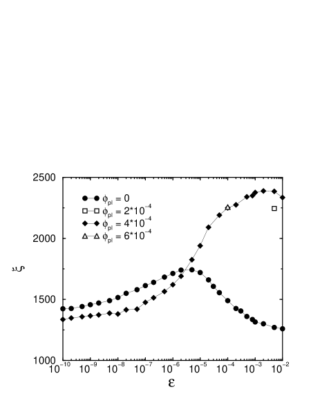
FIG. 6.: Localization length $\xi$ as functions of energy $\varepsilon$ for $\phi_{\rm pl}=0$, $2\times 10^{-4}$, $4\times 10^{-4}$, and $6\times 10^{-4}$ in the RRH model with $N=20$ chains. Averaging over $500$ realizations of disorder is performed.

In the presence of a magnetic field, $\xi$ increases by a factor $\sim 1.8$ in the crossover from the chiral-unitary to the standard unitary symmetry class, which is slightly less than the factor $2$ predicted in Eq. (76). Note that the increase in localization length is most rapid around the same energy scale $\varepsilon_{\rm c}\approx 5\times 10^{-6}$ for which $\xi$ reaches its maximum, $\xi_{\rm c}$, in the absence of a magnetic field. Moreover, $\varepsilon_{\rm c}$ is related to $\xi_{\rm c}$ by Thouless relation $\xi_{\rm c}\sim\sqrt{\ell/\varepsilon_{\rm c}}$ where the mean free path $\ell$ is obtained by dividing the localization length $\xi(\varepsilon=10^{-10})$ by $N=20$ in Fig. 6.

A plot of the ratio $C=-\lim_{L\to\infty}\langle\ln g\rangle/{\rm var}\ln g$ is shown in Fig. 7. In the standard symmetry classes, $C$ takes the universal value $C=1/2$, while in the chiral classes one has[43]

$$C = \frac{\beta N/2}{N+\left(1-\frac{2}{\pi}\right)(N-2+2\eta)}$$ (132)

$$= {\beta\over 4-4/\pi}+{\cal O}(1/N).$$ (133)

The data shown in Fig. 7 confirm that $C=0.5$ in the standard symmetry classes (corresponding to $\varepsilon\gtrsim 10^{-4}$ for the parameters of our simulation). However, for the chiral symmetry classes, a $20\%$ discrepancy with Eq. (133) is found.

While the numerical simulations for the localized regime qualitatively confirm the theory of Sec. IV, quantitative agreement is only up to $\sim 20\%$. As a possible source of this discrepancy, we point to the fact that the simulations are done for an appreciable disorder strength $\delta=0.2$, while the theory is derived for weak disorder, corresponding to $\delta\to 0$. Hence, the system cannot be considered truly (quasi) one-dimensional, and corrections from two-dimensional dynamics on shorter length scales need to be taken into account. Another cause of the observed discrepancies could be the uncertainty of the precise value of $\eta$ for the RRH model. While we believe that $\eta$ should not affect the conductance distribution significantly for large $N$, it remains difficult to make a quantitative assessment of finite-$N$ corrections as long as $\eta$ is unknown. At this moment, we are not aware of a direct way to obtain $\eta$ from the numerical simulations.

FIG. 7.: Ratio $C=-\lim_{L\to\infty}\langle\ln g\rangle/{\rm var}\ln g$ versus $\varepsilon$ for $\phi_{\rm pl}=0$ and $4\times 10^{-4}$ in the RRH model with $N=20$ chains and $L=4\times 10^{5}$. The disorder average is taken over $500$ realizations.

B Diffusive regime in the RRH and RF models

We next consider the crossover from the chiral symmetry classes to the standard symmetry classes in the diffusive regime $\ell\ll L\ll\xi$. In Figs. 8 and 9 we show numerical simulations of the average and variance of the conductance as a function of the energy $\varepsilon$ and the magnetic flux $\phi=L(N-1)\phi_{\rm pl}$ through the disordered part of the wire. The simulations are performed with $N=45$ and $L=800$, in order to ensure that the conditions $\ell\ll L\ll\xi$ for diffusive transport and $N\ll L$ for quasi-one-dimensionality are both met. The ensemble average is taken over $10^{4}$ samples.

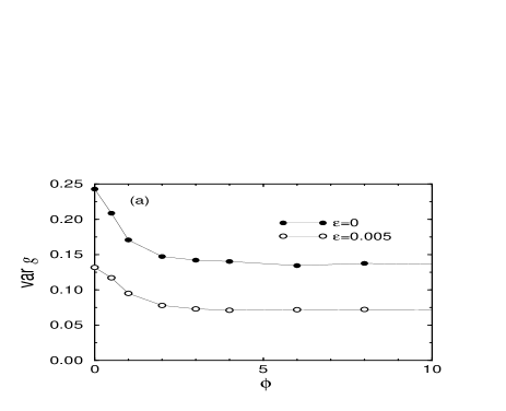
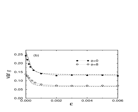
FIG. 8.: Variance of $g$ for the RRH model versus the total flux $\phi$ through the disordered wire (a) and versus energy $\varepsilon$ (b). In (a), $\mbox{var}\,g$ is shown for two values of the energy, $\varepsilon=0$ and $\varepsilon=0.005$, corresponding to the presence and absence of chiral symmetry; in (b), $\mbox{var}\,g$ is shown for two values of the flux $\phi=0$ and $\phi=8$, corresponding to the presence and absence of time-reversal symmetry. The dashed line in (b) is the theoretical curve (118), with $\sigma^{2}=1.5\times 10^{4}\varepsilon$. The simulations are performed for $N=45$, $L=800$, and an averaging over $10^{4}$ realizations of the disorder is performed.

Numerical results for the variance of the conductance in the RRH model versus $\phi$ and $\varepsilon$ are shown in Fig. 8. The numerical data of $\mbox{var}\,g$ versus $\phi$ (Fig. 8a) agree within $10\%$ with the theoretical predictions $\mbox{var}\,g=4/15$ ($2/15$) for $\phi=0$ and $\mbox{var}\,g=2/15$ ($1/15$) for $\phi\gg 1$ for $\varepsilon=0$ ($\varepsilon\gg 0$). The crossover between the orthogonal and unitary classes happens for $\phi\sim 1$, both with chiral symmetry ($\varepsilon=0$), and without ($\varepsilon=0.005$). The $\varepsilon$-dependence of $\mbox{var}\,g$ is shown in Fig. 8b, together with the theoretical result (118), where we fitted the crossover energy scale that enters into the definition of $\sigma=L/\ell_{\varepsilon}$, cf. Eq. (116). Again we find quantitative agreement well within $10\%$. (The fact that the numerical data for $\phi=0$ are below the theoretical curve can probably be attributed to the suppression of $\mbox{var}\,g$ as $L$ approaches the localization length $\xi$, see the remark in the discussion of Fig. 5.)

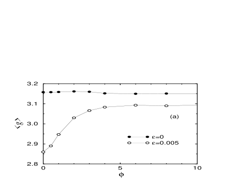
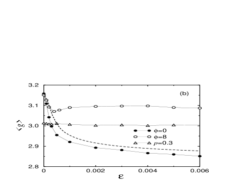
FIG. 9.: Mean conductance as a function of the total flux $\phi$ (a) and of the energy $\varepsilon$. In (a), data are shown for $\varepsilon=0$ and $\varepsilon=0.005$. In (b), $\langle g\rangle$ is shown for $\phi=0$ and $\phi=8$ for the RRH model (circles) and for the RF model at $p=0.3$ (triangles). All simulations were done for $N=45$ and $L=800$. The average was performed over $10^{4}$ realizations of the disorder. The dashed line in (b) is taken from Eq. (117) with $\beta=1$ and $\sigma^{2}=1.5\times 10^{4}\varepsilon$.

Numerical results for the average conductance are shown in Fig. 9. All data shown are for the same length $L=800$ and for the same number of channels $N=45$. For weak disorder one can ignore the $\phi$ and $\varepsilon$ dependence of the mean free path $\ell$, and hence of the Drude term in the conductance. The only effect of a variation of $\varepsilon$ or $\phi$ is thus to change the symmetry of the quantum wire, which affects the weak-localization correction to the conductance. According to Eq. (117), we expect a nonzero weak-localization correction $\delta g$ in the standard orthogonal symmetry class, i.e., for $\phi=0$ and $\varepsilon\neq 0$, while $\delta g=0$ if time-reversal symmetry is broken ($\phi\gtrsim 1$) or if the chiral symmetry is present ($\varepsilon=0$). This behavior is confirmed in Fig. 9. However, quantitatively, the numerical results differ $\sim 30\%$ from Eq. (117). In addition, Fig. 9 shows a small $\varepsilon$ dependence of $\langle g\rangle$ at large magnetic fields that cannot be accounted for within the theory of Sec. V. In particular, note the cusp-like structure at small $\varepsilon$ in the $\phi=8$ data in Fig. 9b. This effect seems to be too large to be explained by a spurious $\varepsilon$-dependence of the mean free path $\ell$. Since the feature at small $\varepsilon$ is suppressed at larger lengths $L$, a possible cause might be a contact resistance effect. (Contact resistance is known to play a role for disordered normal-metal–superconductor junctions, when the particle-hole degeneracy is destroyed by a finite voltage or by a magnetic field.[72]) As we discussed in the previous subsection, other causes for the discrepancy between theory and numerical simulations may be the fact that the disorder is not small, or that the parameter $\eta$ is not known.

VII Conclusions

In the vicinity of the band center, the physics of localization in a quantum wire with chiral symmetry exhibits differences with respect to the case of a quantum wire in one of the standard symmetry classes. The most prominent differences are observed in the localized regime. For wires with chiral symmetry (as is the case with off-diagonal disorder), at the band center, the statistics of the conductance depends sensitively on the parity in the number of transmission channels $N$. For odd $N$, the band center represents a critical point that is characterized by the absence of exponential localization. The logarithm of the conductance is not self-averaging and the mean conductance or its variance decay algebraically with the length $L$ of the wire. For even $N$, exponential localization takes place with a self-averaging localization length $\xi$ that does not depend on the presence or absence of time-reversal and spin rotation symmetry. As the energy is tuned away from the band center, the system crosses over to the standard universality classes: The parity effect disappears and the localization length acquires a dependence on the presence or absence of time-reversal and spin rotation symmetry. In the presence of time-reversal symmetry, the localization length $\xi$ for even $N$ is the same with and without chiral symmetry. Our numerical simulations indicate that the crossover is non-monotonous: in the crossover between the chiral and standard symmetry classes, $\xi$ differs from the values in the pure symmetry classes. A complete theoretical description of this crossover is still lacking.

In the diffusive regime, the differences between the chiral and standard universality classes are less pronounced. They show up in quantum interference corrections to the classical (Drude) conductance, which is the same in both cases. We have found that in the chiral classes, weak-localization corrections to the mean conductance $\langle g\rangle$ and, more generally, to the density of transmission eigenvalues vanish at the band center. This is the quasi-one-dimensional counterpart of a similar observation made by Gade and Wegner in their study of two-dimensional disordered systems with chiral symmetry.[23] The conductance fluctuations are twice as large at the band center relative to the standard universality classes, compatible with the presence of an extra symmetry in the system. We have calculated these quantum interference corrections as a function of energy, for the entire crossover from the chiral universality class at the band center $\varepsilon=0$ to the standard unitary classes for $\varepsilon$ far away from $0$. The theoretical predictions for this crossover agree qualitatively with numerical simulations though there remains sizable deviations between theory and numerics of the order of 10-30$\%$.

While the chiral symmetry classes have received an enormous amount of theoretical attention (see the introduction of this paper for a brief summary), there are several hurdles to take before a chiral quantum wire can be realized in practice. Besides the effect of electron-electron interactions, which is not taken into account here, the main obstacle is the fact that the chiral symmetry is very fragile, since it is easily broken by, e.g., on-site random energies, next-nearest-neighbor hopping, or a small shift of the chemical potential, which will drive the system away from the chiral symmetric band center. Our calculation of the quantum interference corrections in the crossover from the chiral symmetry classes to the standard ones can be seen as a first and necessary step to tackle the latter obstacle.

A Scaling equations

In this appendix, we present the scaling equations needed to calculate the crossover for the weak localization corrections of the conductance, shot noise, and the universal conductance fluctuations of the conductance as done in Sec. V C. The notation was defined in Eq. (89) and we use the short-hands

$$R\equiv R_{10},\qquad R_{2}\equiv R_{1010},\qquad R_{3}\equiv R_{101010}.$$

Equations needed up to corrections of order $N^{0}$ are

$${\gamma\ell\over\beta}\partial_{L}\left\langle R\right\rangle =N\left\langle N-2R\right\rangle+\left\langle R\right\rangle^{2}+{2-\beta\over\beta}\left\langle N-R^{\ }_{00}-2R-R^{*}_{00}+R^{\ }_{1000}+R^{*}_{1000}+R^{\ }_{2}\right\rangle,$$ (A1)

$${\gamma\ell\over\beta}\partial_{L}\left\langle R^{\ }_{2}\right\rangle =4\left\langle R-R^{\ }_{2}\right\rangle\left(N-\left\langle R\right\rangle\right)$$ (A4)

$$+{2-\beta\over\beta}\left\langle R^{\ }_{00}+4R+R^{*}_{00}-8R^{\ }_{2}-4R^{\ }_{1000}-4R^{*}_{1000}+4R^{\ }_{3}+2R^{\ }_{101000}+2R^{*}_{101000}+R^{\ }_{100100}+R^{*}_{100100}\right\rangle,$$

$${\gamma\ell\over\beta}\partial_{L}{\rm var}\,R =4\left(\left\langle R\right\rangle-N\right){\rm var}\,R+\left\langle R^{\ }_{00}+R^{*}_{00}+2R-2R^{\ }_{1000}-2R^{*}_{1000}-4R^{\ }_{2}+R^{\ }_{100100}+R^{*}_{100100}+2R^{\ }_{3}\right\rangle$$ (A7)

$$+{2-\beta\over\beta}\left\langle R^{\ }_{00}+R^{*}_{00}+2R-2R^{\ }_{1000}-2R^{*}_{1000}-4R^{\ }_{2}+R^{\ }_{100100}+R^{*}_{100100}+2R^{\ }_{3}\right\rangle.$$

Equations needed up to corrections of order $N$ are

$${\gamma\ell\over\beta}\partial_{L}\left\langle R^{\ }_{00}\right\rangle ={4{i}\varepsilon\gamma\ell\over\beta}\left\langle R^{\ }_{00}\right\rangle+N\left\langle N-2R^{\ }_{00}\right\rangle+\left\langle R^{\ }_{00}\right\rangle^{2},$$ (A8)

$${\gamma\ell\over\beta}\partial_{L}\left\langle R^{\ }_{1000}\right\rangle ={4{i}\varepsilon\gamma\ell\over\beta}\left\langle R^{\ }_{1000}\right\rangle+N\left\langle 2R^{\ }_{00}+2R-4R^{\ }_{1000}\right\rangle-\left\langle R^{\ }_{00}+2R-2R^{\ }_{1000}\right\rangle\left\langle R^{\ }_{00}\right\rangle-\left\langle R-2R^{\ }_{1000}\right\rangle\left\langle R\right\rangle,$$ (A10)

$${\gamma\ell\over\beta}\partial_{L}\left\langle R^{\ }_{1100}\right\rangle =N\left\langle R^{\ }_{00}+2R+R^{*}_{00}-4R^{\ }_{1100}\right\rangle-\left\langle 2R-R^{\ }_{1100}\right\rangle\left\langle R^{\ }_{00}\right\rangle-\left\langle 2R^{*}_{00}-2R^{\ }_{1100}\right\rangle\left\langle R\right\rangle+\left\langle R^{\ }_{1100}\right\rangle\left\langle R^{*}_{00}\right\rangle,$$ (A12)

$${\gamma\ell\over\beta}\partial_{L}\left\langle R^{\ }_{3}\right\rangle =3\left(2N\left\langle R^{\ }_{2}-R^{\ }_{3}\right\rangle+\left\langle R-4R^{\ }_{2}+2R^{\ }_{3}\right\rangle\left\langle R\right\rangle+\left\langle R^{\ }_{2}\right\rangle^{2}\right),$$ (A14)

$${\gamma\ell\over\beta}\partial_{L}\left\langle R^{\ }_{101000}\right\rangle ={4{i}\varepsilon\gamma\ell\over\beta}\left\langle R^{\ }_{101000}\right\rangle+2\left(N\left\langle 2R^{\ }_{1000}+R^{\ }_{2}-3R^{\ }_{101000}\right\rangle+\left\langle R-R^{\ }_{1000}-R^{\ }_{2}+R^{\ }_{101000}\right\rangle\left\langle R^{\ }_{00}\right\rangle\right)$$ (A17)

$$+\left\langle R-6R^{\ }_{1000}-2R^{\ }_{2}+4R^{\ }_{101000}\right\rangle\left\langle R\right\rangle+\left\langle R^{\ }_{1000}+2R^{\ }_{2}\right\rangle\left\langle R^{\ }_{1000}\right\rangle,$$

$${\gamma\ell\over\beta}\partial_{L}\left\langle R^{\ }_{100100}\right\rangle ={4{i}\varepsilon\gamma\ell\over\beta}\left\langle R^{\ }_{100100}\right\rangle+2N\left\langle 2R^{\ }_{1000}+R^{\ }_{1100}-3R^{\ }_{100100}\right\rangle+\left\langle R^{\ }_{00}-4R^{\ }_{1000}+2R^{\ }_{100100}\right\rangle\left\langle R^{\ }_{00}\right\rangle$$ (A20)

$$+2\left\langle R-2R^{\ }_{1000}-2R^{\ }_{1100}+2R^{\ }_{100100}\right\rangle\left\langle R\right\rangle+2\left\langle R^{\ }_{1000}\right\rangle^{2}+\left\langle R^{\ }_{1100}\right\rangle^{2}.$$

REFERENCES

- [1] Present address: Paul Scherrer Institut, CH-5232, Villigen PSI, Switzerland.
- [2] Present address: Laboratory of Atomic and Solid State Physics, Cornell University, Ithaca, New York 14853-2501.
- [3] J. T. Edwards, and D. J. Thouless, J. Phys. C 5, 807 (1972); D. C. Licciardello, and D. J. Thouless, J. Phys. C 8, 4157 (1975); 11, 925 (1978); F. J. Wegner, Z. Phys. B 25, 327 (1976); E. Abrahams, P. W. Anderson, D. C. Licciardello, and T. V. Ramakrishnan, Phys. Rev. Lett. 42, 673 (1979).
- [4] For a review, see P. A. Lee and T. V. Ramakrishnan, Rev. Mod. Phys. 57, 287 (1985).
- [5] P. W. Anderson, E. Abrahams, and T. V. Ramakrishnan, Phys. Rev. Lett. 43, 718 (1979).
- [6] L. P. Gor’kov, A. I. Larkin, and D. E. Khmel’nitskiǐ, Pis’ma Zh. Eksp. Teor. Fiz. 30, 248 (1979) [JETP Lett. 30, 228 (1979)].
- [7] B. L. Al’tshuler, Pis’ma Zh. Eksp. Teor. Fiz. 41, 530 (1985) [JETP Lett. 41, 648].
- [8] P. A. Lee and A. D. Stone, Phys. Rev. Lett. 55, 1622 (1985).
- [9] For a review, see Y. Imry, in Mesoscopic Quantum Physics, edited by E. Akkermans, G. Montambaux, J.-L. Pichard, and J. Zinn-Justin (North-Holland, Amsterdam, 1995).
- [10] P. W. Anderson, Phys. Rev. 109, 1492 (1958).
- [11] D. C. Herbert and R. Jones, J. Phys. C: Solid St. Phys. 4, 1145 (1971).
- [12] F. J. Dyson, Phys. Rev. 92, 1331 (1953).
- [13] I. M. Lifschitz, Usp. Fiz. Nauk 83, 617 (1964) [Sov. Phys. Usp. 7, 549 (1965)].
- [14] L. V. Keldysh, Zh. Eksp. Teor. Fiiz. 45, 364 (1963) [Sov. Phys. JETP 18, 253 (1964)].
- [15] G. Theodorou and M. H. Cohen, Phys. Rev. B 13, 4597 (1976).
- [16] L. Fleishman and D. C. Licciardello, J. Phys. C 10, L125 (1977).
- [17] T. P. Eggarter and R. Riedinger, Phys. Rev. B 18, 569 (1978).
- [18] R. Oppermann and F. Wegner, Z. Phys. B 34, 327 (1979).
- [19] F. Wegner, Z. Phys. B 44, 9 (1981).
- [20] A. D. Stone and J. D. Joannopoulos, Phys. Rev. B 24, 3592 (1981).
- [21] D. J. Thouless, J. Phys. C 5, 77 (1972).
- [22] H. Mathur, Phys. Rev. B 56, 15 794 (1997).
- [23] R. Gade, Nucl. Phys. B 398, 499 (1993); R. Gade and F. Wegner, ibid. 360, 213 (1991); F. J. Wegner, Phys. Rev. B 19, 783 (1979);
- [24] S. Hikami, M. Shirai, and F. Wegner, Nucl. Phys. B 408, 413 (1993); K. Minakuchi and S. Hikami, Phys. Rev. B 53, 10 898 (1996).
- [25] T. Fukui, Nucl. Phys. B 562, 477 (1999).
- [26] A. Altland and B. D. Simons, Nucl. Phys. B 562, 445 (1999).
- [27] M. Fabrizio and C. Castellani, cond-mat/0002328.
- [28] See A. Furusaki, Phys. Rev. Lett. 82, 604 (1999) and references therein.
- [29] See, e.g., B. Huckestein, Rev. Mod. Phys. 67, 357 (1995).
- [30] T. A. L. Ziman, Phys. Rev. B 26, 7066 (1982).
- [31] M. Inui, S. A. Trugman, and E. Abrahams, Phys. Rev. B 49, 3190 (1994).
- [32] C. Mudry, P. W. Brouwer, and A. Furusaki, Phys. Rev. B 59, 13221 (1999).
- [33] For a review, see T. Guhr, A. Mueller-Groeling, and H. A. Weidenmueller, Phys. Rep. 299, 190 (1998).
- [34] J. J. M. Verbaarschot and I. Zahed, Phys. Rev. Lett. 70, 3852 (1993).
- [35] B. M. McCoy and T. T. Wu, Phys. Rev. 176, 631 (1968); E. R. Smith, J. Phys. C 3, 1419 (1970); R. Shankar and G. Murthy, Phys. Rev. B 36, 536 (1987); D. S. Fisher. Phys. Rev. B 50, 3799 (1994); 51, 6411 (1995); R. H. McKenzie, Phys. Rev. Lett. 77, 4804 (1996).
- [36] J. Miller and J. Wang, Phys. Rev. Lett. 76, 1461 (1996). For reviews, see J-P. Bouchaud, and A. Georges, Phys. Rep. 195, 127 (1990); M. B. Isichenko, Rev. Mod. Phys. 64, 961 (1992).
- [37] For a review, see A. Comtet and C. Texier, in “Supersymmetry and Integrable Models”, edited by H. Aratyn, T. D. Imbo, W-Y. Keung, U. Sukhatme, (Springer-Verlag, Berlin 1999).
- [38] H-J. Sommers, A. Crisanti, H. Sompolinsky, and Y. Stein, Phys. Rev. Lett. 60, 1895 (1988); Y. V. Fyodorov, B. A. Khoruzhenko, and H-J. Sommers, Phys. Lett. A 226, 46 (1997); C. Mudry, B. D. Simons, and A. Altland, Phys. Rev. Lett. 80, 4257 (1998).
- [39] A. W. W. Ludwig, M. P. A. Fisher, R. Shankar, and G. Grinstein, Phys. Rev. B 50, 7526 (1994); A. A. Nersesyan, A. M. Tsvelik, and F. Wenger, Phys. Rev. Lett. 72, 2628 (1994); C. Mudry, C. Chamon, and X.-G. Wen, Nucl. Phys. B 466, 383 (1996); H. E. Castillo, C. de C. Chamon, E. Fradkin, P. M. Goldbart, and C. Mudry, Phys. Rev. B 56, 10 668 (1997); Y. Hatsugai, X.-G. Wen, and M. Kohmoto, Phys. Rev. B 56, 1061 (1997); Y. Morita and Y. Hatsugai, Phys. Rev. Lett. 79, 3728 (1997); Phys. Rev. B 58, 6680 (1998);
- [40] A. Eilmes, R. A. Römer, and M. Schreiber, Eur. Phys. J. B 1, 29 (1998); P. Biswas, P. Cain, R. A. Römer, and M. Schreiber, cond-mat/0001315.
- [41] A. MacKinnon and B. Kramer, Z. Phys. B 53, 1 (1983).
- [42] P. W. Brouwer, C. Mudry, B. D. Simons, and A. Altland, Phys. Rev. Lett. 81, 862 (1998).
- [43] P. W. Brouwer, C. Mudry, and A. Furusaki, Nucl. Phys. B 565, 653 (2000).
- [44] For a review, see C. W. J. Beenakker, Rev. Mod. Phys. 69, 731 (1997).
- [45] O. N. Dorokhov, Pis’ma Zh. Eksp. Teor. Fiz. 36, 259 (1982) [JETP Lett. 36, 318 (1982)].
- [46] P. A. Mello, P. Pereyra, and N. Kumar, Ann. Phys. (N.Y.) 181, 290 (1988).
- [47] F. D. M. Haldane, Phys. Lett. 93A, 464 (1983); Phys. Rev. Lett. 50, 1153 (1983).
- [48] For a review, see E. Dagotto and T. M. Rice, Science 271, 618 (1996).
- [49] P. W. Brouwer, C. Mudry, and A. Furusaki, Phys. Rev. Lett. 84, 2913 (2000).
- [50] P. W. Brouwer, Phys. Rev. B 57, 10526 (1998).
- [51] See section of M. L. Mehta, Random matrices (Academic Press, London, 1991).
- [52] M. Büttiker, Phys. Rev. Lett. 65, 2901 (1990); For reviews, see Th. Martin, in Coulomb and Interferences Effects in Small Electronic Structures, edited by D. C. Glatti, M. Sanquer, and J. Trân Vân (Editions Frontières, Gif-sur-Yvette, France), and M. J. M. De Jong and C. W. J. Beenakker, in Mesoscopic Electron Transport, edited by L. P. Kouwenhoven, G. Schön, and L. L. Sohn, NATO ASI Series E (Kluwer, Dordrecht, 1998); Ya. M. Blanter and M. Büttiker, cond-mat/9910158.
- [53] P. W. Anderson, D. J. Thouless, E. Abrahams, and D. S. Fisher, Phys. Rev. B 22, 3519 (1980).
- [54] M. R. Zirnbauer, Phys. Rev. Lett. 69, 1584 (1992).
- [55] C. W. J. Beenakker and B. Rejaei, Phys. Rev. Lett. 71, 3689 (1993); Phys. Rev. B 49, 7499 (1994).
- [56] A. D. Mirlin A. Müller-Groeling, and M. R. Zirnbauer, Ann. Phys. (N.Y.) 236, 325 (1994).
- [57] K. Frahm, Phys. Rev. Lett. 74, 4706 (1995).
- [58] P. W. Brouwer and K. Frahm, Phys. Rev. B 53, 1490 (1996).
- [59] O. N. Dorokhov, Zh. Eksp. Teor. Fiz. 85, 1040 (1983) [Sov. Phys. JETP 58, 606 (1983)].
- [60] J.-L. Pichard, in Quantum Coherence in Mesoscopic Systems, edited by B. Kramer, NATO ASI Series B254 (Plenum, New York), p. 369 (1991).
- [61] P. A. Mello, and A. D. Stone, Phys. Rev. B 44, 3559 (1991).
- [62] T. Ohtsuki, K. Slevin, and Y. Ono, J. Phys. Soc. Jpn. 62, 3979 (1993).
- [63] P. W. Brouwer and C. W. J. Beenakker, Phys. Rev. B 52, 16772 (1995).
- [64] H. U. Baranger and P. A. Mello, Phys. Rev. B 54, 14297 (1996).
- [65] O. N. Dorokhov, Solid State Commun. 51, 381 (1984).
- [66] P. A. Mello and J.-L. Pichard, Phys. Rev. B 40, 5276 (1989).
- [67] L. Balents and M. P. A. Fisher, Phys. Rev. B 56, 12 970 (1997).
- [68] These are the limiting values for weak disorder, , the wave length at the Fermi energy. For strong disorder, averages like may also be nonzero for models with on-site disorder, see e.g. V. Freilikher and M. Pustilnik, Phys. Rev. B 55, 653 (1997).
- [69] T. Ando, Phys. Rev. B 40, 5325 (1989).
- [70] H. U. Baranger, D. P. DiVincenzo, R. A. Jalabert, and A. D. Stone, Phys. Rev. B 44, 10637 (1991).
- [71] Yu. V. Nazarov and T. H. Stoof, Phys. Rev. Lett. 76, 823 (1996).
- [72] P. W. Brouwer and C. W. J. Beenakker, Phys. Rev. B 52, R3836 (1995).