A new approach to the study of the ground-state
properties of 2D Ising spin glass

A new approach known as flat histogram method is used to study the $\pm J$ Ising spin glass in two dimensions. Temperature dependence of the energy, the entropy, and other physical quantities can be easily calculated and we give the results for the zero-temperature limit. For the ground-state energy and entropy of an infinite system size, we estimate $e^{0}=-1.4007\pm 0.0085$ and $s^{0}=0.0709\pm 0.006$, respectively. Both of them agree well with previous calculations. The time to find the ground-states as well as the tunneling times of the algorithm are also reported and compared with other methods.

Key words: Monte Carlo dynamics; Flat histogram sampling; Ising spin glass; Ground-states; Tunneling time.

PACS numbers: 02.70.Lq, 05.50+q, 05.10.Ln, 75.10.Nr, 75.40.Mg.

1 Introduction

The equilibrium properties of spin glass have remained a great challenge in numerical simulations. Investigating the equilibrium ground-state structure of spin glass is also important and interesting. In the last 20 years, there has been a great deal of work on spin glass [1]. It is generally agreed that the simplest spin glass system for most theoretical work is the Edwards-Anderson (EA) model, whose Hamiltonian is

$$H=-\sum_{<i,j>}J_{ij}\sigma_{i}\sigma_{j},$$ (1)

where $\sigma_{i}$ takes on the values $\pm 1$ and the sum goes over the nearest neighbors. The $J_{ij}$ are dimensionless variables which describe the random interactions between the spins and are taken as $J_{ij}=\pm 1$. In two dimensions, a phase transition occurs only at zero temperature [2, 3, 4] for this kind of $\pm J$ Ising spin glass with nearest neighbor interactions. This model has been studied previously by the transfer matrix method [2, 5], replica Monte Carlo method [4, 6], multicanonical ensemble method [7] and many other methods (see ref [1] for a review).

The traditional Monte Carlo methods mostly concentrate on generating standard statistical ensembles, e.g., the canonical ensemble or microcanonical ensemble. Using the canonical ensemble simulations, we need to simulate at different temperatures to get full information about the system. It is tedious to calculate certain thermodynamic quantities like the free energy and the entropy since the density of states cannot be obtained directly from the simulation data. The correlation between subsequent configurations generated by canonical ensemble simulations also causes the ergodicity problem for some systems. In 1991, Berg proposed the multicanonical ensemble method [8] to overcome the above shortcomings of simulations on canonical ensemble. The multicanonical ensemble is an ensemble where the probability $P(E)$ of having energy $E$ at equilibrium is a constant. The multicanonical method has been very successful in solving the systems that involve energy barriers.

Recently, Wang proposed a dynamics [9] which can generate a flat histogram in the energy space as the multicanonical method. This dynamics has some connections with the broad histogram method [10], which does not give the correct microcanonical average [9]. Similar to the broad histogram method, the new dynamics is also based on $\langle N(\sigma,\Delta E)\rangle$, the (microcanonical) average number of potential moves which increase the energy by $\Delta E$ in a single spin flip. A cumulative average (over Monte Carlo steps) can be used as a first approximation to the exact microcanonical average in the flip rate. Thermodynamic quantities can be then calculated from the simulation data with ease. In this paper, we use the new method to study the thermodynamics as well as ground-state properties for the two-dimensional Ising spin glass system.

In Section 2, the flat histogram transition matrix Monte Carlo dynamics is described. Using the flat histogram sampling, we get the average number of potential moves $\langle N(\sigma,\Delta E)\rangle_{E}$, which can be used to construct a transition matrix Monte Carlo dynamics in the energy space [11]. We apply the new method to two-dimensional Ising spin glass and present some numerical results in Section 3. In the last section, we give a conclusion to the new method.

2 The transition matrix Monte Carlo dynamics with the flat histogram sampling

To connect our dynamics with single-spin-flip Glauber dynamics [12], we restrict the protocol of each move to be single-spin flip in the following discussion. For a given state $\sigma$ with energy $E$, consider all possible single-spin flips. The single-spin flips change the current state into $N$ possible new states, with new energy $E^{\prime}=E+\Delta E$. For two-dimensional Ising spin glass, $\Delta E$ = $0$, $\pm 4$, and $\pm 8$. We classify the $N$ new states according to $\Delta E$ and count the number of $N(\sigma,\Delta E)$. Since each move from the state $\sigma$ of energy $E$ to the state $\sigma^{\prime}$ of energy $E^{\prime}$ and the reverse move are both allowed, the total number of moves from all the states with energy $E$ to $E^{\prime}$ is the same as from $E^{\prime}$ to $E$. Thus, we have [13]

$$\sum_{E(\sigma)=E}N(\sigma,\Delta E)=\sum_{E(\sigma^{\prime})=E+\Delta E}N(\sigma^{\prime},-\Delta E).$$ (2)

The microcanonical average of a quantity $A(\sigma)$ is defined as

$$\langle A\rangle_{E}=\frac{1}{n(E)}\sum_{E(\sigma)=E}A(\sigma),$$ (3)

where the summation is over all the configurations having energy $E$ and $n(E)$ is the density of states. In terms of the microcanonical averages, we can rewrite Eq. (2) as

$$n(E)\langle N(\sigma,\Delta E)\rangle_{E}=n(E+\Delta E)\langle N(\sigma^{\prime},-\Delta E)\rangle_{E+\Delta E}.$$ (4)

Eq. (4) is the basic result of the broad histogram method [10]. While the broad histogram random walk algorithm is not correct, Eq. (4) is not problematic and taken as the starting point of the flat histogram sampling.

We select a site to flip at random. The flip rate for a single-spin flip from state $\sigma$ with energy $E$ to $\sigma^{\prime}$ with energy $E^{\prime}=E+\Delta E$ is chosen as

$$r(E^{\prime}|E)=\min\Big{(}1,\frac{\langle N(\sigma^{\prime},-\Delta E)\rangle_{E^{\prime}}}{\langle N(\sigma,\Delta E)\rangle_{E}}\Big{)}.$$ (5)

Then the detailed balance condition for this rate

$$r(E^{\prime}|E)P(\sigma)=r(E|E^{\prime})P(\sigma^{\prime})$$ (6)

is satisfied for $P(\sigma)\propto 1/n(E(\sigma))$. Thus the energy histogram is flat [13],

$$P(E)=\sum_{E(\sigma)=E}P(\sigma)\propto n(E)\frac{1}{n(E)}=\textnormal{const}.$$ (7)

Since $\langle N(\sigma,\Delta E)\rangle_{E}$ is not known in general, an approximation scheme should be used to start the simulation. For those $E$ which we have not visited yet, we simply set $r(E^{\prime}|E)=1$. Then a cumulative average (over Monte Carlo steps) can be used as an approximation to the exact microcanonical average in the flip rate. We have numerical evidence that this procedure converges to the exact result.

We can then construct a transition matrix Monte Carlo dynamics in the energy space [11] with $\langle N(\sigma,\Delta E)\rangle_{E}$. For a single-spin-flip Glauber dynamics with energy change $\Delta E$, the flip rate is given as

$$w(\Delta E)=\frac{1}{2}\Big{[}1-\tanh\Big{(}\frac{\Delta E}{2k_{B}T}\Big{)}\Big{]}.$$ (8)

Since there are (on average) $\langle N(\sigma,\Delta E)\rangle_{E}$ different ways of going from $E$ to $E^{\prime}=E+\Delta E$, the total probability for transition from $E$ to $E^{\prime}$ is

$$W(E+\Delta E|E)=w(\Delta E)\langle N(\sigma,\Delta E)\rangle_{E},\qquad for~{}\Delta E\neq 0.$$ (9)

The diagonal elements can be determined by $\sum_{\Delta E}W(E+\Delta E|E)=1$, since the total probability from $E$ to $E^{\prime}$ is 1. This new dynamics in the space of energy $E$ is related to single-spin-flip dynamics by [11]

$$W(E^{\prime}|E)=\frac{1}{n(E)}\sum_{E(\sigma)=E}\sum_{E(\sigma^{\prime})=E^{\prime}}\Gamma(\sigma^{\prime}|\sigma).$$ (10)

where $\Gamma(\sigma^{\prime}|\sigma)$ is the transition matrix of the single-spin-flip dynamics. The equilibrium state of the transition matrix gives the canonical probability distribution of energy $P_{T}(E)\propto n(E)\exp(-E/k_{B}T)$.

An important aspect of this dynamics is that we can calculate the thermodynamic quantities easily by just performing one simulation for each coupling state $J_{ij}$. The density of states $n(E)$ can be obtained through Eq. (4). Once we have the density of states $n(E)$, we can obtain $P_{T}(E)$ and then calculate any thermodynamic quantities of interest. In actual implementation, we usually determine $P_{T}(E)$ directly from the detailed balance equation

$$W(E+\Delta E|E)P_{T}(E)=W(E|E+\Delta E)P_{T}(E+\Delta E)$$ (11)

instead of solving Eq. (4). From Eq. (9), we know, the transition matrix $W(E^{\prime}|E)$ can be formed at any temperature once the quantity $\langle N(\sigma,\Delta E)\rangle_{E}$ is computed accurately. In other words, the Monte Carlo computation is uncorrelated to thermodynamics. The temperature dependence enters only after simulation in the weighting formula.

Like Berg’s multicanonical ensemble simulations, our dynamics also generate a multicanonical ensemble in the energy space. From this point, both of the two dynamics have the same goal of flattening the space of energy. But they are quite different in implementation. In the multicanonical ensemble method, the flip rate is chosen as the inverse of the density of states $n(E)$, parametrized in some way. To start the simulation, we need give an estimate of $n(E)$, since $n(E)$ is not initially known. Thus, the efficiency of this method is determined by the goodness of the estimated $n(E)$. If $n(E)$ is not given properly, say far off the true density, the simulations may get stuck in some region. With our method, we sample the energy space with a flip rate which is related to the density of states through Eq. (4). The central quantity is $\langle N(\sigma,\Delta E)\rangle_{E}$ which can be quite accurate in a short simulation time. And the accuracy of this quantity is improved by further simulations. We then provide an alternate for the estimate of $n(E)$, which leads to a more efficient way for simulating the multicanonical ensemble.

The flat histogram also generalizes easily to multi-variate models [14]. An example is the Ising Spin Glass model with overlap parameter $q$ which has the Hamiltonian

$$H_{2}=-\sum_{<i,j>}J_{ij}\sigma_{i}^{1}\sigma_{j}^{1}-\sum_{<i,j>}J_{ij}\sigma_{i}^{2}\sigma_{j}^{2}-h\underbrace{\sum_{i}\sigma_{i}^{1}\sigma_{i}^{2}}_{q}.$$ (12)

$E$ refers to the first two interaction terms involving the coupling constants $J_{ij}$. In this bivariate case, the quantity $\langle N(\sigma,\Delta E)\rangle$ generalize to $\langle N(\sigma,\Delta E,\Delta q)\rangle$. It can be easily shown that the detailed balance condition is now

$$n(E,q)\langle N(\sigma,\Delta E,\Delta q)\rangle_{E,q}=n(E+\Delta E,q+\Delta q)\langle N(\sigma^{\prime},-\Delta E,-\Delta q)\rangle_{E+\Delta E,q+\Delta q}$$ (13)

with $n(E,q)$ as the new “density of states”. The algorithm gives a flat histogram in both $E$ and $q$.

3 Numerical results

We have performed simulations on lattices of size $L=4,10,16,24$ and $32$. Each simulation starts with independent random numbers. To illustrate the performance of our algorithm, we define the time $\tau_{L}$ as the average number (over coupling constant $J_{ij}$) of Monte Carlo steps needed to reach the ground-states. A Monte Carlo step is defined as flipping each spin on the lattice once (on the average). Table 1 gives an overview of typical time in Monte Carlo steps to reach the ground-states, starting from an arbitrary energy level. The time to reach the ground-states depends on the size of the system and also the random interactions. We consider a large number of random coupling states to make the statistical error small enough in Table 1. The simulations are long enough to ensure that the ground states are really reached. In Fig.1 we plot the time $\tau_{L}$ versus lattice size $L$ on a double log scale. The data are consistent with a straight-line fit, which gives the finite-size behavior

$$\tau_{L}\propto L^{4.71},\quad\textnormal{MC~{}steps}.$$ (14)

The corresponding CPU time for a Digital Alpha 600M workstation is also shown in Table 1. For accuracy, 5 independent runs are performed for each lattice size to obtain the average CPU time. Up to $L=32$ the CPU time can be approximated by a polynomial function of $L^{6.08}$.

L	$\tau_{L}$(MC Steps)	CPU time(second)
4	45.33 $\pm$ 0.91	0.003 $\pm$ 0.001
10	2752 $\pm$ 127	0.43 $\pm$ 0.012
16	25761 $\pm$ 1504	8.55 $\pm$ 0.55
24	216884 $\pm$ 18444	189 $\pm$ 15
32	759609 $\pm$ 80310	733 $\pm$ 86

Table 1: Average MC steps and CPU time to find the ground-states for different lattice size.

We also consider the tunneling time which is defined as the average Monte Carlo steps needed to move from $E_{max}$ to $E_{min}$, or from $E_{min}$ to $E_{max}$. Note that $E_{min}$ is the same as ground state energy and $E_{max}$ is $N-E_{min}$. We note that Berg’s definition about tunneling time is slightly different from ours. During the simulation, Berg imposed a constraint $\sum_{ij}J_{ij}=0$. But for our method, both the time $\tau_{L}$ and the tunneling time will not be affected significantly by the imposition of the constraint. We start the simulations from an arbitrary energy level. Table 2 gives an overview of the tunneling time obtained using the two methods. The power law fits are

$$\tau_{M.C.}\propto L^{4.43},\;\;\;\textnormal{and}\;\;\;\tau_{F.H.}\propto L^{5.03},$$ (15)

for Berg’s method and current flat histogram method, respectively. It shows that they basically give the same tunneling time.

$L$	Flat Histogram (F.H.)	Multicanonical (M.C.)	Bivariate in $q$ ($q$)
4	27.4 $\pm$ 0.14	35.3 $\pm$ 2.8	75.1 $\pm$ 3.0
8	541 $\pm$ 9		($1.82\pm 0.23)\times 10^{3}$
12	$(4.71\pm 0.3)\times 10^{3}$	$(2.61\pm 0.45)\times 10^{3}$	($9.68\pm 1.08)\times 10^{3}$
16			($3.74\pm 0.31)\times 10^{4}$
24	$(2.22\pm 0.6)\times 10^{5}$	$(1.94\pm 0.44)\times 10^{5}$
48		$(1.46\pm 0.52)\times 10^{6}$

Table 2: Average tunneling time obtained with two dynamics for different lattice sizes. The multicanonical results are obtained from Ref. [7].

We also compared with Hatano’s result [15] that autocorrelation time scales approximately as volume $N$ of the system. We look at the tunneling time which is a better measure of the algorithm’s efficiency in our case. From our results given in Table 2, we found no support for Hatano’s result. Instead, the power law fit (see Fig. 2)

$$\tau_{q}\propto L^{4.45}$$ (16)

is almost the same as the monovariate case. This is not surprising as Berg mentioned that the optimal performance for multicanonical algorithm is $\propto N$(=$L^{2}$) based on random walk picture.

The ground-state energy and entropy of the infinite system are also estimated using our method. It is straightforward to obtain the ground-state energy in the simulation stage. We calculate the ground-state entropy from

$$S(E)=\frac{k_{B}}{N}\ln n(E).$$ (17)

Since $n(E)$ can be calculated from the simulation data directly, we then obtain $S(E)$ with ease.

To compare with the results obtained in the literature, we fit our data using the form $f_{L}=f_{\infty}+c/L^{2}$ and get $e^{0}=-1.4007\pm 0.0085$, $s^{0}=0.0709\pm 0.006$. The energy fit is plotted in Fig. 3, and the entropy fit in Fig. 4. Our energy estimate $e^{0}=-1.4007\pm 0.0085$ is consistent with the previous MC estimate [4] $e^{0}=-1.407\pm 0.008$ as well as with the transfer matrix result [5] $e^{0}=-1.4024\pm 0.0012$. Our entropy estimate $s^{0}=0.0709\pm 0.006$ is also consistent with the MC estimate [4] $s^{0}=0.071\pm 0.007$ as well as the transfer matrix result [5] $s^{0}=0.0701\pm 0.005$. For the two-dimensional Ising spin glass system, De Simone et al. [16] use an exact algorithm based on the branch-and-cut technique to find the exact ground-states with system size up to $50\times 50$. They obtain the extrapolated result $e^{0}=-1.4022\pm 0.0003$. When compared with Berg’s result, $e^{0}=-1.394\pm 0.007,s^{0}=0.081\pm 0.004$, it seems that our method gives a more accurate estimate for ground-state energy and entropy for an infinite system.

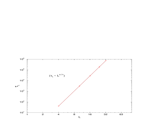
Figure 1: $\tau_{L}$ vs lattice size on a double log scale.

Figure 2: Tunneling time of bivariate model on a double log scale.

Figure 3: FSS estimate of energy per spin of the infinite system size.

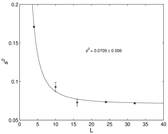
Figure 4: FSS estimate of entropy per spin of the infinite system size.

4 Conclusions

We have used a new approach to investigate the ground-state properties of the two-dimensional Ising spin glass. Compared with standard simulations, the advantage of our method is obvious. For the ergodicity problem encountered in standard simulations, our method behaves as well as Berg’s multicanonical ensemble method, while it is easier to be implemented compared with Berg’s method. Our method also generalize straightforwardly to multi-variate models without much effort in programming and theory.

To find a true ground-state, we roughly need a CPU time of order $L^{6}$. It is the same with Lawler’s exact algorithm [17]. Up to size $50\times 50$, De Simone’s algorithm also needs a time of order $L^{6}$. But it is not clear whether his algorithm can be efficiently implemented for 3D systems. However our method can also be easily applied to 3D spin glass system. If one is just interested in finding the ground-states, there are also other optimized algorithms. Chen’s learning algorithm [18] is fast in finding the ground-states compared with most algorithms, but it is not a general one. Thermodynamic quantities cannot be obtained with this algorithm.

We believe that the approach we present in this paper is useful in studying the thermodynamics as well as ground-state properties for spin glass systems. It also can be applied to other models because of its generality.

References

- [1] K.Binder and A. P. Young, Rev. Mod. Phys. 58, 801 (1986).
- [2] I. Morgenstern and K. Binder, Phys. Rev. Lett. 43, 1615 (1979); Phys. Rev. B 22, 288 (1980).
- [3] W. L. McMillan, Phys. Rev. B 28, 5216 (1983).
- [4] R. H. Swendsen and J.-S. Wang, Phys. Rev. Lett. 57, 2607 (1986).
- [5] H.-F. Cheung and W. L. McMillan, J. Phys. C 16, 7027 (1983).
- [6] J.-S. Wang and R. H. Swendsen, Phys. Rev. B 38, 4840 (1988).
- [7] B. Berg and T. Celik, Phys. Rev. Lett. 69 2292 (1992).
- [8] B. Berg and T. Neuhaus, Phys. Lett. B267 249 (1991).
- [9] J.-S. Wang, Eur. Phys. J. B 8, 287 (1999).
- [10] P.M.C. de Oliveira, T.J.P. Penna, and H.J. Herrmann, Braz. J. Phys. 26, 677 (1996); Eur. Phys. J. B 1, 205 (1998); Braz. J. Phys. 30, 195 (2000).
- [11] J.-S. Wang, T.K. Tay, R.H. Swendsen, Phys. Rev. Lett. 82, 476 (1999).
- [12] R.J. Glauber J. Math. Phys. 4, 294 (1963); B.U. Felderhof, Rep. Math. Phys. 1, 215 (1970); K.Kawasaki, in Phase Transitions and Critical Phenomena, edited by C. Domb and M.S. Green (Academic Press, London, 1972), Vol. 2, p. 443.
- [13] J.-S. Wang and L.W. Lee, cond-mat/9903224 (1999).
- [14] A.R. Lima, P.M.C. de Oliveira and T.J.P. Penna, cond-mat/9912152 (1999).
- [15] N. Hatano and J.E. Gubernatis, Monte Carlo and Structure Optimization Methods for Biology, Chemistry and Physics, Electronic Proceedings, http://www.scri.fsu.edu/MCatSCRI/proceedings (1999).
- [16] C. De Simone, M. Diehl, Jünger, P. Mutzel, G. Reinelt and G. Rinaldi, J. Stat. Phys., 84, 1363 (1996).
- [17] E. L. Lawler, Combinatorial Optimization: Networks and Matroids (Holt, Reinehart, and Winston, New York, 1976).
- [18] K. Chen, Europhys. Lett. 43, 635 (1998).