Quantum Dot between Two Superconductors

Abstract

Novel effects emerge from an interplay between multiple Andreev reflections and Coulomb interaction in quantum dot coupled to superconducting leads and subject to a finite potential bias $V$. Combining an intuitive physical picture with rigorous path integral formalism we evaluate the current $I$ through the dot and find that the interaction shifts the subharmonic pattern of the $I-V$ curve is shifted toward higher $V$. For sufficiently strong interaction the subgap current (at $eV<2\Delta$) is virtually suppressed.

Recent progress in nanotechnology enables the fabrication and experimental investigation of superconducting contacts of atomic size with few conducting channels [1, 2]. Transport properties of such systems are essentially determined by the mechanism of multiple Andreev reflections [3] (MAR) which is responsible for Josephson current as well as for dissipative currents at subgap voltages. Theoretical analysis of MAR and current-voltage characteristics in small superconducting junctions is reported in a number of papers [4, 5, 6]. In these works, an essential ingredient is the assumption that electron-electron interaction inside the contact can be neglected. It might indeed be justified provided a metallic contact is sufficiently large and/or strongly coupled to massive superconducting leads.

However, in very small contacts (quantum dots), the Coulomb interaction is not effectively screened, hence it is expected to substantially affect transport properties of the system. For instance, it is well known both from theory [7] and experiment [8] that tunneling through a quantum dot between superconductors can virtually be suppressed due to Coulomb effects. Thus, to the fascinating physics of SNS and SIS junctions, one should add that of an SAS junction composed of superconducting leads coupled by an interacting quantum dot.

In the present work, the physics of interplay between MAR and interaction effects in SAS junctions subject to a finite bias is exposed. It encodes the salient features of superconductivity, strong correlations and non-linear response. A simple intuitive physical picture is combined with a rigorous path integral technique by which irrelevant degrees of freedom are eliminated and an effective action is constructed (in the spirit of Feynman-Vernon influence functional [9]). Similar ideas proved to be useful elsewhere, see e.g. [10, 11]. In the present context they have been applied for the relatively simple case of an $SAS$ junction at zero bias, focusing on the equilibrium Josephson current [12, 13]. Our main achievements are: a) Derivation of a tractable expression for the non-linear tunneling current in the presence of interactions. b) prediction of novel physical effects pertaining to the $I-V$ curve of an SAS junction at sub-gap bias.

Let us then commence with a simple and physically transparent picture of an interplay between MAR and Coulomb effects. Consider a quasiparticle (hole) which suffers $n$ Andreev reflections inside the superconducting junction, thereby gaining an energy $neV$, where $V$ is the voltage bias. As soon as $nev=2\Delta$ the quasiparticle leaves the junction and does not contribute anymore to the subgap current. Hence, the number of Andreev reflections $n$ for a given voltage is $n\simeq 2\Delta/eV$.

Assume now that the Coulomb interaction inside the junction is switched on. For our qualitative discussion it suffices to account for it in terms of an effective capacitance $C$ and its related charging energy $E_{C}=e^{2}/2C$. At $T=0$ and for $eV\leq E_{C}$ a single electron tunneling (and, hence, also MAR) is blocked, so in what follows we will consider the case $eV>E_{C}>0$. In order to leave the junction the quasiparticle should gain an energy $neV$ equal to $2\Delta+(n+1)E_{C}$. The last term originates from the fact that during the MAR cycle with a given $n$ the charge $(n+1)e$ is transferred between the electrodes. Hence, an additional energy $(n+1)E_{C}$ should be paid. The above condition immediately fixes the number $n$ at a given voltage:

$$n=\left[\frac{2\Delta+E_{C}}{eV-E_{C}}\right].$$ (1)

Thus, in the presence of Coulomb interaction quasiparticles spend more time inside the junction and suffer more Andreev reflections. Another obvious observation is that at low temperature $T$, the transfer of the charge $(n+1)e$ is blocked by interaction at voltages $eV\leq(n+1)E_{C}$. Combining this observation with (1) one arrives at the condition

$$eV\leq eV_{th}=E_{C}\left(1+\sqrt{1+\frac{2\Delta}{E_{C}}}\right),$$ (2)

under which the MAR current is suppressed due to Coulomb repulsion. For $E_{C}\ll\Delta$ the voltage threshold is $eV_{th}\simeq\sqrt{2\Delta E_{C}}\gg E_{C}$, i.e. in this case MAR should be blocked even at voltages much higher than $E_{C}/e$. For $eV_{th}\geq 2\Delta$ eq. (2) yields

$$E_{C}\geq 2\Delta/3.$$

For such values of $E_{C}$ one expects the subgap current to be fully suppressed due to Coulomb interaction.

Let us now recall that the subharmonic peaks occur on the $I-V$ curves each time the MAR cycle with a given $n$ becomes impossible. Without interaction these peaks are located at voltages $V_{n}=2\Delta/en$. It follows immediately from the above discussion that in the presence of Coulomb interaction the peaks should be shifted to higher voltages. From eq. (1) one finds

$$V_{n}=\frac{E_{C}}{e}+\frac{2\Delta+E_{C}}{en},$$ (3)

i.e. one expects the subharmonic peaks to be shifted by $\delta V_{n}=E_{C}(1+1/n)$ towards larger $V$ as compared to the noninteracting case.

Thus, already a naive analysis of the interplay between MAR and Coulomb effects allows one to predict several novel effects which can be experimentally tested. To put these qualitative arguments on a firm basis we formulate below a realistic model of an SAS junction, and proceed with a rigorous calculation of the $I-V$ characteristics.

The model and basic formalism. Consider, in two dimensions, a quantum dot at ${\bf r}=0$ weakly coupled to (half planar) superconducting electrodes. The Hamiltonian of the system is decomposed as,

$$\mathchoice{{\hbox{\boldmath$\displaystyle H$}}}{{\hbox{\boldmath$\textstyle H$}}}{{\hbox{\boldmath$\scriptstyle H$}}}{{\hbox{\boldmath$\scriptscriptstyle H$}}}=\mathchoice{{\hbox{\boldmath$\displaystyle H$}}}{{\hbox{\boldmath$\textstyle H$}}}{{\hbox{\boldmath$\scriptstyle H$}}}{{\hbox{\boldmath$\scriptscriptstyle H$}}}_{L}+\mathchoice{{\hbox{\boldmath$\displaystyle H$}}}{{\hbox{\boldmath$\textstyle H$}}}{{\hbox{\boldmath$\scriptstyle H$}}}{{\hbox{\boldmath$\scriptscriptstyle H$}}}_{R}+\mathchoice{{\hbox{\boldmath$\displaystyle H$}}}{{\hbox{\boldmath$\textstyle H$}}}{{\hbox{\boldmath$\scriptstyle H$}}}{{\hbox{\boldmath$\scriptscriptstyle H$}}}_{\rm dot}+\mathchoice{{\hbox{\boldmath$\displaystyle H$}}}{{\hbox{\boldmath$\textstyle H$}}}{{\hbox{\boldmath$\scriptstyle H$}}}{{\hbox{\boldmath$\scriptscriptstyle H$}}}_{\rm t}.$$ (4)

The Hamiltonians of the left ($x<0$) and right ($x>0$) superconducting electrodes have the standard BCS form

$$\mathchoice{{\hbox{\boldmath$\displaystyle H$}}}{{\hbox{\boldmath$\textstyle H$}}}{{\hbox{\boldmath$\scriptstyle H$}}}{{\hbox{\boldmath$\scriptscriptstyle H$}}}_{j}=\int d\mathchoice{{\hbox{\boldmath$\displaystyle r$}}}{{\hbox{\boldmath$\textstyle r$}}}{{\hbox{\boldmath$\scriptstyle r$}}}{{\hbox{\boldmath$\scriptscriptstyle r$}}}[\Psi^{\dagger}_{j\sigma}(\mathchoice{{\hbox{\boldmath$\displaystyle r$}}}{{\hbox{\boldmath$\textstyle r$}}}{{\hbox{\boldmath$\scriptstyle r$}}}{{\hbox{\boldmath$\scriptscriptstyle r$}}})\xi({\bf\nabla})\Psi_{j\sigma}(\mathchoice{{\hbox{\boldmath$\displaystyle r$}}}{{\hbox{\boldmath$\textstyle r$}}}{{\hbox{\boldmath$\scriptstyle r$}}}{{\hbox{\boldmath$\scriptscriptstyle r$}}})$$ (5)

$$-\lambda\Psi^{\dagger}_{j\uparrow}(\mathchoice{{\hbox{\boldmath$\displaystyle r$}}}{{\hbox{\boldmath$\textstyle r$}}}{{\hbox{\boldmath$\scriptstyle r$}}}{{\hbox{\boldmath$\scriptscriptstyle r$}}})\Psi^{\dagger}_{j\downarrow}(\mathchoice{{\hbox{\boldmath$\displaystyle r$}}}{{\hbox{\boldmath$\textstyle r$}}}{{\hbox{\boldmath$\scriptstyle r$}}}{{\hbox{\boldmath$\scriptscriptstyle r$}}})\Psi_{j\downarrow}(\mathchoice{{\hbox{\boldmath$\displaystyle r$}}}{{\hbox{\boldmath$\textstyle r$}}}{{\hbox{\boldmath$\scriptstyle r$}}}{{\hbox{\boldmath$\scriptscriptstyle r$}}})\Psi_{j\uparrow}(\mathchoice{{\hbox{\boldmath$\displaystyle r$}}}{{\hbox{\boldmath$\textstyle r$}}}{{\hbox{\boldmath$\scriptstyle r$}}}{{\hbox{\boldmath$\scriptscriptstyle r$}}})].$$ (6)

Here $\Psi^{\dagger}_{j\sigma}$ ($\Psi_{j\sigma}$) are the electron creation (annihilation) operators, $\xi({\bf\nabla})=-{\bf\nabla}^{2}/2m-\mu$, and $j=L,R$ for left and right electrodes. The dot itself is modeled as an Anderson impurity center with Hamiltonian

$$\mathchoice{{\hbox{\boldmath$\displaystyle H$}}}{{\hbox{\boldmath$\textstyle H$}}}{{\hbox{\boldmath$\scriptstyle H$}}}{{\hbox{\boldmath$\scriptscriptstyle H$}}}_{\rm dot}=\epsilon_{0}\sum_{\sigma}C^{\dagger}_{\sigma}C_{\sigma}+UC^{\dagger}_{\uparrow}C_{\uparrow}C^{\dagger}_{\downarrow}C_{\downarrow},$$ (7)

where $C^{\dagger}_{\sigma}$ and $C_{\sigma}$ are dot electron operators. The impurity site energy $\epsilon_{0}$ (counted from the Fermi energy $\mu$) is assumed to be far below the Fermi level $\epsilon_{0}<0$. The presence of a strong Coulomb repulsion $U>-\epsilon_{0}$ between electrons in the same orbital guarantees that the dot is at most singly occupied.

Electron tunneling through the dot is described by the term,

$$\mathchoice{{\hbox{\boldmath$\displaystyle H$}}}{{\hbox{\boldmath$\textstyle H$}}}{{\hbox{\boldmath$\scriptstyle H$}}}{{\hbox{\boldmath$\scriptscriptstyle H$}}}_{\rm t}={\cal T}\sum_{j=L,R}\sum_{\sigma}\Psi^{\dagger}_{j\sigma}(0)C_{\sigma}+{\rm h.c.},$$ (8)

where ${\cal T}$ is an effective transfer amplitude.

The dynamics of the system is completely contained within the evolution operator on the Keldysh contour $K$ [14] which consists of forward and backward oriented time paths. Its kernel $J$ is given by a path integral,

$$J=\int{\cal D}\bar{\Psi}{\cal D}\Psi{\cal D}\bar{C}{\cal D}C\exp(iS),$$ (9)

over Grassman fields corresponding to the fermion operators, with $\bar{\Psi}=(\Psi_{L\uparrow}^{\dagger},\Psi_{L\downarrow}^{\dagger},\Psi_{R\uparrow}^{\dagger},\Psi_{R\downarrow}^{\dagger})$ with obvious definitions for $\Psi$, $\bar{C}$ and $C$. Moreover, $S=\int_{K}Ldt$ is the action and $L$ is the Lagrangian pertaining to the Hamiltonian (4).

In order to avoid dealing with fields defined on both branches of the Keldysh contour one performs a rotation $C\to c$ and $\Psi\to\psi$ in Keldysh space:

$$\bar{c}=\bar{C}\sigma_{z}\hat{Q}^{-1},\;\;\;c=\hat{Q}C;\;\;\;\hat{Q} =\frac{1}{\sqrt{2}} \left(\begin{array}[]{cc}1&-1\\ 1&1\end{array}\right)$$ (12)

and similarly for $\bar{\psi}$ and $\psi$. Here $\sigma_{z}$ is the third Pauli matrix operating in Keldysh space. The new Grassman variables $\bar{c}$, $c$, $\bar{\psi}$, $\psi$ are now defined solely on the forward time branch. Averages of the corresponding products of these fields determine the standard $2\times 2$ Green-Keldysh matrix [14] composed of retarded ($\hat{G}^{R}$), advanced ($\hat{G}^{A}$) and Keldysh ($\hat{G}^{K}$) Green functions which, in turn, are $2\times 2$ matrices in spin (Nambu) space.

The path integral (9) is expressed in terms of the new Grassman variables in the same way, and the action $S$ is now defined as $S=S_{\rm dot}+S_{0}[\bar{\psi},\psi]$, where

$$S_{\rm dot}=\int dt\left[\bar{c}\left(i\frac{\partial}{\partial t}-\tilde{\epsilon}\tau_{z}\right)c+\frac{U}{2}(\bar{c}c)^{2}\right],$$ (13)

$$S_{0}=\int dt\sum_{j=L,R}\bigg{[}\int_{j}d{\bf r}\bar{\psi}_{j}({\bf r},t)\hat{G}_{j}^{-1}\psi_{j}({\bf r},t)$$ (14)

$$+({\cal T}\bar{\psi}_{j}(0,t)\tau_{z}c(t)+{\rm c.c.})\bigg{]},$$ (15)

where $\tilde{\epsilon}=\epsilon_{0}+U/2$ and the Pauli matrices $\tau_{x,y,z}$ act in Nambu space. The operator $\hat{G}_{L,R}^{-1}$ has the standard form

$$\hat{G}_{L,R}^{-1}(\xi)=i\frac{\partial}{\partial t}-\tau_{z}\xi({\bf\nabla})+\tau_{+}\Delta_{L,R}+\tau_{-}\Delta^{*}_{L,R},$$ (16)

where $\tau_{\pm}=(\tau_{x}\pm i\tau_{y})/2$ and $\Delta_{L,R}$ are the (spatially constant) BCS order parameters of the electrodes.

Effective action and transport current. The basic algorithm of our approach is to integrate out the electron variables in the superconducting electrodes which play the role of an effective environment for the dot. This procedure yields the influence functional $F[\bar{c},c]$ for the $c$-fields in the dot:

$$F\equiv\exp(iS_{\rm env}[\bar{c},c])=\int{\cal D}\bar{\psi}{\cal D}\psi\exp(iS_{0}[\bar{\psi},\psi]),$$ (17)

which is evaluated exactly. Gaussian integration in (17) is carried out separately for $L$- and $R$-electrodes.

Let us consider, say, the left superconductor and omit the subscript $j=L$ for the moment. The first step is to integrate out the fermion fields inside the superconductor thereby arriving at an intermediate effective action in terms of the fermion fields defined on the surface $x=0$. It is useful at this point to Fourier transform the fields $\psi(x,y)$ along the (translationally invariant) $y$ direction. The problem then reduces to a one dimensional one with fermion fields $\psi_{k}(x)$ where $k$ is the quasiparticle momentum in the direction normal to $x$. In order to evaluate the Gaussian integral we will look for a saddle point field $\tilde{\psi}_{k}(x)$ defined by $\hat{G}^{-1}(\xi_{x})\tilde{\psi}_{k}(x)=0,$ where $\xi_{x}=-(1/2m)(\partial^{2}/\partial x^{2})-\mu_{k}$ and $\mu_{k}=\mu-k^{2}/2m$.

Decomposing $\tilde{\psi}$ into bulk and surface fields $\tilde{\psi}_{k}(x)=\psi^{b}_{k}(x)+\psi_{k}(0)$ and integrating out $\psi^{b}_{k}(x)$ we arrive at the intermediate effective action $\tilde{S}$ of a superconductor lead expressed only via the $\psi$-fields at the surface,

$$\tilde{S}=i\int dt\int dt^{\prime}\sum_{k}\frac{v_{x}}{2}\bar{\psi}_{k}(0,t)\tau_{z}\hat{g}(t,t^{\prime})\psi_{k}(0,t^{\prime}).$$ (18)

Here $v_{x}=\sqrt{2\mu_{k}/m}$ and

$$\hat{g}(t,t^{\prime})=e^{\frac{i\varphi(t)\tau_{z}}{2}}\int\hat{g}(\epsilon)e^{-i\epsilon(t-t^{\prime})}\frac{d\epsilon}{2\pi}e^{-\frac{i\varphi(t^{\prime})\tau_{z}}{2}},$$ (19)

is the Green-Keldysh-Eilenberger matrix of the (left) superconducting electrode

$$\hat{g} = \left(\begin{array}[]{cc}\hat{g}^{R}&\hat{g}^{K}\\ \hat{0}&\hat{g}^{A}\end{array}\right),$$ (22)

$\varphi(t)=\varphi_{0}+2e\int^{t}V(t_{1})dt_{1}$ is the time-dependent phase of the superconducting order parameter and $V(t)$ is the electric potential of the electrode. The Fourier transformed retarded and advanced Eilenberger functions have the standard form

$$\hat{g}^{R/A}(\epsilon)=\frac{(\epsilon\pm i0)\tau_{z}+i|\Delta|\tau_{y}}{\sqrt{(\epsilon\pm i0)^{2}-|\Delta|^{2}}},$$ (23)

and $\hat{g}^{K}=(\hat{g}^{R}-\hat{g}^{A})\tanh(\epsilon/2T)$ is the Keldysh function.

The second step in our derivation amounts to integrating out the $\psi$-fields on the surface. The integral

$$\int{\cal D}\bar{\psi}(0){\cal D}\psi(0)\exp(i\tilde{S}+i\int dt({\cal T}\bar{\psi_{k}}(0)\tau_{z}c+{\rm c.c.}))$$ (24)

can easily be evaluated. Carrying out exactly the same procedure for the right electrode, making use of the identity $\hat{g}_{L,R}^{2}=1$ and adding up the results we obtain

$$S_{\rm env}=i\Gamma\int dt\int dt^{\prime}\bar{c}(t)\tau_{z}\hat{g}_{+}(t,t^{\prime})c(t^{\prime}).$$ (25)

Here and below we define $\Gamma=4\sum_{k}{\cal T}^{2}/v_{x}$ and $\hat{g}_{\pm}=(\hat{g}_{L}\pm\hat{g}_{R})/2$.

Eq. (25) is one of our central results. It enables the expression of the kernel $J$ (9) solely in terms of the fields $\bar{c}$ and $c$:

$$J=\int{\cal D}\bar{c}{\cal D}c\exp(iS_{\rm dot}+iS_{\rm env}),$$ (26)

where $S_{\rm dot}+S_{\rm env}\equiv S_{\rm eff}[\bar{c},c]$ represents the effective action for a quantum dot between two superconductors.

In order to complete our derivation let us express the current through the dot in terms of the correlation function for the variables $\bar{c}$ and $c$. Starting from the general expression for the current and representing the correlator for the $\psi$-fields in terms of that for the $c$-fields we find,

$$I=\frac{e\Gamma}{2}{\rm Tr}[\hat{g}_{\langle}\bar{c}c\rangle|_{K}+{\rm h.c.}].$$ (27)

Thus, the problem of calculating the current through an interacting quantum dot is reduced to that of finding the correlator $\langle\bar{c}c\rangle$ in the model defined by the effective action $S_{\rm eff}=S_{\rm dot}+S_{\rm env}$ (13), (25). It should be emphasized that our approach is appropriate for studying both equilibrium and nonequilibrium electron transport. In the noninteracting limit $U\to 0$ the results of previous studies can be easily recovered within our formalism.

Mean field approximation. Consider now the case $U\neq 0$ and decouple the interacting term in (13) by means of Hubbard-Stratonovich transformation [12, 13] introducing additional scalar fields $\gamma_{\pm}$. The kernel $J$ now reads,

$$J=\int{\cal D}\bar{c}{\cal D}c{\cal D}\gamma_{+}{\cal D}\gamma_{-}\exp(iS[\gamma]+iS_{\rm eff}|_{U=0}),$$ (28)

$$S[\gamma]=\int dt\left(\bar{c}\gamma_{+}\sigma_{x}c+\bar{c}\gamma_{-}c-\frac{2}{U}\gamma_{+}\gamma_{-}\right).$$ (29)

Here we will assume that the effective Kondo temperature [7] $T_{K}$ =$\sqrt{U\Gamma}\exp{[-\pi|\epsilon_{0}|/2\Gamma]}$ is smaller than the superconducting gap $\Delta$. In this case interactions can be accounted for within the mean field approximation. The fields $\gamma_{\pm}$ in (29) are considered as time-independent parameters determined self-consistently from the saddle point conditions $\delta J/\delta\gamma_{\pm}=0$:

$$\gamma_{+}=\frac{U}{2}\int dt<\bar{c}c>,\;\;\;\;\gamma_{-}=\frac{U}{2}\int dt<\bar{c}\sigma_{x}c>.$$ (30)

As it turned out from our numerical analysis the effect of the parameter $\gamma_{+}$ is merely the renormalization of the tunneling rate $\Gamma$. Absorbing $\gamma_{+}$-terms in $\Gamma$ we arrive at the final effective action of our model

$$S_{\rm eff}[\gamma] = \int\frac{d\epsilon}{2\pi}\int d\epsilon^{\prime}\bar{c}\hat{M}(\epsilon,\epsilon^{\prime})c,$$ (31)

$$\hat{M}(\epsilon,\epsilon^{\prime}) = \delta(\epsilon-\epsilon^{\prime})(\epsilon+\gamma_{-}-\tau_{z}\tilde{\epsilon})+i\tau_{z}\Gamma\hat{g}_{+}(\epsilon,\epsilon^{\prime}).$$ (32)

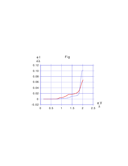
FIG. 1.: The I-V curves for an $SAS$ junction at subgap voltages. The parameters are $\epsilon_{0}=-1.5$, $\Gamma=0.6$, $U=2.4$ (solid curve) and 2.7 (dashed curve).

Subgap current in SAS junctions. In order to find the correlator $\langle\bar{c}c\rangle=i\hat{M}^{-1}$ and the current (27) we numerically inverted the matrix (32) and simultaneously solved the self-consistency equation for $\gamma_{-}$ (30). The resulting $I-V$ characteristics for an $SAS$ junction in the presence of Coulomb interaction are displayed in Fig.1. One observes all the main features predicted within our simple picture of an interplay between MAR and Coulomb interaction: (i) at relatively low voltages $V\leq V_{th}$ MAR current is essentially suppressed due to interaction, (ii) for higher voltages (but still $eV<2\Delta$) MAR is possible and results in a nonzero subgap current which increases with $V$ and (iii) the subharmonic peaks in the differential conductance occur and are shifted to higher voltages as compared to the noninteracting case. An increase of $U$ results in a stronger current suppression and a more pronounced shift of the subharmonic peaks. Close to the gap edge $eV=2\Delta$ the current shoots up sharply.

The parameters used in our numerical analysis are chosen in a way to observe all the key features (i), (ii) and (iii). It is interesting to quantitatively compare the results presented in Fig. 1 with the predictions (1)-(3) of an oversimplified “$E_{C}$-based” model. Let us estimate the effective value of $E_{C}$ (which is, strictly speaking, a function of $U$, $\epsilon_{0}$ $\Gamma$ and $V$ in our calculation) with the aid of eq. (2) and the $I-V$ curves of Fig. 1. We find $E_{C}\approx 0.2\Delta$ for $U=2.4\Delta$ and $E_{C}\approx 0.25\Delta$ for $U=2.7\Delta$. Obviously, these values of $E_{C}$ are smaller than $2\Delta/3$ and, hence, a finite subgap conductance is expected at $eV\gtrsim\sqrt{2\Delta E_{C}}\gg E_{C}$. This is precisely what we observe in Fig. 1. For such values of $V$ and $E_{C}$ eq. (1) yields $n\leq 3$, i.e. only two subharmonic peaks (with $n=2,3$) can occur. This is exactly the case in Fig. 1. Finally, substituting the above values of $E_{C}$ into eq. (3) we can estimate the magnitudes of the peak shifts $\delta V_{n}$. For $U=2.4\Delta$ we find $\delta V_{n}\sim 0.3\Delta$ for $n=2$ and $\sim 0.26\Delta$ for $n=3$. Analogous values for $U=2.7\Delta$ are respectively $\sim 0.38\Delta$ and $\sim 0.33\Delta$. These values are in a reasonably good agreement with our numerical results.

In summary, we presented a detailed analysis of an SAS junction at finite bias and derived its effective action using Keldysh path-integral techniques. Our approach applies for both equilibrium and nonequilibrium current transport in the presence of interactions. The repulsive Coulomb interaction leads to novel effects in the pattern of the subgap current. In particular, it shifts the peaks of the differential conductance toward larger bias. When the interaction is sufficiently strong the subgap current is highly suppressed. Our theoretical predictions can be directly tested in experiments with superconducting quantum dots.

We acknowledge useful discussions with J.C. Cuevas and J. von Delft. This research is supported by DIP German Israel Cooperation project, by the Israeli Science Foundation grant Center of Excellence and by the US-Israel BSF.

REFERENCES

• [1] E. Scheer et al. Phys. Rev. Lett. 78, 3535 (1997).
• [2] J.M. van Ruitenbeek, cond-mat/9910394.
• [3] T.M. Klapwijk, G.E. Blonder, and M. Tinkham, Physica 109+110B, 1157 (1982).
• [4] G. B. Arnold, J. Low Temp. Phys. 59, 143 (1985).
• [5] U. Gunsenheimer and A. D. Zaikin, Phys. Rev. B 50, 6317 (1994).
• [6] D.V. Averin and D. Bardas, Phys. Rev. Lett. 75, 1831 (1995); J.C. Cuevas, A. Marin-Rodero, and A. Levy Yeyati, Phys. Rev. B 54, 7366 (1996); E.N. Bratus, V.S. Shumeiko, and G. Wendin, Phys. Rev. Lett. 74, 2110 (1995).
• [7] L.I. Glazman and K.A. Matveev, Zh. Eskp. Teor. Fiz. Pisma Red. 49, 570 (1989) [JETP Lett. 49, 659 (1989)].
• [8] D.C. Ralph, C.T. Black, and M. Tinkham, Phys. Rev. Lett. 74, 3241 (1995).
• [9] R.P. Feynman and F.L. Vernon Jr., Ann. Phys. (NY) 24, 118 (1963).
• [10] A.O. Caldeira and A.J. Leggett, Phys. Rev. Lett. 46, 211 (1981); Ann. Phys. (NY), 149, 374 (1983).
• [11] G. SchΓΆn and A.D. Zaikin, Phys. Rep. 198, 237 (1990).
• [12] A.V. Rozhkov and D.P. Arovas, Phys. Rev. Lett. 82, 2788 (1999).
• [13] Y. Avishai and A. Golub, Phys. Rev. B 61 11293 (2000).
• [14] L.V. Keldysh, Zh. Eksp. Teor. Fiz. 47, 1515 (1964) [Sov. Phys. JETP 20, 1018 (1965)].