Distribution of consecutive waves in the sandpile model on the Sierpinski gasket

Abstract

The scaling properties of waves of topplings of the sandpile model on a Sierpinski gasket are investigated. The exponent describing the asymptotics of the distribution of last waves in an avalanche is found. Predictions for scaling exponents in the forward and backward conditional probabilities for two consecutive waves are given. All predictions were examined by numerical simulations and were found to be in a reasonable agreement with obtained data.

1 Introduction

Sandpile models form the paradigmatic examples of the concept of self organised criticality (SOC) [1, 2]. This is the phenomenon in which a slowly driven systems with many degrees of freedom evolves spontaneously into a critical state, characterised by long range correlations in space and time.

In the past decade much progress has been made in the theoretical understanding of sandpile models. This is especially true for the Bak-Tang-Wiesenfeld (BTW) model [1, 2], where, following the original work of Dhar [3], a mathematical formalism was developped [4–8] that allows an exact calculation of several properties of the model such as height probabilities [4, 5], the upper critical dimension [8] and so on.

Despite all this work, it has however not been possible yet to give a full and exact characterisation of the scaling properties of the avalanches in the BTW-model. In recent years it has become increasingly clear that, especially in two dimensions, avalanches are to be described by a full multifractal set of scaling exponents [9, 10]. This spectrum of exponents has been calculated with high numerical precision, but at this moment there is no clue how it can be determined by an analytical approach.

Avalanches can be decomposed into simpler objects called waves [7]. The probability distribution of waves seems to obey simple scaling [11] and the exponent describing that scaling is known exactly, both for the general wave [7, 11] and for the last wave of each avalanche[6]. Since in dimensions $d\geq d_{c}=4$, multiple topplings are extremely rare, it is to be expected that in these situations, wave and avalanche statistics obey the same scaling properties.

More recently, the distribution of two consecutive waves has received considerable attention [12, 13]. The conditional probability that the $k+1$-th wave has size $s_{k+1}$ given that the previous wave had size $s_{k}$, $P(s_{k+1}|s_{k})$, is the first quantity to study when one is interested in correlation effects in waves. It are these correlations that make waves and avalanches different. Paczuski and Boettcher [12] proposed, on the basis of extensive simulations, that $P(s_{k+1}|s_{k})$ has a scaling form

$$P(s_{k+1}|s_{k})\sim s_{k+1}^{-\beta}F(\frac{s_{k+1}}{s_{k}})$$ (1)

where for large $x$, $F(x)\sim x^{-r}$, while $F(x)\to\mbox{constant}$ for $x\to 0$. Numerical estimates for these exponents in $d=2$ are $\beta\approx 3/4$, $r\approx 1/2$. At this moment, no exact values for these exponents are known. In a very recent work, Hu et al. [14] study the ‘backward’ conditional probability $P(s_{k}|s_{k+1})$ and find that it obeys a similar scaling law

$$P(s_{k}|s_{k+1})\sim s_{k}^{-\bar{\beta}}\bar{F}(\frac{s_{k}}{s_{k+1}})$$ (2)

where for large $x$, $\bar{F}(x)\sim x^{-\bar{r}}$, while $\bar{F}(x)\to\mbox{constant}$ for $x\to 0$. These authors give arguments that show that

$$\bar{\beta}+\bar{r}=\tau_{lw}$$ (3)

where $\tau_{lw}$ is the scaling exponent describing the size distribution of the last wave. The relation (3) is consistent with the numerical data for the square lattice where both Euclidean and fractal dimensions of waves are $2$. At the same time, it is desirable to get an independent verification of (3) using lattices of different dimensions.

In the present paper we study the properties of waves on the Sierpinski gasket, continuing previous work [15]. Using the methods of analysis introduced in [9], we obtain precise numerical estimates for the exponents $\tau_{lw},\beta,r,\bar{\beta}$ and $\bar{r}$. Also in this case equation (3) seems to be well satisfied which indicates that short time correlations in waves admit an analytical treatment.

2 The sandpile model on a Sierpinski gasket

The BTW sandpile model can be defined on any graph, but for definiteness we will introduce it in the context of the Sierpinski gasket (see figure 1). Each vertex (apart from the three boundary sites) of this graph has four nearest neighbours. To each such vertex $i$ we associate a height variable $z_{i}$ which can take on any positive integer number. We also introduce a critical height $z_{c}$, which we will take equal to four for all vertices. The number of sites in the lattice, $N$, is trivially related to the number of iterations $n$ used in constructing the fractal. The dynamics is defined as follows. On a very slow time scale we drop sand at a randomly selected site and thereby increase the height variable by one: $z_{i}\to z_{i}+1$. When at a given site, $z_{i}>z_{c}$, that site becomes unstable and topples

$$z_{j}\to z_{j}-\Delta_{i,j}$$

where

$$\Delta_{i,j}=\begin{array}[]{rl}4&i=j\\ -1&\mbox{if $i$ and $j$ are nearest neighbours}\\ 0&\mbox{otherwise}\end{array}$$ (7)

Through toppling, neighbouring sites can become unstable, topple themselves, create new unstable sites, and so on. This avalanche of topplings proceeds on a very fast time scale and no new grains of sand are added before the avalanche is over. Sand can leave the system when a boundary site topples. An avalanche is over when all sites are stable again.

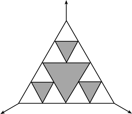
Figure 1: Sierpinski gasket with $n=2$. The arrows indicate the three sites where sand can leave the system.

For further reference it is also necessary to introduce the matrix $G$, called the lattice Green function, which is the inverse of $\Delta$.

It is not difficult to see that the order in which unstable sites are toppled does not influence the stable configuration which is obtained when the avalanche is over. This Abelian nature of the sandpile model allows the introduction of the concept of waves [7] which are introduced in the following way. Suppose that an avalanche starts at a site $i_{0}$ and that after a few topplings $i_{0}$ becomes unstable again. One can then forbid $i_{0}$ to topple again and continue with the toppling of other unstable sites untill all of them are stable. It is easy to show that in such a sequence all sites topple at most once. This set of topplings is called the first wave. Next, we topple the site $i_{0}$ for the second time. If after some topplings it becomes unstable again, we keep it fixed, and topple all the other unstable sites. This set of topplings constitutes the second wave. We continue in this way untill we finally reach a stable configuration. We can in this way decompose any avalanche in a set of waves. The probability distribution $P_{w}(s)$ that an arbitrary wave involves $s$ topplings obeys simple scaling [11]

$$P_{w}(s)\approx s^{-\tau_{w}}$$ (8)

(For the moment we neglect finite size effects which will be taken into account in section 4.)

Because in a wave, sites topple at most once, waves are simpler objects to analyse than avalanches. Without going into details we summarize the following important properties of waves [7]

• There is a one-to-one correspondance between waves and the two-rooted spanning trees on a graph which consists of the Sierpinski gasket and one extra site called the sink. The sink is connected with two edges to each of the three boundary sites of the Sierpinski gasket.

• The element $G_{ij}$ of the Green function is given by the ratio of the number of two-rooted spanning trees (in which $i$ and $j$ are in the same subtree) to the number of one-rooted spanning trees. Moreover $G_{ij}$ is also equal to the expected number of topplings at site $j$ when a grain of sand was dropped at site $i$, which is proportional to the probability that a wave started at $i$ reaches $j$.

From these results, it follows that $P_{w}(R)=dG(R)/dR$ where $R$ is the linear size of the wave. The asymptotic behaviour of the Green function on an arbitrary lattice is

$$G(R)\sim R^{d_{w}-d_{f}}$$

where $d_{f}$ is the fractal dimension of the lattice, and $d_{w}$ the dimension of a random walk on the lattice. Therefore, $P_{w}(R)\sim R^{d_{w}-d_{f}-1}$. From the definition of fractal dimension, $s\sim R^{d_{f}}$ we finally obtain

$$P_{w}(s)\sim s^{d_{w}/d_{f}-2}$$ (9)

so that

$$\tau_{w}=2-\frac{d_{w}}{d_{f}}$$ (10)

a result first derived in [15]. For the particular case of the Sierpinski gasket, $d_{f}=\log{3}/\log{2},d_{w}=\log{5}/\log{2}$, so that $\tau_{w}=\log{(9/5)}/\log{3}\approx 0.535$, a result which is nicely consisted with the available numerical data.

The properties of the last wave in a given avalanche are of special interest for us (see section 3). The probability distribution $P_{lw}(s_{lw})$ that the last wave has $s_{lw}$ topplings obeys the scaling law [11]

$$P_{lw}(s_{lw})\sim s_{lw}^{-\tau_{lw}}$$ (11)

From the definition of waves it follows that the last wave has the property that the site $i_{0}$ is on the boundary of the wave. Let us denote by $d_{B}$ the fractal dimension of the boundary of an arbitrary wave. The number of points on the boundary of a wave of size $s$ is then of order $s^{d_{B}/d_{f}}$. Hence, the probability that a given site is on the boundary of a wave of size $s$ is proportional to $s^{d_{B}/d_{f}-1}$, which should also be proportional to $P_{lw}(s_{lw})/P_{w}(s)$. Using (6) we immediately obtain

$$\tau_{lw}=3-\frac{d_{w}+d_{B}}{d_{f}}$$ (12)

In two dimensions, $d_{w}=2$ and $d_{B}=z=5/4$ where $z$ is the fractal dimension of the chemical path on a spanning tree. One thus finds $\tau_{lw}=11/8$ [6]. On a fractal the relation between $d_{B}$ and $z$ may be more complicated. In fact, it was shown in [16] that for a deterministic fractal

$$d_{B}=z-d_{w}+d_{f}$$ (13)

so that, from (12) we obtain

$$\tau_{lw}=2-\frac{z}{d_{f}}$$ (14)

The exponent $z$ on the Sierpinski gasket was also calculated in [16] with the result
$z=\log{[(20+\sqrt{205})/15]}/\log{2}$. Thus one finally obtains for the case of the Sierpinski gasket

$$\tau_{lw}=-\frac{\log{[(20+\sqrt{205})/135]}}{\log{3}}\approx 1.247$$ (15)

In section 4, we will present numerical estimates for $\tau_{lw}$ that are fully consistent with this prediction .

3 Distribution of consecutive waves

In order to characterise the statistical properties of waves more completely, it is necessary to go beyond the description on the basis of the distribution $P_{w}(s)$ only. Following the work of Paczuski and Boettcher [12] we now turn to a study of the conditional probability $P(s_{k+1}|s_{k})$ where $s_{k}$ is the size of the $k$-th wave. If the size of consecutive waves is a Markov process, this conditional probability is sufficient to describe the evolution of wave sizes. In figure 2.a, we show our data for this conditional probability for Sierpinski gaskets with $n=9$ ($N=29526$). All our data were obtained by studying at least $1000\times N$ avalanches. The figure shows the best fit of our data to the scaling form (1) proposed by Paczuski and Boettcher. Unfortunately, it is not possible to obtain very accurate estimates for the exponents $\beta$ and $r$ in this way. We will come back to this issue in the next section.

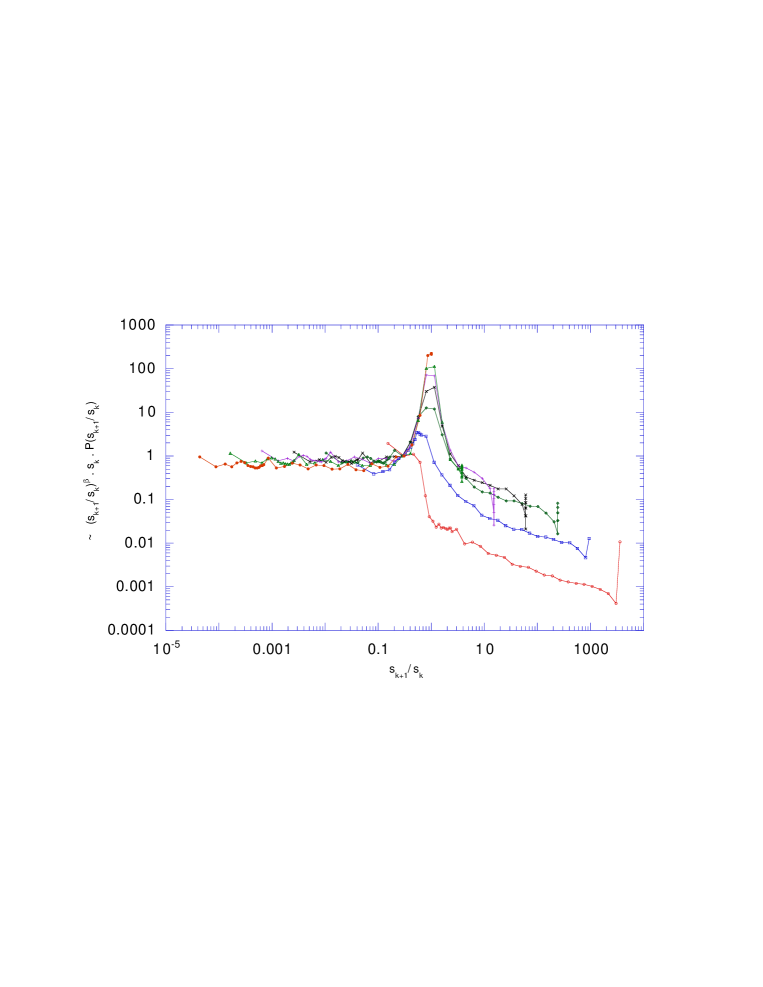
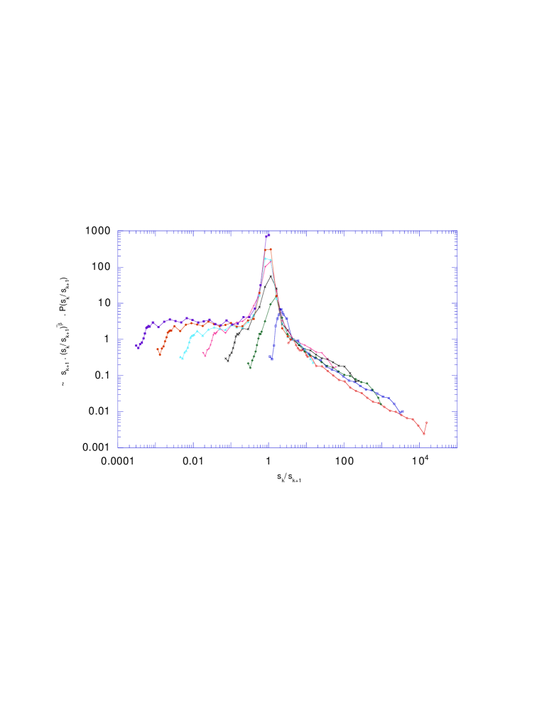
Figure 2: Scaled conditional probabilities $P(s_{k+1}|s_{k})$ (a) and $P(s_{k}|s_{k+1})$ (b). The results were obtained for a Sierpinski gasket with $n=9$.

Recently, it was pointed out that the ‘backward’ conditional probability $P(s_{k}|s_{k+1})$ is also of interest because it is possible to relate the exponents $\bar{\beta}$ and $\bar{r}$ (see (2)) to $\tau_{lw}$. In figure 2.b we present our data for this quantity, again for the case $n=9$.

We now repeat briefly the argument given in [14]. We begin by rewriting (2) in a normalised form

$$P(s_{k}|s_{k+1})\sim\left(\frac{s_{k}}{s_{k+1}}\right)^{-\bar{\beta}}\bar{F}\left(\frac{s_{k}}{s_{k+1}}\right)\ s_{k+1}^{-1}$$ (16)

Let’s next consider the situation in which $s_{k}\gg s_{k+1}$ so that the argument of $\bar{F}$ in (16) is large. In that case it must be so that the $(k+1)$-th wave has a non-empty intersection with the boundary of the previous wave (see figure 3.a). Indeed, assume the opposite so that the $(k+1)$-th wave covers a small region inside the much bigger $k$-th wave (figure 3.b). But such a situation is forbidden, since all sites inside the $k$-th wave return to their original height after the wave has passed. The $(k+1)$-th wave must therefore follow the motion of the previous wave untill it hits the boundary of the $k$-th wave from where it can follow a different evolution. Therefore, the situation of figure 3.b cannot occur.

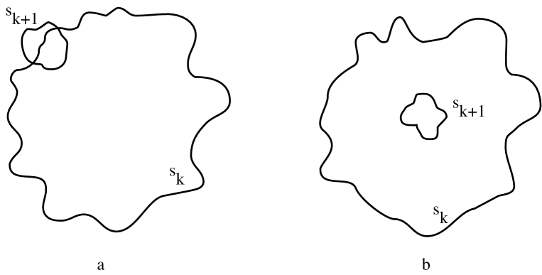
Figure 3: When $s_{k+1}\ll s_{k}$ the $k+1$ the wave must have an intersection with the boundary of the $k$-th wave as shown in a. The situation in b cannot occur.

Then, consider figure 3.a on a coarse grained scale by performing a rescaling of the order of $R_{k+1}$, the linear size of the $k+1$-th wave. On that scale, the geometry of figure 3.a resembles that of last waves with $s_{k+1}$ playing the role of the origin of the avalanche, and $s_{k}$ that of the last wave. Hence we arrive at the conclusion that in the limit $s_{k}\gg s_{k+1}$, the distribution of $s_{k}$ coincides with that of the last wave. From (16), (11) and the asymptotic behaviour of $\bar{F}$, the equality (3) then follows.

Once this result has been obtained it is possible to obtain also a relation for the exponents $\beta$ and $r$ that appear in the scaling form (1). The joint distribution $P(s_{k},s_{k+1})$ can be written in two ways using either the forward or backward conditional probability

$$P(s_{k},s_{k+1}) = P(s_{k}|s_{k+1})P_{w}(s_{k+1})$$

$$= P(s_{k+1}|s_{k})P_{w}(s_{k})$$

We then insert (16), (8) and a properly normalised version of (1) and get

$$\left(\frac{s_{k}}{s_{k+1}}\right)^{-\bar{\beta}}\bar{F}\left(\frac{s_{k}}{s_{k+1}}\right)\ s_{k+1}^{-1-\tau_{w}}\sim\left(\frac{s_{k+1}}{s_{k}}\right)^{-\beta}F\left(\frac{s_{k+1}}{s_{k}}\right)\ s_{k}^{-1-\tau_{w}}$$ (17)

In the case $s_{k}\gg s_{k+1}$ we insert the proper limiting behaviours of the functions $F$ and $\bar{F}$, and immediately obtain, using (3)

$$\beta=1+\tau_{w}-\tau_{lw}$$ (18)

A final equality between exponents can be obtained by investigating the limit $s_{k}\ll s_{k+1}$ in (17). Inserting the appropriate scaling behaviours one obtains

$$\beta+r=1+\tau_{w}-\bar{\beta}$$ (19)

In $d=2$, (18) leads to the predictions $\beta=5/8$ and $\bar{\beta}+\bar{r}=11/8$. The value of $\beta$ is not too far from the numerical estimate $\beta\approx 3/4$ reported by [12], while in [14] numerical evidence is presented that is in agreement with the prediction (3). In the following section, we investigate the situation on the Sierpinski gasket.

4 Numerical results

In order to analyse our data we have used the method introduced in [9], in which one investigates the moments $\langle s^{q}\rangle$ of the distribution $P(s,L)$, where we now explicitly take into account the size $L$ of the system. In our case, $L=2^{n}$. If $P(s,L)$ has a simple scaling form

$$P(s,L)\sim s^{-\tau}H(s/L^{d_{f}})$$ (20)

these moments should be proportional to simple powers of $L$, $\langle s^{q}\rangle\sim L^{\sigma(q)}$ where $\sigma(q)=d_{f}(1-\tau+q)$ for $q>\tau-1$, and $\sigma(q)=0$ for $q\leq\tau-1$.

In principle, an analysis of the moments is most instructive when one is interested in the presence of possible multifractal scaling (instead of simple scaling). In that case, the function $\sigma(q)$ becomes nonlinear. However, even in the absence of multifractality, this kind of analysis has many advantages. In the case of Sierpinski gasket, the probability distributions for the size of avalanches, waves and last waves show strong oscillations superposed on the pure power laws (see the figures 2,4 and 5 in [15]) . This is a consequence of the discrete scale invariance of the system. These oscillations make the determination of the scaling exponents a hard task. The moments $\langle s^{q}\rangle$ have the big advantage that they are averages over the distribution and hence the effects of the oscillations almost completely disappear. If one then assumes simple scaling, as we know is correct for waves [11], one can further reduce any remaining fluctuations by fitting the values of $\sigma(q)$ (for $q$ big enough) to a straight line. The slope of the line should equal $d_{f}$, and the intersection with the $q$-axis gives $\tau-1$.

We tested this method of analysis for the last wave. We performed extensive simulations for Sierpinski gaskets with $5\leq n\leq 9$. From the statistics of the last waves we could then estimate $\sigma_{lw}(q)$. The results are shown in figure 4. The curvature at low $q$ is a finite size effect. From a fit of our data in the regime $q\geq 1.5$ we obtain the estimate $\tau_{lw}=1.28\pm.03$. This is very close to the exact result which we obtained in section 2 .

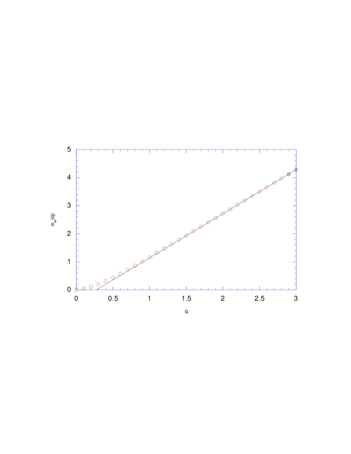
Figure 4: The moment exponent $\sigma_{lw}(q)$ for last waves. The straight line gives a best fit to the high $q$-data, from which $\tau_{lw}$ can be obtained.

We have followed a similar scheme of analysis for all the other exponents introduced in section 3. Take as a concrete example the sum of exponents $\bar{\beta}+\bar{r}$. This can be obtained as follows. For $s_{k}\gg s_{k+1}$, $P^{+}(s_{k})\equiv P(s_{k}|s_{k+1})\sim s_{k}^{-\bar{r}-\bar{\beta}}$. Instead of analysing this distribution itself we look at the moments of $P^{+}(s_{k})$ which are expected to scale as $L^{\sigma^{+}(q)}$. A plot of $\sigma^{+}(q)$ is shown in figure 5. From an analysis of the data in this figure we obtain the estimate $\bar{\beta}+\bar{r}=1.24\pm.01$, which is very clearly consistent with the prediction (3).

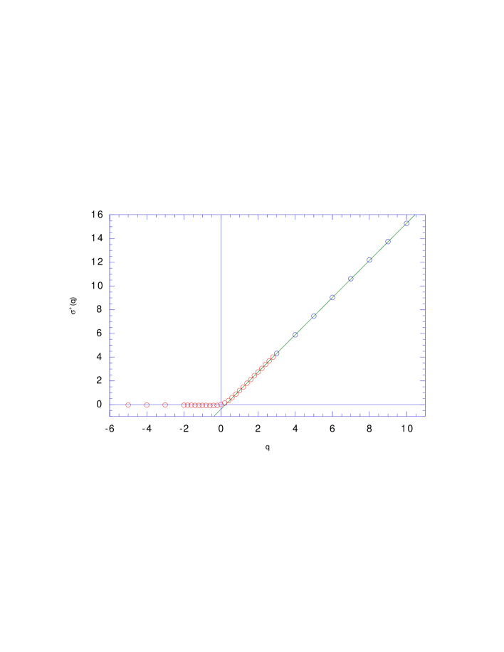
Figure 5: The moment exponent $\sigma^{+}(q)$ (see text). The straight line gives a best fit to the high $q$-data, from which $\bar{\beta}+\bar{r}$ can be obtained.

By analysing the small $s_{k}$ behaviour of $P(s_{k}|s_{k+1})$ in a similar way, we can estimate $\bar{\beta}=.16\pm 0.05$.

Continuing in this way for the forward conditional probability $P(s_{k+1}|s_{k})$, we find from the large $s_{k+1}$-behaviour $\beta+r=1.30\pm 0.01$, while from the data for small $s_{k+1}$ we finally obtain $\beta=0.35\pm 0.05$ (see figure 6). This numerical result is not too different from the prediction following from (18) which gives $\beta=.288$.

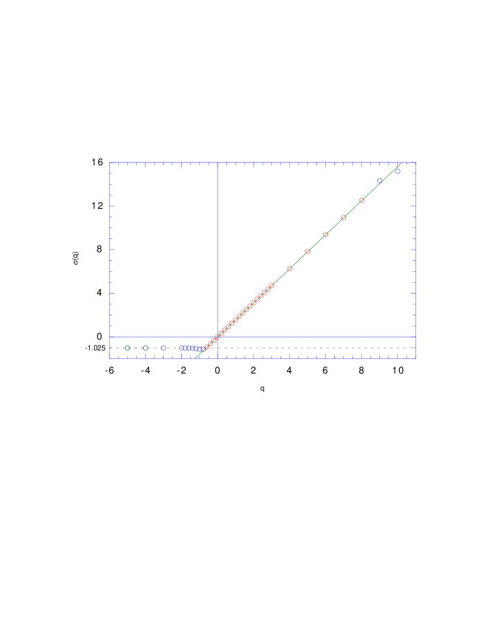
Figure 6: The exponents of the moments of $P(s_{k+1}|s_{k})$ for $s_{k+1}\ll s_{k}$. The straight line gives a best fit to the high $q$-data from whicht the exponent $\beta$ can be estimated

Finally note that also the relation (19) is rather well satisfied.

5 Conclusions

In this paper we investigated the properties of waves in the sandpile model on a Sierpinski gasket. We gave predictions for the exponent describing the last wave in an avalanche and for the scaling exponents occuring in forward and backward conditional probabilities for consecutive waves. These predictions were tested by extensive simulations and were found to be in good agreement with the numerics.

Results such as those shown in figure 5 and figure 6 also show no clear evidence for any multifractality which would show up as a curvature in the plots of $\sigma(q)$ for big enough $q$ ([10]).

We are currently investigating the presence of multifractality of avalanches on the Sierpinski gasket. If, as is the case in $d=1$ ([17]) and in $d=2$ ([9, 10]), such multifractality shows up , the interesting question arises how such a phenomenon can be built up on the avalanche level when it is absent at the level of waves and consecutive waves.

Acknowledgement One of us (VBP) thanks the Limburgs Universitair Centrum for hospitality.

References

- [1] Bak P., Tang C., Wiesenfeld K., Phys. Rev. Lett. 59, 381 (1987).
- [2] Bak P., Tang C., Wiesenfeld K., Phys. Rev. A 38, 364 (1988).
- [3] Dhar D., Phys. Rev. Lett. 64, 1613 (1990).
- [4] Majumdar S.N., Dhar D., Physica A 185, 129 (1992).
- [5] Priezzhev V. B., J. Stat. Phys. 74, 955 (1994).
- [6] Dhar D., Manna S.S. Phys. Rev. E 49, 2684 (1994).
- [7] Ivashkevich E.V., Ktitarev D.V., Priezzhev V.B., Physica A 209, 347 (1994).
- [8] Priezzhev V.B., preprint cond-mat/9904054
- [9] De Menech M., Stella A.L., Tebaldi C., Phys. Rev. E 58, 2677 (1998).
- [10] Tebaldi C., De Menech M., Stella A.L., Phys. Rev. Lett. 83, 3952, (1999).
- [11] Ktitarev D.V., Lübeck S., Grassberger P., Priezzhev V.B., preprint cond-mat/9907157.
- [12] Paczuski M., Boettcher S., Phys. Rev. E 56, R3745 (1997).
- [13] Ktitarev D.V., Priezzhev V.B., Phys. Rev. E 58, 2883 (1998).
- [14] Hu C.-K., Ivashkevich E.V., Lin C.-Y., Priezzhev V.B., preprint cond-mat/9908089.
- [15] Daerden F., Vanderzande C., Physica A 256, 533 (1998).
- [16] Dhar D., Dhar A., Phys. Rev. E 55, R2093 (1997).
- [17] Kadanoff L.P., Nagel S.R., Wu L., Zhou S., Phys. Rev. A 39, 6524 (1989).