Binary hard-sphere fluids near a hard wall

Abstract

By using the Rosenfeld density functional we determine the number density profiles of both components of binary hard-sphere fluids close to a planar hard wall as well as the corresponding excess coverage and surface tension. The comparison with published simulation data demonstrates that the Rosenfeld functional, both its original version and sophistications thereof, is superior to previous approaches and exhibits the same excellent accuracy as known from studies of the corresponding one-component system.

I Introduction

A variety of experimental techniques has emerged which allow one to resolve the inhomogeneous density distributions of fluids at interfaces, a subject which enjoys broad scientific interest. In this context the ability to manufacture highly monodisperse colloidal suspensions has turned out to be particular useful as they provide the possibility to tune the effective interactions in these systems such that, e.g., the colloidal particles closely resemble hard-sphere fluids [1] . Since many of these experimental probes are indirect scattering techniques there is a substantial demand to guide them theoretically. Computer simulations and integral theories [2] are important tools of statistical physics to address these issues. Density functional theory (DFT) [3] has emerged as an additional approach which is capable to capture interfacial phase transitions and to sweep the thermodynamic and interaction parameter space of the system under consideration. The potential to combine these two possibilities poses already a major challenge for the other techniques. If DFT acquires in addition the same accuracy as the other two techniques, it could gain a clear competitive edge.

Although there is no recipe for constructing systematically a reliable DFT in spatial dimensions $d\geq 2$, the constant flux of developments over many years has led to a rather high level of sophistication. Among these theories for hard-sphere fluids, which act as paradigmatic systems and stepping-stones for more complicated models, the Rosenfeld functional has emerged as a particular powerful theory which resorts to the fundamental geometrical measures of the individual sphere [4]. For the standard test case of the highly inhomogeneous density distribution of a one-component hard-sphere fluid near a planar hard wall, the predictions of the Rosenfeld functional are very close to those of numerical simulations serving as benchmarks. For this case the mean square deviations [see, c.f., Eq. (22)] of Rosenfeld DFT results from the simulation data from Ref. [5] are at most $1\times 10^{-3}$ at high packing fractions, otherwise less than $3\times 10^{-4}$.

Another virtue of the Rosenfeld functional is that is easily lends itself to the generalization to multi-component hard-sphere fluids. This opens the door to investigate rich new physical phenomena as particles of different size compete for interfacial positions [6]. Even for the simplest multi-component system, the binary hard-sphere fluid, there are only relatively few theoretical studies which determine their structural properties near a planar hard wall, using Monte Carlo simulations [7, 8, 9, 10], integral equation theories [9], and various kinds of density functional theory [8, 9, 10, 11, 12, 13, 14, 15], as well as in spherical pores [16]. Here we analyze this problem by using the corresponding Rosenfeld functional both in its original version [4] as well as for sophistications thereof [17, 18]. By comparing these results with published simulation data [10] we assess to which extent the quantitative reliability of the Rosenfeld functional for the one-component hard-sphere fluid remains valid for the corresponding binary system. Moreover we determine concentration profiles, the excess coverage, and the surface tension of the binary hard-sphere fluids at a hard wall. We describe the DFT in Sec. II and report our results in Sec. III followed by a summary and our conclusions in Sec. IV. The Appendix contains important technical details.

II Density functional theory

The Rosenfeld functional for the excess (over the ideal gas) Helmholtz free energy of a mixture of hard spheres with number density profiles $\{\rho_{i}({\bf r})\},~i=1,\dots,N$, can be written as [4]

$$\beta{\cal F}_{ex}[\{n_{\alpha}\}]=\int{\mathrm{d}}^{3}r~\Phi(\{n_{\alpha}({\bf r})\})$$ (1)

which is a functional of the four scalar weighted densities $n_{\alpha}({\bf r})$ for the $N$-component mixture

$$n_{\alpha}({\bf r})=\sum_{i=1}^{N}\int{\mathrm{d}}^{3}r^{\prime}~\rho_{i}({\bf r^{\prime}})~\omega_{i}^{(\alpha)}({\bf r}-{\bf r}^{\prime}),~\alpha=0,\dots,3,$$ (2)

with $4N$ scalar weight functions $\omega_{i}^{(\alpha)}$ and two three-component vector weighted densities ${\bf n}_{\alpha}({\bf r})$

$${\bf n}_{\alpha}({\bf r})=\sum_{i=1}^{N}\int{\mathrm{d}}^{3}r^{\prime}~\rho_{i}({\bf r^{\prime}})~\mbox{\boldmath$\omega$}_{i}^{(\alpha)}({\bf r}-{\bf r}^{\prime}),~\alpha=1,2,$$ (3)

with $2N$ vector weight functions $\omega$${}_{i}^{(\alpha)}$. The weight functions contain only information about the fundamental geometrical measures of a single sphere of species $i$, namely its volume, surface area, and radius $R_{i}$, i.e., in particular they are independent of the density profiles. The explicit expressions for the weight functions are given in the Appendix. $\Phi(\{n_{\alpha}\})=\Phi_{1}+\Phi_{2}+\Phi_{3}$ is a function of the weighted densities with [4]

$$\Phi_{1} = -n_{0}\log(1-n_{3}),$$ (4)

$$\Phi_{2} = \frac{n_{1}n_{2}-{\bf n}_{1}\cdot{\bf n}_{2}}{1-n_{3}},$$ (5)

and

$$\Phi_{3} = \frac{\frac{1}{3}n_{2}^{3}-n_{2}{\bf n}_{2}\cdot{\bf n}_{2}}{8\pi(1-n_{3})^{2}}=\frac{n_{2}^{3}}{24\pi(1-n_{3})^{2}}~(1-3\xi^{2}),$$ (6)

where $\xi({\bf r})\equiv|{\bf n}_{2}({\bf r})|/n_{2}({\bf r})$, which is the ratio of the modulus of the vector weighted density ${\bf n}_{2}({\bf r})$ and the scalar weighted density $n_{2}({\bf r})$. We want to note that $\xi({\bf r})\equiv 0$ in the bulk and is small for small inhomogeneities. While this original Rosenfeld functional describes very successfully the fluid phase of a one-component hard-sphere system [19], it fails to predict the freezing transition. This failure has been studied in detail in Refs. [17] and [18]. For the freezing transition it turns out that the zero-dimensional limit of the functional, in which a small cavity can accommodate only a single sphere, plays a key role. In a crystal the thermal vibrations around a lattice site can be interpreted as the motions in such a cavity formed by the neighboring spheres. Only if the statistical mechanics in such a cavity is described properly by the density functional, the freezing transition is predicted correctly. This is not the case for the original Rosenfeld functional. This problem can be fixed by modifying slightly the contribution $\Phi_{3}$ [see Eq. (6)] such that the freezing transition is predicted by the modified functional while at the same time, for lower packing fractions, the accuracy of the original functional in describing the inhomogeneous fluid is kept. The following modifications have been suggested [17, 18]:

$$\Phi_{3,q}=\frac{n_{2}^{3}}{24\pi}~(1-\xi^{2})^{q}$$ (7)

with $q\geq 2$ and

$$\Phi_{3,int}=\frac{n_{2}^{3}}{24\pi}~(1-3\xi^{2}+2\xi^{3}).$$ (8)

The first suggestion, $\Phi_{3,q}$, is an antisymmetrized version of $\Phi_{3}$ in Eq. (6) and the second, $\Phi_{3,int}$, interpolates between $\Phi_{3}$ of Eq. (6) and $\Phi_{3,0D}$ in the exact zero-dimensional limit

$$\Phi_{3,0D}=\frac{n_{2}^{3}}{24\pi(1-n_{3})^{2}}~\xi(1-\xi)^{2}.$$ (9)

While the modified Rosenfeld function with $\Phi_{3,0D}$ does successfully predict the freezing transition of the one-component system, it leads to modified bulk properties and hence cannot describe the hard-sphere fluid as accurate as the original Rosenfeld functional. We note that the difference between $\Phi_{3}$ of the original Rosenfeld functional and both $\Phi_{3,q}$ with $q=3$ and $\Phi_{3,int}$ is of the order of ${\cal O}(\xi^{3})$. Therefore we expect the biggest differences between the various versions of the Rosenfeld DFT to occur close to the wall where $\xi$ is largest.

Both the original Rosenfeld functional and the modifications corresponding to Eqs. (7) and (8), i.e., the functionals that share common bulk properties, are very successful and accurate for the one-component fluid. But far less is known for binary mixtures. While in this latter respect in Ref. [20] very good agreement between the density profiles obtained from the Rosenfeld functional and simulation data from Ref. [7] has been mentioned, in a recent study [10] significant deviations between the Rosenfeld DFT results and simulations have been found. In this latter study an alternative but equivalent formulation [21, 22] of the original Rosenfeld functional has been applied.

Here we are interested in the equilibrium density profiles $\rho_{s,0}({\bf r})$ and $\rho_{b,0}({\bf r})$ of both the small and big components of binary hard-sphere mixtures close to a planar hard wall. To this end we freely minimize the functional

$$\Omega[\rho_{s}({\bf r}),\rho_{b}({\bf r})]={\cal F}[\rho_{s}({\bf r}),\rho_{b}({\bf r})]+\sum_{i=s,b}\int{\mathrm{d}}^{3}r^{\prime}~\rho_{i}({\bf r}^{\prime})\left(V_{ext}^{i}({\bf r}^{\prime})-\mu_{i}\right)$$ (10)

which is written in terms of the functional

$${\cal F}[\rho_{s}({\bf r}),\rho_{b}({\bf r})]={\cal F}_{id}[\rho_{s}({\bf r}),\rho_{b}({\bf r})]+{\cal F}_{ex}[\rho_{s}({\bf r}),\rho_{b}({\bf r})]$$ (11)

with the exactly known ideal gas contribution ${\cal F}_{id}$,

$$\beta{\cal F}_{id}=\sum_{i=s,b}\int{\mathrm{d}}^{3}r^{\prime}~\rho_{i}({\bf r}^{\prime})\left(\ln(\lambda_{i}^{3}\rho_{i}({\bf r}^{\prime}))-1\right),$$ (12)

with $\lambda_{i}$ the thermal wave length of species $i$. For the equilibrium density profiles $\rho_{i,0}({\bf r})$, $i=s,b$, the functionals ${\cal F}$ and $\Omega$ reduce to the Helmholtz free energy and the grand canonical potential of the mixture, respectively; $\mu_{s}$ and $\mu_{b}$ are the chemical potentials of the two species. The external potentials entering into Eq. (10) model the planar hard wall at $z=0$:

$$V_{ext}^{i}(z)=\left\{\begin{array}[]{rl}\infty,&z<R_{i},\\ 0,&\mbox{otherwise},\end{array}\right.$$ (13)

$i=s,b$, with $z$ the normal distance from the wall. The external potentials prevent the centers of spheres of species $i$ to approach the wall, located at $z=0$, closer than $R_{i}$ in which case they are in contact.

In the absence of spontaneous symmetry breaking due to freezing, which we do not consider here, the profiles $\rho_{i,0}(z)$, $i=s,b$, depend only on the normal coordinate $z$ which simplifies the minimization of the functional.

Far away from the wall, i.e., in the bulk system, the vector weighted densities ${\bf n}_{1}$ and ${\bf n}_{2}$ and thus $\xi$ vanish. In this limit both the original Rosenfeld functional and the two modifications corresponding to Eqs. (7) and (8) reduce to the same bulk expression given by

$$\Phi_{bulk}=-n_{0}\ln(1-n_{3})+\frac{n_{1}n_{2}}{1-n_{3}}+\frac{n_{2}^{3}}{24\pi(1-n_{3})^{2}}$$ (14)

and hence they share the same bulk properties. We want to emphasize that as a consequence of this feature all versions of the Rosenfeld functional predict density profiles which show the same asymptotic decay towards the bulk value [23]. The weighted densities in the bulk limit are obtained by inserting the bulk densities $\rho_{i,bulk}:=\rho_{i,0}(z=\infty)$ into Eq. (2) yielding

$$n_{3} = \frac{4\pi}{3}\sum_{i=s,b}R_{i}^{3}\rho_{i,bulk}\equiv\sum_{i=s,b}\eta_{i},$$ (15)

$$n_{2} = 4\pi\sum_{i=s,b}R_{i}^{2}\rho_{i,bulk},$$ (16)

$$n_{1} = \sum_{i=s,b}R_{i}\rho_{i,bulk},$$ (17)

and

$$n_{0} = \sum_{i=s,b}\rho_{i,bulk}.$$ (18)

The equation of state following from Eq. (14),

$$\beta p=\frac{n_{0}}{1-n_{3}}+\frac{n_{1}n_{2}}{(1-n_{3})^{2}}+\frac{1}{12\pi}\frac{n_{2}^{3}}{(1-n_{3})^{3}},$$ (19)

is the Percus-Yevick compressibility equation of state of the mixture [24]. This expression is related to the contact values of the density profiles according to the sum rule [25]

$$\beta p=\sum_{i=s,b}\rho_{i}(z=R_{i}+0).$$ (20)

This sum rule is respected by the Rosenfeld functional as by any weighted-density DFT [26] and therefore provides a test for the numerical accuracy of the calculations. In the following we suppress the subscript 0 which indicates equilibrium profiles as opposed to variational functions.

III Structural and thermodynamic properties

A Density profiles

The number density profiles of both components of binary hard-sphere mixtures close to a planar hard wall are obtained by a free minimization of the functional given in Eq. (10). We use the original Rosenfeld functional as well as the modified versions corresponding to Eq. (8) and to Eq. (7) with $q=2$ and $q=3$. The systems considered here have two different size ratios, $R_{b}:R_{s}=5:3$ and $R_{b}:R_{s}=3:1$, and various packing fractions $\eta_{s}$ and $\eta_{b}$ of the small and big spheres [27], respectively. The resulting density profiles are compared with simulation data published in Ref. [10]. In addition we calculate the local concentrations $\Phi_{s}(z)$ and $\Phi_{b}(z)$ of the small and big spheres, respectively, defined as

$$\Phi_{i}(z)=\frac{\rho_{i}(z)}{\rho_{s}(z)+\rho_{b}(z)},~i=s,b.$$ (21)

We find excellent agreement between the density profiles of both components obtained by density functional theory and the simulation data for all systems under consideration. This holds for all versions of the Rosenfeld functional analyzed here. While at low total packing fractions $\eta=\eta_{s}+\eta_{b}$ the density functional theory results for all versions of the Rosenfeld functional are practically equivalent, small deviations among the results from different versions of the functional appear at larger values of $\eta$, i.e., for $\eta\gtrsim 0.3$. We quantify the degree of agreement between our DFT density profiles $\rho_{i}(z)$ and the simulation data from Ref. [10], available as data points $(z_{j},\rho_{i}^{sim}(z_{j}))$, $j=1\dots N_{i}^{sim}$ and $i=s,b$, by determining the mean square deviations $\bar{E}_{i}$, $i=s,b$, defined as

$$\bar{E}_{i}=\frac{1}{N_{i}^{sim}}\sum_{j=1}^{N_{i}^{sim}}\left(\frac{\rho_{i}^{sim}(z_{j})-\rho_{i}(z_{j})}{\rho_{i,bulk}}\right)^{2}.$$ (22)

We find that $\bar{E}_{s}$ and $\bar{E}_{b}$ are at most $5\times 10^{-4}$ and $6\times 10^{-3}$, respectively, for all versions of the Rosenfeld functional. However, since the statistical errors in the simulation data are comparable with or even larger than the differences between the density profiles obtained by different version of the Rosenfeld DFT this approach does not enable us to determine which of the various versions is the most accurate one.

To illustrate the agreement between the DFT and the simulation data, in Fig. 1 we show the density profiles of the small spheres (a) and of the big spheres (b) for $\eta_{s}=0.0607$ and $\eta_{b}=0.3105$ and a size ratio $R_{b}:R_{s}=5:3$. The symbols ($\square$) denote the simulation data from Ref. [10] and the solid line is obtained by the original Rosenfeld functional. The dotted lines denote coarse grained densities $\bar{\rho}_{i}^{(j)}$, $i=s,b$ and $j=0,1$, defined as

$$\bar{\rho}_{i}^{(j)}=\frac{1}{z_{i}^{(j+1)}-z_{i}^{(j)}}\int\limits_{z_{i}^{(j)}}^{z_{i}^{(j+1)}}{\mathrm{d}}z~\frac{\rho_{i}(z)}{\rho_{i,bulk}},$$ (23)

with $z_{i}^{(0)}\equiv 0$ and $z_{i}^{(j>0)}$ the position of the $j$th minimum [28]. All details of the density profiles found in the simulations are reproduced very accurately by the density functional theory. The oscillatory behavior, i.e., the amplitudes, the phases, and the decay of the oscillations as obtained by DFT agree excellently with the simulations. The total packing fraction of the system $\eta=\eta_{s}+\eta_{b}=0.3712$ is already rather high, giving rise to the pronounced structure of the density profiles. The corresponding concentration profiles $\Phi_{s}(z)$ and $\Phi_{b}(z)$ of the small and big spheres, respectively, are shown in Fig. 2. These concentration profiles demonstrate that, apart from the purely geometrical constraints, near the wall the big particles are enriched and the small particles depleted. This is in line with the expectation based on the attractive depletion potential near a hard wall of a single big sphere immersed in a fluid of small spheres [30]. Correlation effects reverse this relative distribution in the second layer and restore it in the third.

As mentioned above, small differences between the DFT results corresponding to the various versions of the Rosenfeld functional can be found for these values of $\eta$. In order to be able to resolve these small differences magnified parts of the density profiles from Fig. 1 are shown in Fig. 3 together with the simulation data from Ref. [10]($\square$). The solid lines in Fig. 3 correspond to the original Rosenfeld functional, the dotted lines correspond to the interpolated version [Eq. (8)] whereas the dashed and dashed-dotted lines correspond to the antisymmetrized version [Eq. (7)] with $q=2$ and $q=3$, respectively. All DFT results are very close to the simulation data. However, the deviations between the simulations and the antisymmetrized functional with $q=2$ seem to be systematically the largest.

In Figs. 4 and 5 we show the density profiles of a binary mixture with size ratio $R_{b}:R_{s}=3:1$. The packing fraction of the small spheres is $\eta_{s}=0.0047$ and that of the big spheres is $\eta_{b}=0.3859$ so that the total packing fraction $\eta=\eta_{s}+\eta_{b}=0.3906$ is again rather high. Therefore there is a strong spatial variation of the density profiles. The agreement between DFT (solid line) and simulations ($\square$) is again found to be excellent for both the density profile of the small spheres (a) and of the big spheres (b). The dotted lines denote the coarse grained densities as defined in Eq. (23)[29]. The concentrations profiles of the small and big spheres, corresponding to these density profiles are shown in Fig. 6. For this larger size ratio the anti-correlated behavior of $\Phi_{s}(z)$ and $\Phi_{b}(z)$ is even more pronounced than for the smaller ratio discussed in Fig. 2 and strongly locked in without additional fine structure such as the double peak appearing in Fig. 2.

In addition we test the numerical accuracy of our calculations by means of the sum rule given in Eq. (20). In Table I the sum of the contact values of the binary mixture with size ratio $R_{b}:R_{s}=5:3$ for various packing fractions is compared with two equations of state. $\beta p_{PY}^{c}$ denotes the Percus-Yevick compressibility equation of state [Eq. (19)], to which the Rosenfeld functional reduces in the bulk limit, and $\beta p_{MCSL}$ corresponds to the more accurate Mansoori-Carnahan-Starling-Leland equation of state [31], which represents a generalization to a mixture of the very accurate Carnahan-Starling equation of state [32] for the one-component fluid. The very good agreement between the contact values and $\beta p_{PY}^{c}$ demonstrates the high accuracy of our numerical procedure. However, at higher packing fractions, $\beta p_{PY}^{c}$ deviates from the more accurate equation of state $\beta p_{MCSL}$. The same analysis of our results for a binary mixture with size ratio $R_{b}:R_{s}=3:1$ is summarized in Table II.

Equation (20) represents a sum rule which must be fulfilled by the density profiles as obtained by any of the density functionals considered here. However, no corresponding rules are available for the individual contact values. We find that for all versions of the Rosenfeld functional under consideration here, the sum rule is respected equally well. However, the individual contact values may differ. This statement is in line with the expectation that the biggest differences between the various versions of the Rosenfeld functional occur in a region where $\xi$ is large, i.e., close to the wall, and is substantiated in Table III for the binary mixture with size ratio $R_{b}:R_{s}=5:3$ and in Table IV for the size ratio $R_{b}:R_{s}=3:1$.

Vested with this confidence in our numerical procedures we are now able to comment on the comparison of our DFT results for the original Rosenfeld functional with those obtained by earlier DFT studies [8, 9, 10, 11, 12, 13, 14, 15]. We find that DFT approaches other than the Rosenfeld DFT predict the structure of the density profiles of a binary hard-sphere mixture near a planar hard wall only qualitatively [8, 9, 11, 12, 13, 14, 15], whereas the Rosenfeld functional yields quantitatively reliable predictions. This is demonstrated by Figs. 1 and 3–5 and the very small values of the mean square deviations $\bar{E}_{s}$ and $\bar{E}_{b}$ [Eq. (22)]. The predictions of the Rosenfeld functional agree excellently in all details with the simulation results from Ref. [10]. The deviations between the DFT results of Ref. [10], calculated with the Rosenfeld functional, and their own simulations originate most likely from numerically problems of the iteration procedure used in Ref. [10]. This suspicion is further supported by the fact that the DFT density profiles shown in Ref. [10] seem to violate the sum rule Eq. (20). Thus we are led to the conclusion that the deviations between the Rosenfeld DFT results and the simulation data reported in Ref. [10] most likely are artifacts generated by numerical problems in implementing the iteration procedure used in Ref. [10] for solving the Euler-Lagrange equations corresponding to the Rosenfeld density functional. Therefore the doubts raised in Ref. [10] about the performance of the Rosenfeld DFT for binary hard-sphere mixtures are not justified. We conclude that the Rosenfeld DFT exhibits the same high accuracy in predicting density distributions of binary hard-sphere mixtures as for the one-component hard-sphere fluid.

B Excess adsorption and surface tension

One of the virtues of DFT is that based on the knowledge of the local structural properties $\rho_{i}(z)$, $i=s,b$, it is straightforward to calculate also thermodynamic properties such as the excess adsorptions $\Gamma_{i}$ and the surface tension $\gamma$. Here we determine these quantities near a hard wall for a binary hard-sphere fluid whose components exhibits a size ratio $R_{b}:R_{s}=3:1$. Our analysis is confined to the fluid phase of the mixture; the phase boundary for freezing is estimated from the bulk phase diagrams presented in Refs. [33].

The excess adsorption of species $i$, $i=s,b$, is defined as

$$\Gamma_{i} = \int\limits_{0}^{\infty}{\mathrm{d}}z~(\rho_{i}(z)-\rho_{i,bulk})$$ (24)

$$= \int\limits_{\sigma_{i}/2}^{\infty}{\mathrm{d}}z~(\rho_{i}(z)-\rho_{i,bulk})-\frac{\sigma_{i}}{2}\rho_{i,bulk}.$$ (25)

This definition of the excess adsorption differs from the definition used in Ref. [34] as well as from that used in Ref. [35]. To recover the results for the excess adsorption of a one-component hard-sphere fluid in Ref. [34] and Ref. [35] one has to subtract from and add to our results, respectively, the constant $\frac{\sigma_{i}}{2}\rho_{i,bulk}$. These differences originate from different choices for the position of the wall. While for the one-component fluid there is no preference for any of these definitions, our choice used here appears to be particularly suited for a mixture because independent of the diameter $\sigma_{i}$ of species $i$ the integrals in Eq. (24) start at the same lower bound for all species, namely at the position of the physical wall. We use the same definition for the position of the wall to determine the surface tension. Because the excess adsorptions follow from integrating over oscillatory functions, they depend very sensitively on the precise structure of the density profiles and require very accurate calculations. Moreover, near the phase boundary for freezing the original Rosenfeld functional yields values for $\Gamma_{s}$ and $\Gamma_{b}$ which differ significantly from those obtained from the modifications of the Rosenfeld functional. Thus, unless stated otherwise, we have determined the excess adsorption by using the modified Rosenfeld functional corresponding to Eq. (8), which is known to capture the freezing transition of the one-component hard-sphere fluid.

In Fig. 7 we show the excess adsorptions $\Gamma_{s}$ of the small spheres as function of the packing fractions $\eta_{s}$ and $\eta_{b}$; note that $\Gamma_{s}(\eta_{s}=0,\eta_{b})\equiv 0$. For a fixed packing fraction of the small spheres $\eta_{s}$, the excess adsorption of the small spheres increases upon increasing $\eta_{b}$. The reason for this is, that the increasing packing effects of the big spheres associated with large values of $\eta_{b}$ enforces also the packing of the small spheres, giving rise to a strongly enhanced contact value and very pronounced structures in the density profile of the small spheres. For very small $\eta_{s}$, i.e., $\eta_{s}\leq 0.1$, and large $\eta_{b}$ we find that $\Gamma_{s}$ can become positive. As function of $\eta_{b}$, $\Gamma_{s}$ exhibits a turning point for any fixed value of $\eta_{s}$.

The excess adsorption $\Gamma_{b}$ of the big spheres is shown in Fig. 8. For constant $\eta_{s}$ and increasing $\eta_{b}$, $\Gamma_{b}$ decreases. But due to the same mechanism as described above, $\Gamma_{b}$ increases upon increasing $\eta_{s}$ for constant packing fractions of the big spheres $\eta_{b}$. The square symbols ($\square$) in Fig. 8 denote simulation data for the excess adsorption of a one-component hard-sphere fluid near a hard wall at packing fractions $\eta_{s}$=0.3680, 0.4103, and 0.4364, respectively, taken from Ref. [35]. Whereas the simulation data for the two smaller packing fractions agree very well with our DFT results, that for the highest value of $\eta_{s}$ clearly deviates from the DFT prediction. Thus from this comparison it remains unclear to which extent the simulation data and the DFT results are reliable close to freezing.

In order to illustrate the large differences between the excess adsorptions calculated from different functionals, in Fig. 9 we show the excess adsorption $\Gamma_{s}$ and $\Gamma_{b}$ calculated from the original Rosenfeld functional together with those calculated by using the modified functional corresponding to Eq. (8). The packing fraction of the small spheres is $\eta_{s}=0.15$. Only for small packing fractions of the big spheres, i.e., far away from freezing, we find good agreement between the results obtained from the different functionals. Close to the phase boundaries [36] the differences become large, which is indeed surprising at first glance. However, the main contribution of the excess adsorption stems from the vicinity of the wall where $\xi$ is large and the different versions of the Rosenfeld functional are expected to differ. These differences were already indicated in the previous subsection by the behavior of the individual contact values $\sigma_{i}^{3}\rho_{i}(R_{i}+0)$, $i=s,b$, of the density profiles of the small and big spheres, respectively. For large distances from the wall the density profiles exhibit decaying oscillations and therefore are not expected to contribute essentially to the excess adsorption. Moreover, all versions of the Rosenfeld functional display a common characteristic decay because they share the same bulk properties [23] so that the contributions to the excess adsorption far away from the wall are very similar for the original Rosenfeld functional and its modifications.

The grand potential $\Omega$ of a system in contact with a wall

$$\Omega=\Omega_{bulk}+\Omega_{surf}$$ (26)

decomposes into a bulk contribution, $\Omega_{bulk}=-pV$, given by the bulk pressure $p$ in the system times the volume $V$ occupied by fluid particles, and a surface contribution, $\Omega_{surf}=\gamma A$, which is the surface tension $\gamma$ times the surface area $A$ of the wall. Scaled particle theory (SPT) provides an approximate expression for $\gamma$ for a one-component hard-sphere fluid [37] as well as a generalization to hard-sphere mixtures [24] close to a planar hard wall. The surface tension of a one-component hard-sphere fluid within SPT is well tested and turns out to provide reliable results as compared with both DFT calculations [34] and simulations [38]. In Ref. [39] a fit to simulation results of the surface tension of a one-component hard-sphere fluid at a planar hard wall is presented, which gives quasi-exact results and closely resembles the SPT expression.

In terms of the weighted bulk densities $n_{0},\dots,n_{3}$, defined in Eqs. (15)-(18), the SPT approximation for the surface tension of a hard-sphere mixture close to a planar hard wall [24] can be written as

$$\beta\gamma_{SPT}=\frac{n_{1}}{1-n_{3}}+\frac{1}{8\pi}\frac{n_{2}^{2}}{(1-n_{3})^{2}}.$$ (27)

This expression reduces to the one-component SPT approximation of the surface tension when it is evaluated for the one-component bulk weighted densities. In this latter case the surface tension can be expressed solely in terms of the packing fraction $\eta$ of this single component.

Within the Rosenfeld functional the surface tension $\gamma$ of a binary hard-sphere mixture at a planar hard wall follows from the equilibrium density profiles $\rho_{i}(z)$, $i=s,b$, as obtained in the previous subsection:

$$\beta\gamma = \frac{\beta\Omega+\beta pV}{A}$$ (28)

$$= \lim_{L\to\infty}\left[\beta pL+\int\limits_{0}^{L}{\mathrm{d}}z~\left\{\Phi[\rho_{s}(z),\rho_{b}(z)]+\sum_{i=s,b}\rho_{i}(z)(V_{ext}^{i}(z)-\mu_{i})\right\}\right].$$ (29)

In contrast to the strong dependence of the results of the excess adsorption on the choice of functional, we find that the original Rosenfeld functional as well as its modifications predict very similar results for the surface tension in the whole range of packing fractions studied here. Our results for the surface tension of a binary hard-sphere mixture with size ratio $R_{b}:R_{s}=3:1$, calculated within the original Rosenfeld functional, are shown in Fig. 10. The deviation between these results and those obtained by the modifications of the Rosenfeld functional are at most 3% and deviate from the predictions of the SPT at most by 10%.

IV Summary and conclusions

Based on the Rosenfeld density functional we have analyzed structural and thermodynamic properties of binary hard-sphere mixtures near a hard wall with the following main results:

1. Figures 1 and 4 demonstrate that the structure of both density profiles $\rho_{i}(z)$, $i=s,b$, of a binary hard-sphere mixture close to a planar hard wall as obtained by the original Rosenfeld functional is in excellent agreement with simulation results for size ratios $R_{b}:R_{s}=5:3$ and $R_{b}:R_{s}=3:1$, respectively. The high level of agreement between our DFT results and the simulation data from Ref. [10] is confirmed quantitatively by small mean square deviations $\bar{E}_{s}$ and $\bar{E}_{b}$ defined in Eq. (22). In terms of these quantities all versions of the Rosenfeld functional are practically of the same quality. Only at high packing fractions rather small differences between the results obtained by different versions of the Rosenfeld DFT become visible like those shown in Figs. 3 and 5.

2. The concentration profiles (see Fig. 2 and Fig. 6) calculated from the density profiles confirm the depletion picture: the small spheres are depleted from regions close to the wall while the big spheres are enriched.

3. The numerical accuracy of our calculations is demonstrated in Tables I and II by the high degree at which the sum rule Eq. (20), which relates the sum of the contact values of both density profiles with the equation of state, is respected. The sum rule, however, makes no prediction for the individual contact values and we find in Tables III and IV that each version of the Rosenfeld functional takes a different route to satisfy the sum rule.

4. Using the modified Rosenfeld functional corresponding to Eq.(8) we have calculated the excess adsorption of the small spheres $\Gamma_{s}(\eta_{s},\eta_{b})$ (see Fig. 7) and of the big spheres $\Gamma_{b}(\eta_{s},\eta_{b})$ (see Fig. 8) as functions of the packing fractions $\eta_{s}$ and $\eta_{b}$ for a binary hard-sphere mixture with size ratio $R_{b}:R_{s}=3:1$. We find that these quantities depend very sensitively on the accuracy of the numerical calculations and, as can be seen in Fig. 9, they differ significantly from the excess adsorption calculated by the original Rosenfeld functional.

5. The surface tension of a binary hard-sphere mixture with size ratio $R_{b}:R_{s}=3:1$ close to a planar hard wall is shown in Fig. 10. We find that all versions of the Rosenfeld functional give results which are in good agreement with the prediction of scaled particle theory [Eq. (27)].

From these results we conclude that the class of Rosenfeld functionals yields quantitatively reliable descriptions of interfacial structures in binary hard-sphere fluids. We expect that the same level of reliability also holds for multi-component hard-sphere fluids.

The excess adsorptions $\Gamma_{s}$ and $\Gamma_{b}$ of the small and big spheres emphasize the differences between the various versions of the Rosenfeld functional most. In order to decide whether the original Rosenfeld functional or whether its modifications predict these quantities more accurately, additional simulation data of the excess adsorption in a binary hard-sphere fluid are needed.

A Calculation of the weighted densities

Within the minimization procedure of the Rosenfeld functional the weighted densities $n_{\alpha}$ and ${\bf n}_{\alpha}$ have to be calculated repeatedly. Therefore it is necessary to optimize these calculations with respect to both computational speed and numerical accuracy.

The weight functions of the Rosenfeld functional are given by

$$\omega_{i}^{(3)}({\bf r}) = \Theta(|{\bf r}|-R_{i}),$$ (A1)

$$\omega_{i}^{(2)}({\bf r}) = \delta(|{\bf r}|-R_{i}),$$ (A2)

and

$$\mbox{\boldmath$\omega$}_{i}^{(2)}({\bf r}) = \frac{{\bf r}}{|{\bf r}|}~\delta(|{\bf r}|-R_{i})$$ (A3)

with the Heaviside function $\Theta$ and the Dirac delta function $\delta$. The remaining scalar weight functions are proportional to $\omega_{i}^{(2)}$: $\omega_{i}^{(1)}=\omega_{i}^{(2)}/(4\pi R_{i})$ and $\omega_{i}^{(0)}=\omega_{i}^{(2)}/(4\pi R_{i}^{2})$. The first vector weight function is collinear with $\omega$${}_{i}^{(2)}$: $\omega$${}_{i}^{(1)}$=$\omega$${}_{i}^{(2)}/(4\pi R_{i})$.

In order to calculate the weighted densities integrals $I_{i}^{(\alpha)}$ of the type

$$I_{i}^{(\alpha)}=\int{\mathrm{d}}^{3}r^{\prime}\rho_{i}({\bf r})\omega_{i}^{\alpha}({\bf r}-{\bf r}^{\prime})$$ (A4)

have to be evaluated. For these convolution type integrals one can exploit the symmetry properties of the density profiles. For the present geometry the weighted densities can be written as

$$n_{\alpha}(z)=\sum_{i=s,b}\int_{-R_{i}}^{R_{i}}{\mathrm{d}}z^{\prime}\rho_{i}(z+z^{\prime})\bar{\omega}_{i}^{(\alpha)}(z^{\prime})$$ (A5)

with $s$ and $b$ for small and big, respectively, and with reduced weight functions $\bar{\omega}_{i}^{(\alpha)}$ which are functions of $z$ only:

$$\bar{\omega}_{i}^{(3)}(z) = \pi(R_{i}^{2}-z^{2}),$$ (A6)

$$\bar{\omega}_{i}^{(2)}(z) = 2\pi R_{i},$$ (A7)

and

$$\mbox{\boldmath$\bar{\omega}$}_{i}^{(2)}(z) = 2\pi z{\bf e}_{z}$$ (A8)

with the unit vector ${\bf e}_{z}$ in $z$-direction. The relations between these and the remaining weight functions are the same as for the original weight functions. The integrals in Eq. (A5) are one-dimensional convolutions which can be calculated faster and more accurate in Fourier space than in real space. By introducing the Fourier transforms of the density profiles,

$$\hat{\rho}_{i}(k)={\cal FT}(\rho_{i}(z)),$$ (A9)

and those of the weight functions,

$$\hat{\omega}_{i}^{(\alpha)}(k)={\cal FT}(\bar{\omega}_{i}^{(\alpha)}(z)),$$ (A10)

the weighted densities can be expressed as

$$n_{\alpha}(z)={\cal FT}^{-1}\left(\sum_{i=s,b}\hat{\rho}_{i}(k)\hat{\omega}_{i}^{\alpha}(k)\right).$$ (A11)

This route of calculation offers the important advantage that the numerical calculation of these convolutions can be speed up significantly by applying Fast-Fourier-Transform (FFT) methods. Moreover it turns out that calculations of convolutions in real space depend more sensitively on the grid size $\Delta z$ to be used for discretization than those in Fourier space. We expect that the reason for this is that the FFT algorithm interpolates between data points with trigonometrical functions. To overcome this problem in real space a sophisticated integration scheme would have be applied or a very small grid size would have to be chosen. Both remedies additionally slow down the numerical calculation in real space.

The results presented in this appendix are applicable if the density profiles depend on the $z$ coordinate only. However, similar results can be obtained if the density profiles have radial symmetry.

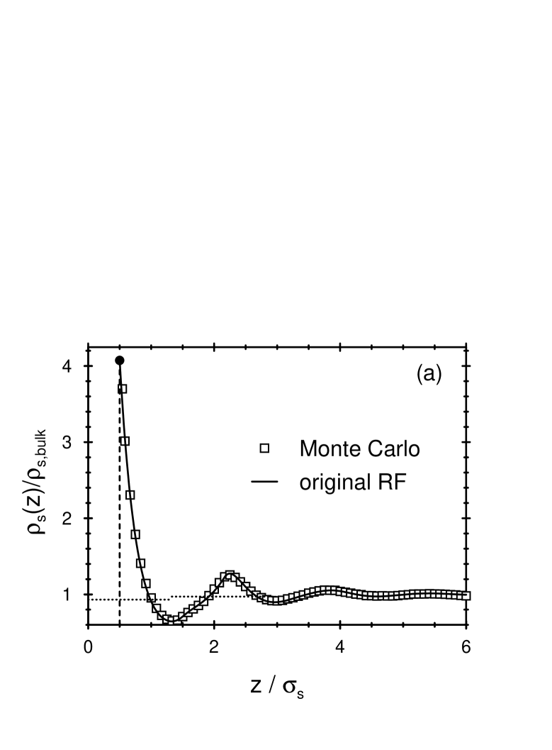
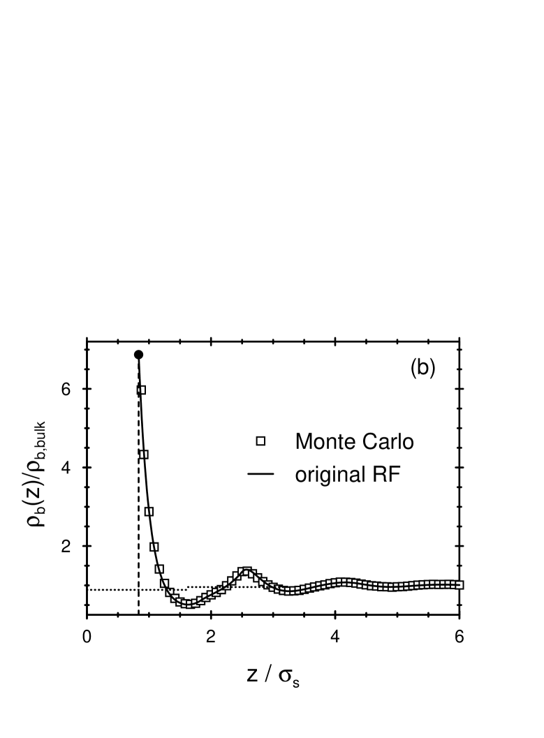
FIG. 1.: The density profiles of the small spheres (a) and the big spheres (b) of a binary hard-sphere mixture with size ratio $R_{b}:R_{s}=5:3$ and packing fractions $\eta_{s}=0.0607$ and $\eta_{b}=0.3105$ close to a planar hard wall (dashed line). $\sigma_{s}=2R_{s}$ is the diameter of the small spheres. The solid lines correspond to results obtained by a free minimization of the original Rosenfeld functional and the symbols ($\square$) denote simulation data from Ref. [10]. The full dots indicate the values at contact. The positions of the extrema of $\rho_{s}(z)$ and $\rho_{b}(z)$ are very close to each other if they are measured from the corresponding position of contact, i.e., $z=R_{s}=\frac{1}{2}\sigma_{s}$ and $z=R_{b}=\frac{5}{6}\sigma_{s}$, respectively. The dotted lines correspond to the coarse grained density profiles defined in Eq. (23). They indicate that in spite of the high contact values the wall actually leads to a slight net depletion for both species in the first layer.

FIG. 2.: The concentration profiles $\Phi_{s}(z)$ and $\Phi_{b}(z)$ of the small spheres and big spheres, respectively, corresponding to the density profiles in Fig. 1. For geometric reasons $\rho_{i}(z\leq R_{i})=0$ with $R_{s}=\frac{1}{2}\sigma_{s}$ and $R_{b}=\frac{5}{6}\sigma_{b}$. Therefore $\Phi_{s}$ and $\Phi_{b}$ are defined only for $z\geq\sigma_{s}$ and $\Phi_{b}(R_{s}<z<R_{b})=0$ and $\Phi_{b}(R_{s}<z<R_{b})=1$.

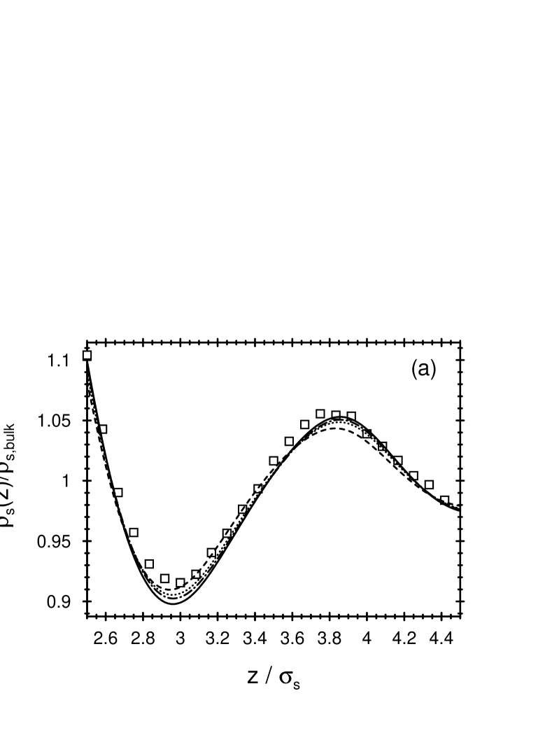
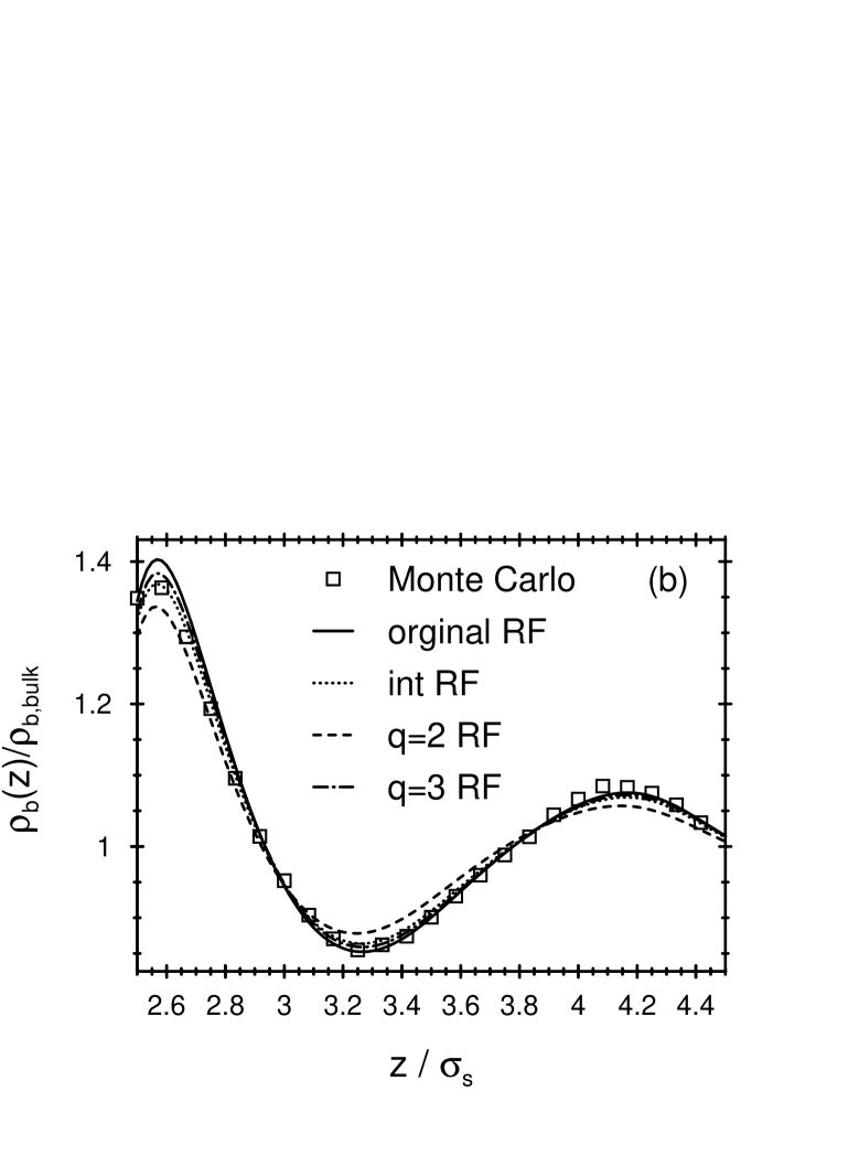
FIG. 3.: In order to resolve the small differences in the density profiles of the small (a) and big (b) spheres between the DFT results obtained by the various versions of the Rosenfeld functional, parts of the density profiles shown in Fig. 1 are magnified here. The solid lines correspond to the original functional, whereas the dotted, dashed, and dashed-dotted lines correspond the interpolated version (int RF), and the antisymmetrized modification with $q=2$ and $q=3$, respectively. The parameters are the same as in Fig. 1.

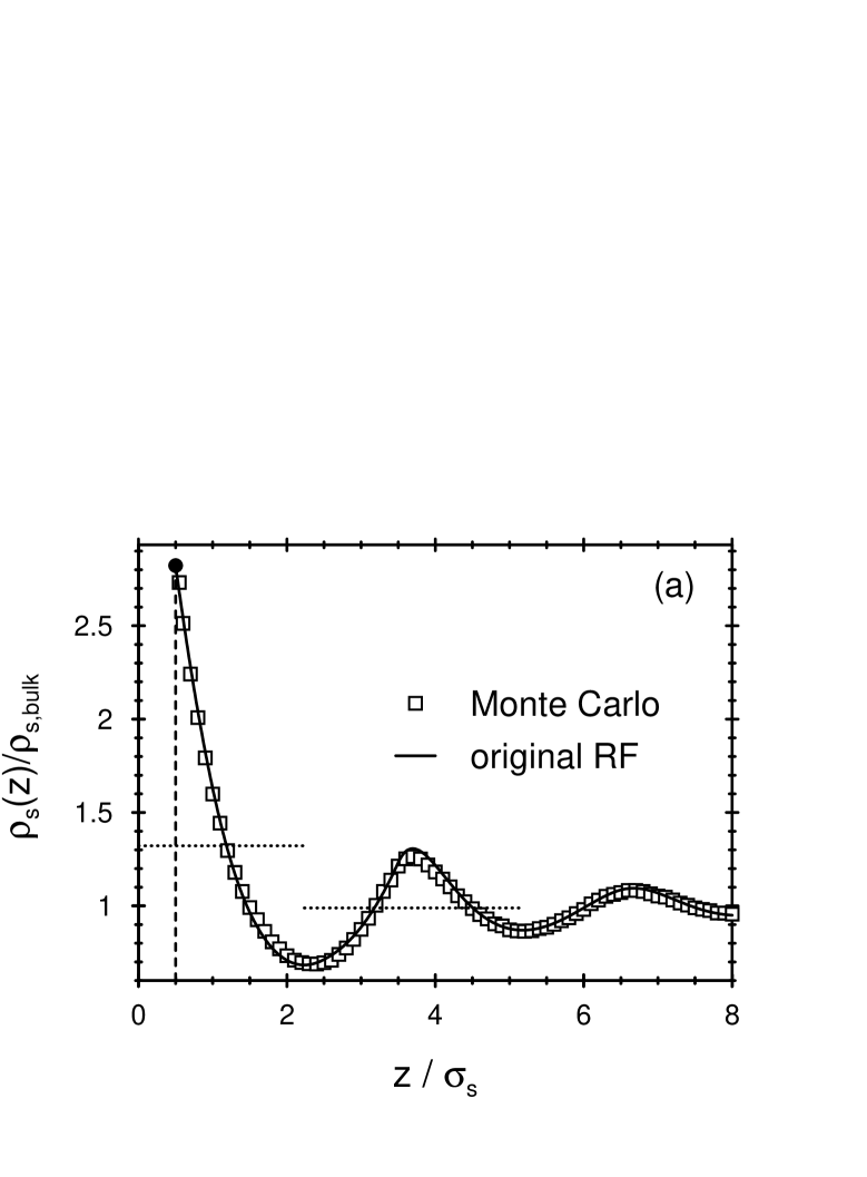
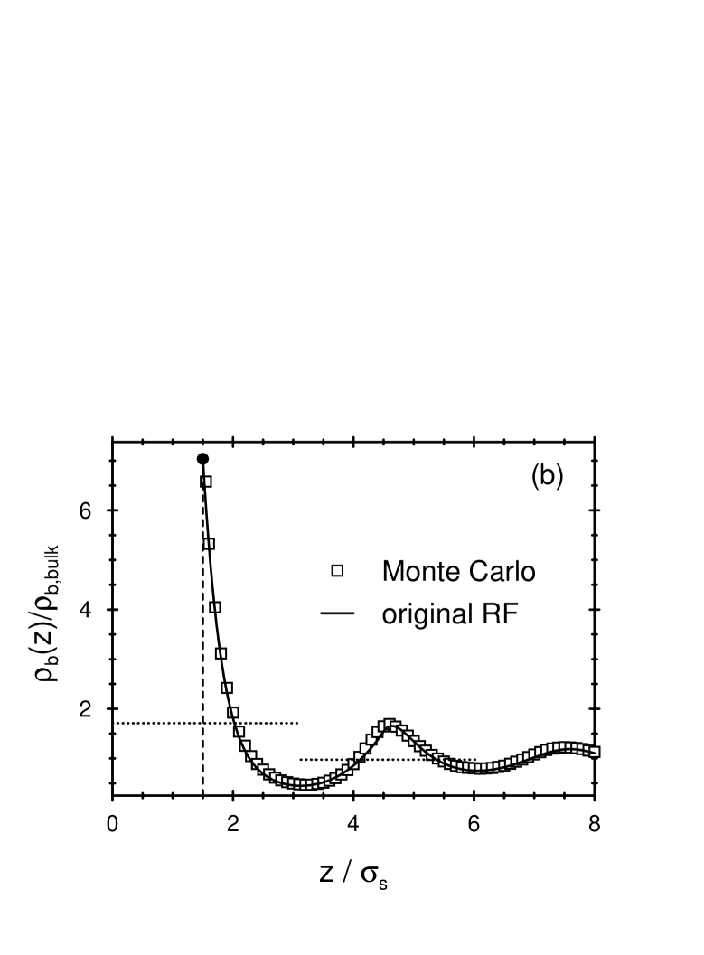
FIG. 4.: The density profiles of the small spheres (a) and of the big spheres (b) of a binary hard-sphere mixture with size ratio $R_{b}:R_{s}=3:1$ and packing fractions $\eta_{s}=0.0047$ and $\eta_{b}=0.3859$ close to a planar hard wall. The solid lines correspond to results obtained by a free minimization of the original Rosenfeld functional. The simulation data ($\square$) are taken from Ref. [10]. As in Fig. 1 the positions of the extrema of $\rho_{s}(z)$ and $\rho_{b}(z)$ are very close to each other if they are measured from the corresponding position of contact, i.e., $z=R_{s}=\frac{1}{2}\sigma_{s}$ and $z=R_{b}=\frac{3}{2}\sigma_{s}$, respectively. The dotted lines correspond to the coarse grained density profiles defined in Eq. (23). Different from Fig. 1, here the net density of both species is clearly enhanced near the wall.

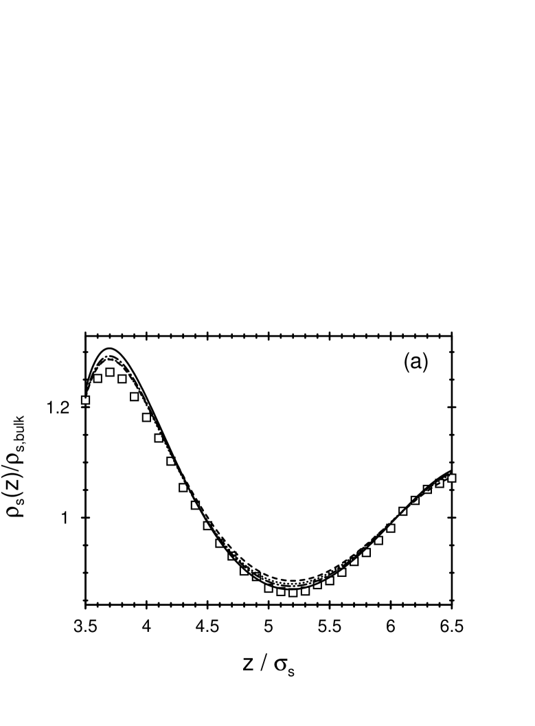
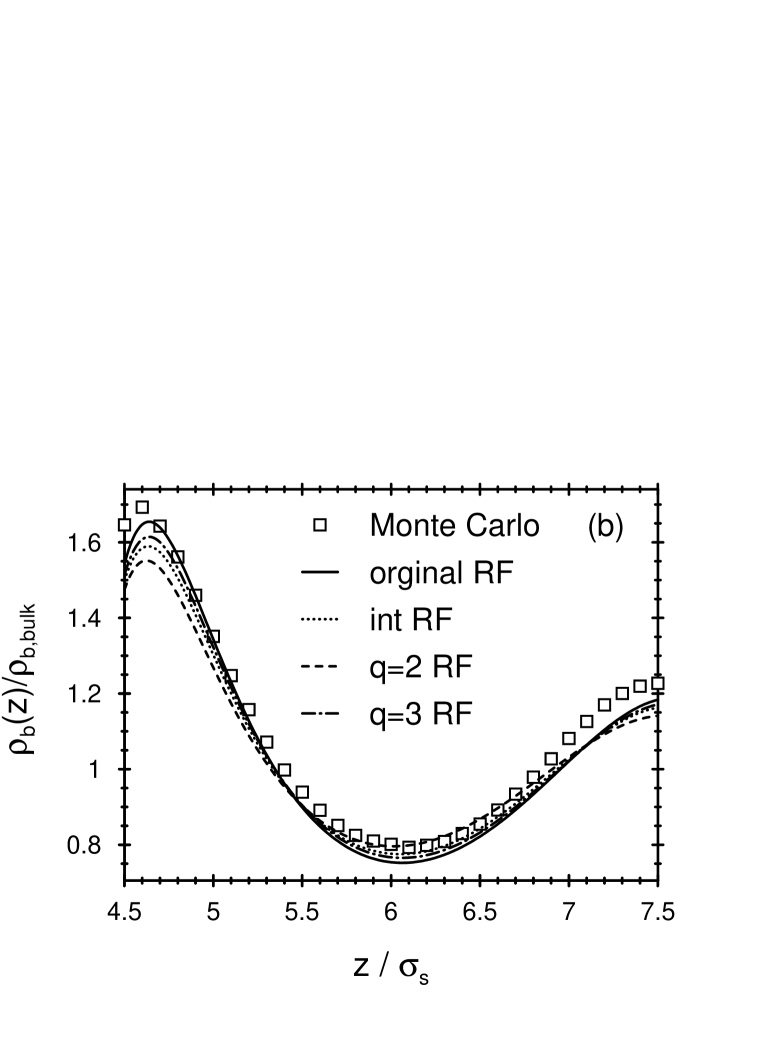
FIG. 5.: In order to highlight the small differences of the DFT results obtained by different versions of the Rosenfeld functional, here small parts of the density profiles shown in Fig. 4 are magnified.

FIG. 6.: The concentration profiles $\Phi_{s}(z)$ and $\Phi_{b}(z)$ of the small spheres and big spheres, respectively, corresponding to the density profiles of Fig. 4. $R_{s}=\frac{1}{2}\sigma_{s}$ and $R_{b}=\frac{3}{2}\sigma_{s}$ so that due to geometric constraints $\Phi_{b}(R_{s}<z<R_{b})=0$ and $\Phi_{s}(R_{s}<z<R_{b})=1$. The anti-correlated behavior of the two profiles is strongly locked in.

FIG. 7.: The excess adsorption $\Gamma_{s}$ of the small spheres near a planar hard wall as function of the packing fractions $\eta_{s}$ and $\eta_{b}$ in the fluid phase [36]. The dots ($\bullet$) denote turning points.

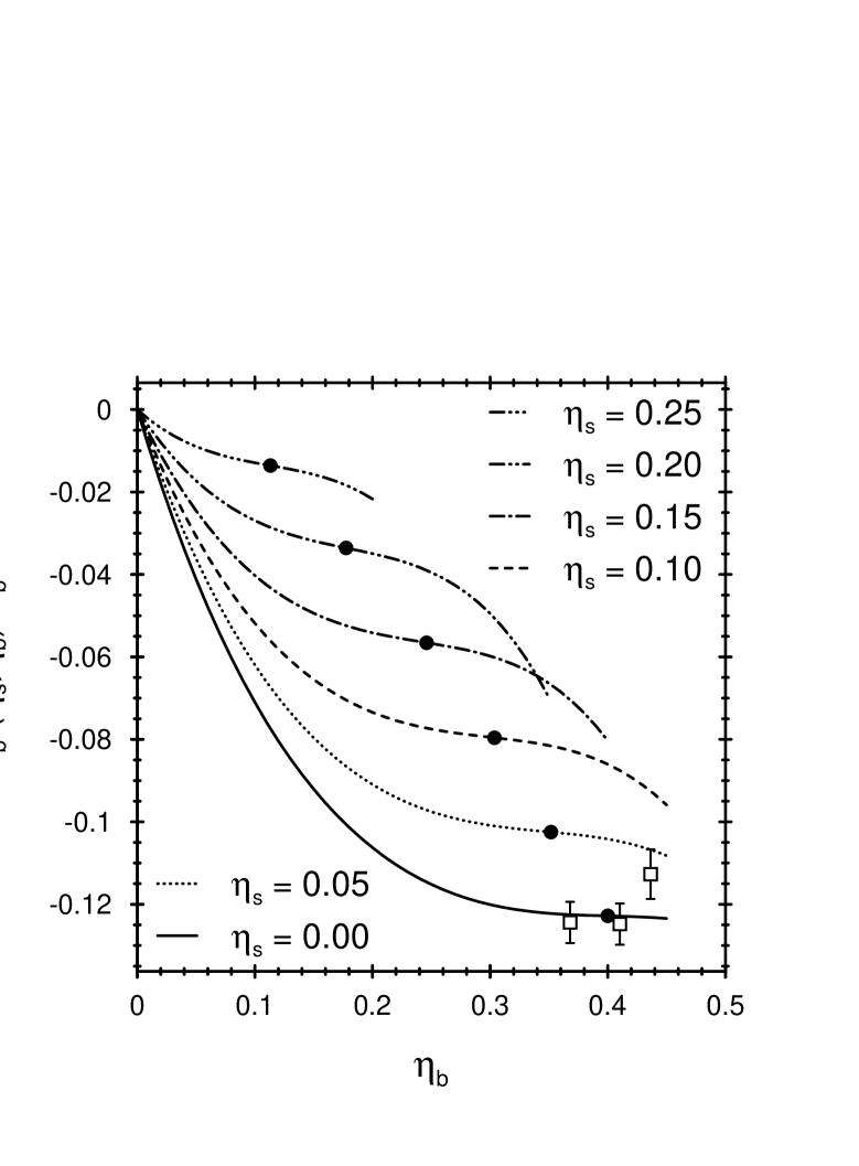
FIG. 8.: The excess adsorption $\Gamma_{b}$ of the big spheres near a planar hard wall as function of the packing fractions $\eta_{s}$ and $\eta_{b}$ in the fluid phase [36]. The dots ($\bullet$) denote turning points. The square symbols ($\square$) denote simulation results for the excess adsorption of a one-component hard-sphere fluid taken from Ref. [35].

FIG. 9.: Excess adsorptions $\Gamma_{s}$ and $\Gamma_{b}$ calculated with the original Rosenfeld functional compared with those obtained from its modification corresponding to Eq. (8). The packing fraction of the small spheres is $\eta_{s}=0.15$.

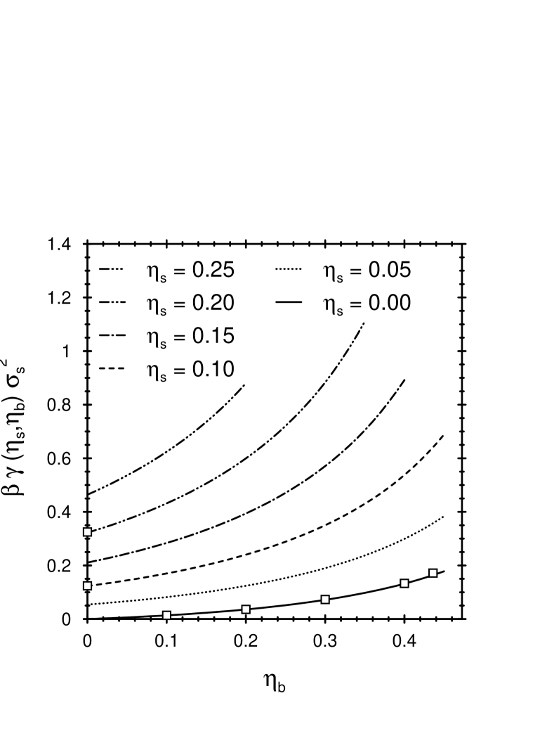
FIG. 10.: The surface tension $\beta\gamma(\eta_{s},\eta_{b})$ of a binary hard-sphere mixture in the fluid phase [36] with size ratio $R_{b}:R_{s}=3:1$ as function of the packing fractions $\eta_{s}$ and $\eta_{b}$, calculated from the original Rosenfeld functional (lines). For $\eta_{s}$=0 the hard-sphere fluid freezes at $\eta_{b}$=0.494. The square symbols ($\square$) denote simulation results from Ref. [38] for the one-component hard-sphere fluid.

TABLE I.: Contact values at a planar hard wall of a binary hard-sphere mixture with size ratio $R_{b}:R_{s}=5:3$ for various packing fractions $\eta_{s}$ and $\eta_{b}$. The comparison of the sum of the contact values with the Percus-Yevick compressibility equation of state, which underlies the Rosenfeld functional, tests the accuracy of our numerical procedures. For small total packing fractions $\eta=\eta_{s}+\eta_{b}$ this equation of state is in good agreement with the more accurate equation of state $\beta p_{MCSL}$ established by Mansoori et al. [31]. However, for larger values of $\eta$, there are deviations.

$\eta$	$\eta_{s}$	$\eta_{b}$	$\sum_{i}\rho_{i}(R_{i}+0)$	$\beta p_{PY}^{c}$	$\beta p_{MCSL}$
0.1246	0.0246	0.1000	0.01804	0.01804	0.01801
0.1252	0.0880	0.0372	0.03809	0.03809	0.03805
0.1309	0.0026	0.1283	0.01256	0.01256	0.01253
0.1850	0.0990	0.0890	0.06116	0.06116	0.06089
0.2005	0.0356	0.1649	0.03901	0.03901	0.03877
0.2247	0.0126	0.2121	0.03697	0.03698	0.03670
0.2278	0.1812	0.0466	0.12304	0.12306	0.12202
0.2670	0.1953	0.0717	0.16351	0.16354	0.16132
0.2749	0.0545	0.2204	0.07985	0.07987	0.07878
0.3477	0.0257	0.3220	0.11401	0.11405	0.11097
0.3712	0.0607	0.3105	0.16908	0.16916	0.16372
0.3906	0.0058	0.2984	0.06845	0.06847	0.06713
0.3968	0.0120	0.3848	0.15642	0.15652	0.15018

TABLE II.: Results for the same quantities as in Table I for a binary hard-sphere mixture with size ratio $R_{b}:R_{s}=3:1$.

$\eta$	$\eta_{s}$	$\eta_{b}$	$\sum_{i}\rho_{i}(R_{i}+0)$	$\beta p_{PY}^{c}$	$\beta p_{MCSL}$
0.1209	0.0188	0.1021	0.00778	0.00778	0.00776
0.1288	0.0037	0.1251	0.00313	0.00313	0.00313
0.1456	0.0283	0.1173	0.01219	0.01219	0.01219
0.2230	0.0026	0.2204	0.00643	0.00643	0.00637
0.2471	0.0199	0.2272	0.01590	0.01590	0.01578
0.2513	0.0089	0.2424	0.01104	0.01104	0.01094
0.3021	0.0016	0.3005	0.01180	0.01180	0.01159
0.3257	0.0136	0.3121	0.02166	0.02166	0.02124
0.3775	0.0099	0.3676	0.02837	0.02837	0.02747
0.3906	0.0047	0.3859	0.02718	0.02719	0.02620

TABLE III.: Individual contact values of the density profiles for a binary mixture with size ratio $R_{b}:R_{s}=5:3$ as obtained by the original Rosenfeld functional ($\sigma_{i}^{3}\rho_{i}^{org}(z=R_{i}+0)$), the antisymmetrized modification with $q=3$ ($\sigma_{i}^{3}\rho_{i}^{q=3}(z=R_{i}+0)$), and the interpolating modification ($\sigma_{i}^{3}\rho_{i}^{int}(z=R_{i}+0)$) with $i=s,b$. $\sigma_{i}=2R_{i}$ is the diameter of species $i$. While all versions of the functional respect the sum rule in Eq. (20), the individual contact values differ slightly for the different versions of the DFT. $\eta=\eta_{s}+\eta_{b}$ is the total packing fraction.

$\eta$	$\sigma_{s}^{3}\rho_{s}^{org}(R_{s}+)$	$\sigma_{s}^{3}\rho_{s}^{q=3}(R_{s}+)$	$\sigma_{s}^{3}\rho_{s}^{int}(R_{s}+)$	$\sigma_{b}^{3}\rho_{b}^{org}(R_{b}+)$	$\sigma_{b}^{3}\rho_{b}^{q=3}(R_{b}+)$	$\sigma_{b}^{3}\rho_{b}^{int}(R_{b}+)$
0.1246	0.07051	0.07058	0.07059	0.34182	0.34150	0.34144
0.1252	0.27332	0.27340	0.27343	0.14522	0.14487	0.14478
0.1309	0.00745	0.00746	0.00746	0.43082	0.43077	0.43077
0.1850	0.38587	0.38639	0.38657	0.47860	0.47619	0.47550
0.2005	0.13385	0.13432	0.13444	0.82502	0.82284	0.82229
0.2247	0.05002	0.05036	0.05043	1.13782	1.13628	1.13594
0.2278	0.90612	0.90702	0.90727	0.36210	0.35787	0.35677
0.2670	1.15640	1.15871	1.15943	0.70205	0.69099	0.68829
0.2749	0.27715	0.27944	0.28026	1.67448	1.66398	1.65994
0.3477	0.17094	0.17520	0.17709	3.43107	3.41124	3.40174
0.3712	0.47247	0.48279	0.48746	4.07483	4.02673	4.00460
0.3906	0.03099	0.03160	0.03181	2.39204	2.38927	2.38826
0.3968	0.10016	0.10471	0.10703	5.33002	5.30870	5.29677

TABLE IV.: Results for the same quantities as in Table I for a binary mixture with size ratio $R_{b}:R_{s}=3:1$.

$\eta$	$\sigma_{s}^{3}\rho_{s}^{org}(R_{s}+)$	$\sigma_{s}^{3}\rho_{s}^{q=3}(R_{s}+)$	$\sigma_{s}^{3}\rho_{s}^{int}(R_{s}+)$	$\sigma_{b}^{3}\rho_{b}^{org}(R_{b}+)$	$\sigma_{b}^{3}\rho_{b}^{q=3}(R_{b}+)$	$\sigma_{b}^{3}\rho_{b}^{int}(R_{b}+)$
0.1209	0.04862	0.04864	0.04864	0.36808	0.36769	0.36761
0.1288	0.00932	0.00933	0.00932	0.42401	0.42387	0.42389
0.1456	0.07891	0.07895	0.07895	0.50360	0.50248	0.50231
0.2230	0.00839	0.00842	0.00841	1.16319	1.16241	1.16248
0.2471	0.07074	0.07101	0.07104	1.52497	1.51744	1.51686
0.2513	0.03121	0.03136	0.03136	1.54220	1.53814	1.53814
0.3021	0.00626	0.00633	0.00633	2.37903	2.37714	2.37714
0.3257	0.05996	0.06072	0.06078	3.05954	3.03862	3.03744
0.3775	0.05168	0.05289	0.05299	4.73342	4.69975	4.69719
0.3906	0.02540	0.02612	0.02617	5.18598	5.16579	5.16450

REFERENCES

- [1] P.N. Pusey, in Liquids, Freezing and the Glass Transition, edited by J.-P. Hansen, D. Levesque, and J. Zinn-Justin (Elsevier, Amsterdam, 1991) p. 763; W. Poon, P. Pusey, and H. Lekkerkerker, Physics World 9, 27 (1996).
- [2] J.-P. Hansen and I.R. McDonald, Theory of Simple Liquids, 2nd ed. (Academic, London, 1986).
- [3] R. Evans, Adv. Phys. 28, 143 (1979); R. Evans, in Fundamentals of Inhomogeneous Fluids (Dekker, New York, 1992); H. Löwen, Phys. Rep. 237, 249 (1994).
- [4] Y. Rosenfeld, Phys. Rev. Lett. 63, 980 (1989).
- [5] R.D. Groot, N.M. Faber, and J.P. van der Eerden, Mol. Phys. 62, 861 (1987).
- [6] I. Pagonabarraga, M.E. Cates, and G.J. Ackland, Phys. Rev. Lett. 84, 911 (2000).
- [7] Z. Tan, U.M.B. Marconi, F. van Swol, and K.E. Gubbins, J. Chem. Phys. 90, 3704 (1989).
- [8] M. Moradi and G. Rickayzen, Mol. Phys. 66, 143 (1989).
- [9] S. Sokołowski and J. Fischer, Mol. Phys. 70, 1097 (1990).
- [10] J.P. Noworyta, D. Henderson, S. Sokołowski, and K.-Y. Chan, Mol. Phys. 95, 415 (1998).
- [11] A.R. Denton and N.W. Ashcroft, Phys. Rev. A 44, 8242 (1991).
- [12] R. Leidl and H. Wagner, J. Chem. Phys. 98, 4142 (1993)
- [13] C.N. Patra, J. Chem. Phys., 111, 6573 (1999).
- [14] N. Choudhury and S.K. Ghosh, J. Chem. Phys. 110, 8628 (1999).
- [15] S.-C. Kim, C.H. Lee, and B.S. Seong, Phys. Rev. E 60, 3413 (1999).
- [16] S.-C. Kim, S.-H. Suh, and C.H. Lee, J. Korean Phys. Soc. 35, 350 (1999).
- [17] Y. Rosenfeld, M. Schmidt, H. Löwen, and P. Tarazona, J. Phys.: Condens. Matter 8, L577 (1996).
- [18] Y. Rosenfeld, M. Schmidt, H. Löwen, and P. Tarazona, Phys. Rev. E 55, 4245 (1997).
- [19] Y. Rosenfeld, in New Approaches to Problems in Liquid State Theory, edited by C. Caccamo, J.-P. Hansen, and G. Stell (Kluwer, Dordrecht, 1999), p. 303.
- [20] Y. Rosenfeld, J. Chem. Phys. 98, 8126 (1993).
- [21] E. Kierlik and M.L. Rosinberg, Phys. Rev. A 42, 3382 (1990).
- [22] S. Phan, E. Kierlik, M.L. Rosinberg, B. Bildstein, and G. Kahl, Phys. Rev. E 48, 618 (1993).
- [23] R. Evans, R.J.F. Leote de Carvalho, J.R. Henderson, and D.C. Hoyle, J. Chem. Phys. 100, 591 (1994).
- [24] J.L. Lebowitz and J.S. Rowlinson, J. Chem. Phys. 41, 133 (1964).
- [25] G. Rickayzen, Mol. Phys. 55, 161 (1985).
- [26] F. van Swol and J.R. Henderson, Phys. Rev. A 40, 2567 (1989).
- [27] With () we denote the packing fraction of the species in the reservoir.
- [28] For the density profiles in Fig. 1 we find the following values: , and , for the small spheres and , and and for the big spheres.
- [29] For the density profiles in Fig. 4 we find the following values: , and , for the small spheres and , and and for the big spheres.
- [30] B. Götzelmann, R. Evans, and S. Dietrich, Phys. Rev. E 57, 6785 (1998).
- [31] G.A. Mansoori, N.F. Carnahan, K.E. Starling, and T.W. Leland Jr., J. Chem. Phys. 54, 1523 (1971).
- [32] N.F. Carnahan and K.E. Starling, J. Chem. Phys. 51, 635 (1969).
- [33] M. Dijkstra, R. Van Roij, and R. Evans, Phys. Rev. Lett. 81, 2268 (1998); ibid 82, 117 (1999); Phys. Rev. E 59, 5744 (1999).
- [34] B. Götzelmann, A. Haase, and S. Dietrich, Phys. Rev. E 53, 3456 (1996).
- [35] J.R. Henderson and F. van Swol, Mol. Phys. 51, 991 (1984).
- [36] The precise phase boundaries towards freezing of a binary hard-sphere mixture with size ratio are not known. Therefore we roughly estimated the onset of freezing from the phase diagram of a binary hard-sphere mixture with size ratio [33] to be close to for , for , for , and for .
- [37] H. Reiss, H.L. Frisch, E. Helfand, and J.L. Lebowitz, J. Chem. Phys. 32, 119 (1960).
- [38] M. Heni and H. Löwen, Phys. Rev. E 60, 7057 (1999).
- [39] D. Henderson and M. Plischke, Proc. Roy. Soc. A 410, 409 (1987).