Absorbing-state phase transitions in fixed-energy sandpiles

Abstract

We study sandpile models as closed systems, with conserved energy density $\zeta$ playing the role of an external parameter. The critical energy density, $\zeta_{c}$, marks a nonequilibrium phase transition between active and absorbing states. Several fixed-energy sandpiles are studied in extensive simulations of stationary and transient properties, as well as the dynamics of roughening in an interface-height representation. Our primary goal is to identify the universality classes of such models, in hopes of assessing the validity of two recently proposed approaches to sandpiles: a phenomenological continuum Langevin description with absorbing states, and a mapping to driven interface dynamics in random media. Our results strongly suggest that there are at least three distinct universality classes for sandpiles.

I INTRODUCTION

Sandpile models [1] are one of the simplest examples of avalanche dynamics, a phenomenon of growing experimental and theoretical interest. In these models, grains of “energy” (sand) are injected into the system, while open boundaries [1] allow the system to reach a stationary state, in which energy inflow (a kind of external drive) and outflow (dissipation) balance. In the limit of infinitely small external driving, the system displays a highly fluctuating, scale-invariant avalanche-like response: the hallmark of criticality.

Ten years after the introduction of the first sandpile automaton by Bak, Tang and Wiesenfeld (BTW)[1], our understanding of its critical behavior remains frustratingly limited, although several variants of the original model have been studied intensively [2, 3, 4, 5]. Despite some remarkable exact results [6, 7], and various renormalization group analyses [8, 9, 10], the tempting possibility of assigning these models their proper universality classes remains unfulfilled. Theoretical and numerical difficulties have likewise hampered the precise estimation of critical exponents. Only recently was the upper critical dimension $d_{c}=4$ established under some assumptions for the avalanche structure [11].

Originally, sandpile models were proposed as the paradigm of self-organized criticality (SOC)[1], i.e., evolution to a critical state without tuning of parameters. For this reason, sandpile models were considered for a long time to inhabit a different world than that of standard critical phenomena. Later, several authors pointed out that, in fact, the SOC state can be ascribed to the presence of two infinitely separated time scales[12, 13, 14, 15]. The two time scales correspond to the external energy input or driving, and the microscopic evolution (“avalanches”). This time-scale separation (also called slow driving), effectively tunes the system to its critical point. What is the relation between critical states due to infinite time-scale separation and regular critical points? This question stimulated many theoretical studies aimed at elucidating the links among sandpile automata and models exhibiting nonequilibrium phase transitions, such as systems with absorbing states[16, 17], interfaces in disordered media[18, 19, 20, 21], the voter model[4], and branching processes[23].

In order to make the connections with other nonequilibrium phenomena more firm, and to establish universality classes, precise critical exponent values are needed. Unfortunately, critical exponents governing the deviation from criticality cannot be measured in slowly driven sandpiles, which are posed by definition at their critical point[22]. Thus correspondences between sandpiles and other nonequilibrium phase transitions can be only partial and inconclusive. In order to overcome this conceptual difficulty, a different approach to sandpiles has been recently pursued[16, 17, 24, 25]. It consists in analyzing sandpiles with fixed energy[26], that is, in considering the same microscopic rules that define sandpile dynamics, but without driving and boundary dissipation. In this way the system is closed and thus the total energy is a conserved quantity, fixed by the initial condition, and can be identified as a (temperaturelike) control parameter. The system turns out to be critical only for a particular value of the energy density (equal to that of the stationary, slowly driven sandpile) and it is thus possible to study deviations from criticality. This approach to sandpiles suggests further analogies with systems with absorbing states[27] and interfaces in disordered media [28, 29].

The stationary state of standard sandpile models is reached through the balance between the input and loss processes, identified by the energy addition and dissipation rates $h$ and $\epsilon$, respectively. Critical behavior is observed in the slow driving regime, in which the parameters $h$ and $\epsilon$ are tuned to their critical values ($h\to 0$ and $\epsilon\to 0$, with $h/\epsilon\to 0$)[15, 16]. In this regime, the system jumps among absorbing configurations (in which activity is null) via avalanche-like rearrangements. Evidently, in absence of external driving, any sandpile model can fall into an absorbing configuration. The connection to absorbing state phase transitions is made more clear by defining closed, fixed-energy sandpiles in which $h\equiv 0$ and $\epsilon\equiv 0$, and periodic boundary conditions are imposed. Since the dynamics admits neither input nor loss, the total energy $E$ is conserved, and the energy density $\zeta=E/L^{d}$ is a tuning parameter. In this case, if the energy density $\zeta$ is large enough, the system reaches a stationary state with sustained activity, i.e., it is in the active phase[16, 27]. On the contrary, for small energy values, the system relaxes with probability one into a frozen configuration, i.e., it is in the absorbing phase. Separating these two regimes is a critical point ($\zeta=\zeta_{c}$) with marginal propagation of activity.

Once it is appreciated that fixed-energy sandpiles exhibit a continuous transition to an absorbing state, the existence of a critical stationary state in the corresponding driven dissipative sandpile is easily understood. That is because energy is added only in the absence of activity ($\zeta<\zeta_{c}$) while dissipation occurs only in the presence of activity ($\zeta>\zeta_{c}$). Thus $d\zeta/dt$ is positive for $\zeta<\zeta_{c}$, and vice-versa, leaving $\zeta_{c}$ as the only possible stationary value for the energy density[30]. (The condition that dissipation and hence activity be absent in the subcritical phase makes the absorbing nature of this phase an essential ingredient of SOC.) Since SOC means tuning a system to its critical point by means of an infinitely slow drive, it is natural to try to understand the critical behavior first in the simpler context of a fixed-energy model. But while many examples of absorbing-state phase transitions have been studied in detail in recent years, we will see that characterizing sandpile criticality, even in the fixed-energy formulation, is a nontrivial project.

In this paper we define and study fixed-energy sandpiles (FES) with various microscopic dynamics. In particular we analyze the BTW sandpile [1], the stochastic Manna model[2, 31], and a model with random mixing of a (real-valued) energy: the shuffling model [32] (full definitions are given in the following section). We show that all of these models exhibit an absorbing-state phase transition at a critical value $\zeta_{c}$ of the energy density. What distinguishes the sandpile from other models with absorbing states is that the control parameter $\zeta$ represents the global value of a conserved field. This phase transition is the basis of the critical behavior of driven self-organized sandpiles. The transition is also studied using mean-field approximations, which yield good qualitative predictions for the order parameter and transition points.

Using the insights provided by the connection with absorbing states, we discuss in detail the attempt to construct a field theory for sandpiles[17]. The latter is a generalization of Reggeon field theory (RFT)[33], the minimal continuum theory describing absorbing-state phase transitions[34]. We also discuss an alternative approach that considers sandpiles from the perspective of linear interface models (LIM) in disordered media[18, 19, 20]. Since continuum descriptions have proved to be of fundamental importance in understanding universality and critical behavior, we analyze in detail open questions and possible improvements of these theoretical approaches.

For all the models mentioned, we report results of simulations close to the critical point, and discuss them in terms of universality classes. Numerical results indicate three distinct critical behaviors, depending upon the microscopic dynamics of models. In particular, the BTW model defines a critical behavior per se, related to the deterministic nature of the dynamics. We find striking evidence of non-ergodicity in the BTW FES: an anomalous transient to the stationary state, and lack of self-averaging. Stochastic automata, such as the Manna model, have a critical behavior that is rather close to the one of linear interface depinning models. Finally, the shuffling model shows a critical behavior that could be compatible with the RFT universality class. However, the nonlocal dynamics of this model merits a detailed examination. It is also important to note that all models show a violation of certain scaling relations usually associated with absorbing-state phase transitions. This seems to point out the particular role of the conserved field in these systems. Finally, we discuss the numerical results in the perspective of the theoretical frameworks mentioned above.

The outline of this paper is as follows: after defining the models in Sec. II, we discuss the generalized RFT theory (Sec. III) and LIM approach (Sec. IV) to FES models. We analyze from a critical perspective the approximations and hypotheses involved in these approaches. In particular, we discuss the nature of the different noise terms; this turns out to be essential to the identification of universality classes. In Sec. V we present the results of extensive simulations in two dimensions, and analyze them in the perspective of absorbing-state transitions [16, 17], and the LIM mapping, which focuses on the roughness of a suitably defined interface [18, 19, 20]. We find differences between BTW, Manna and fully stochastic FES exponents that persist upon enlarging the system size. Sec. VI is concerned with the origins of these differences and possible improvements in the theoretical descriptions to capture the true critical behavior of FES models. A brief summary is provided in Sec. VII. Mean-field theory approaches at the one- and two-site levels are described in the Appendix.

II Fixed-energy sandpiles

In this paper we consider three different sandpile models. All are defined on a $d$-dimensional hypercubic lattice ($d=2$ in this study); the configuration is specified by giving the energy, $z_{i}$, at each site. The energy may take integer or real values, depending on the model, but is nonnegative in all cases. The specific models are defined as follows.

BTW model [1]: Each active site, i.e., with (integer) energy greater than or equal to the activity threshold $z_{th}$ ($z_{i}\geq z_{th}=2d$), topples at unit rate, i.e., $z_{i}\rightarrow z_{i}-z_{th}$, and $z_{j}\rightarrow z_{j}+1$ at each of the $2d$ nearest neighbors of $i$. The toppling rate is introduced in order to define a Markov process with finite transition rates between configurations that differ at a small number of sites. The next site to topple is selected at random from the set of active sites; this is the only stochastic element in the dynamics. (The initial configuration is, in general, random as well.) The BTW dynamics with parallel updating (all active sites topple at each update) is completely deterministic, and it has been possible to obtain many exact results for the driven sandpile in this case, due to the Abelian property[6]. This property implies that the order in which active sites are updated is irrelevant in the generation of the final (inactive) configuration. Accordingly, it is reasonable to expect that sequential or parallel updating does not affect the qualitative behavior. The BTW model is the prototypical sandpile model, and has been the subject of extensive numerical studies [35, 36, 37]. Despite the huge numerical effort devoted to the analysis of its critical behavior, the model presents scaling anomalies which have precluded a definitive characterization. The scattered numerical values of the avalanche critical exponents were recently interpreted in terms of multiscaling properties [38].

Manna sandpile [2, 31]: In this case $z_{th}=2$ regardless of the number of dimensions; the energy is again integer-valued. The two particles liberated when the site $i$ topples move independently to randomly chosen nearest neighbors $j$ and $j^{\prime}$ (That is, $j=j^{\prime}$ with probability $1/2d$) [39]. This model has a stochastic dynamics, which still enjoys a “stochastic” Abelian property, as shown recently by Dhar [31]. The Manna model has also been the subject of many numerical studies. Together with the BTW model, it has been at the center of the long debate over universality classes for (driven) sandpiles [40, 41, 42], that we will discuss in later sections. The Manna model, fortunately, has a regular scaling behavior. The most recent analyses provide a coherent picture of its critical properties and exponent values[41, 42, 43, 44].

Shuffling model[32] : This model has nonnegative real-valued energies. When a site $i$ topples, the energy $Z=z_{i}+\sum_{jNNi}z_{j}$ at that site and its nearest neighbors is redistributed randomly amongst these five sites. That is, we generate random numbers $\eta_{1},...\eta_{5}$, uniform on [0,1], and let $z_{j}\rightarrow z^{\prime}_{j}=\eta_{j}Z/(\eta_{1}+\cdots+\eta_{5})$ ($j=1,...,5$). Sites with energy $z^{\prime}_{j}\geq z_{th}=2$ topple with probability one. In addition, the nearest neighbors of the toppling site that have energy $z^{\prime}_{j}<z_{th}$ also become active with probability $z^{\prime}_{j}/z_{th}$. This model contains stochasticity in each ingredient of the dynamics, and for this reason can be considered a fully stochastic model. It is clearly non-Abelian: the final configuration depends dramatically upon the order in which sites are updated. The parallel-updating version studied in this work exhibits an interesting nonlocal dynamical effect. At each update, the energy around a site is shuffled among nearest-neighbor sites. If a nearest-neighbor (or next-nearest neighbor) pair of sites are both active, the energy at a certain site or sites will be shuffled twice within a single time step. For larger aggregates of active sites, the reshuffling may involve the same site several times. In particular, energy can be transported over large distances by consecutive shuffling events along the front of active sites. This non-locality will create a mixing effect in the energy transport that one expects to influence the critical behavior.

In the present paper, we study the Manna and shuffling models with the parallel updating customarily used in sandpile automata. The BTW model is implemented using random sequential dynamics, with each active site having a toppling rate of unity. The next site to topple is chosen at random from a list of active sites, which must naturally be updated following each toppling event. The time increment associated with each such event is $\Delta t=1/N_{A}$, where $N_{A}$ is the number of active sites. This is the mean waiting-time to the next event, if we were to choose sites blindly, instead of using a list. (In this way, $N_{A}$ sites topple per unit time, just as in a simultaneously updated version of the model.) Since the BTW model is Abelian, the choice of updating (parallel versus sequential) should be irrelevant to the asymptotic critical properties. This has been tested in independent simulations using parallel dynamics[45].

In a FES, the energy density $\zeta$ is fixed in the initial condition. The latter is generated by distributing $\zeta L^{d}$ particles randomly among the $L^{d}$ sites, yielding an initial (product) distribution that is spatially homogeneous and uncorrelated. Once the particles have been placed the dynamics begins. The condition to have at least one active site in the initial configuration is trivially satisfied on large lattices, for the $\zeta$ values of interest, i.e., close to the critical value. (For large $L$, the initial height at a given site is essentially a Poisson random variable, and the probability of having no active sites is exponentially decreasing with the lattice size). It is worth remarking that while the initial conditions are statistically homogeneous, the energy density is not perfectly smooth. For $1\ll l\ll L$, the energy density on a set of $l^{d}$ sites is essentially a Gaussian random variable with mean $\zeta$ and variance $\sim l^{-d}$. The initial value of the critical-site density $\rho_{c}$ (sites that become active upon receiving energy), moreover, is generally far from its stationary value, complicating relaxation to the steady state.

If after some time the system falls into a configuration with no active sites, the dynamics is permanently frozen, i.e., the system has reached an absorbing configuration. We shall see that as we vary $\zeta$, fixed-energy sandpiles show a phase transition separating an absorbing phase (in which the system always encounters an absorbing configuration), from an active phase possessing sustained activity [46]. This is a continuous phase transition, at which the system shows critical behavior. The order parameter is the stationary average density of active sites $\rho_{a}$, which equals zero for $\zeta<\zeta_{c}$, and follows a power law, $\rho_{a}\sim(\zeta-\zeta_{c})^{\beta}$, for $\zeta>\zeta_{c}$. The correlation length $\xi$ and relaxation time $\tau$ both diverge as $\zeta\to\zeta_{c}$; their critical behavior is characterized by the exponents $\nu_{\perp}$ and $\nu_{\parallel}$, defined via $\xi\sim|\zeta-\zeta_{c}|^{-\nu_{\perp}}$ and $\tau\sim|\zeta-\zeta_{c}|^{-\nu_{\parallel}}$, respectively. The dynamical critical exponent is defined via $\tau\sim\xi^{z}$, which implies $z=\nu_{\parallel}/\nu_{\perp}$. The exponents $\beta$, $\nu_{\perp}$ and $\nu_{\parallel}$ define the stationary critical behavior at the absorbing-state phase transition [27]. In the vicinity of the critical point, where $\xi$ is very large, the actual characteristic length of the system is the lattice size $L$. We shall see that the application of finite-size scaling allows us to locate the critical point as well as estimate critical exponents.

III Sandpiles as systems with absorbing states

In this section we discuss a recently proposed phenomenological field theory of sandpiles [17]. Our main goal is to clarify the connection between fixed-energy sandpiles and Reggeon field theory (RFT), which is the minimal field theory describing absorbing-state phase transitions[33, 34] (whose prototypical examples are directed percolation (DP)[47] and contact processes (CP)[48]).

In Ref. [17] we proposed a Langevin description for sandpiles by considering the mean-field description of sandpiles reported in Ref.[15, 16], and introducing spatial dependence and fluctuations. This allows a derivation that is based on the microscopic dynamics of sandpile automata, but involves several approximations.

Here we show how to write down a general Langevin description of sandpiles by using very general symmetry considerations. This results in a complete description, but one that is not easy to deal with, unless the proper approximations are introduced. After the introduction of some specific assumptions regarding noise terms, we recover the results of Ref. [17]. On the other hand, the present more general treatment indicates possible modifications that may be needed for a complete characterization of sandpile models.

In sandpiles, the order parameter is $\rho_{a}$, the density of active sites (i.e., whose height $z\geq z_{c}$) [15, 16, 26]; if at a given time $\rho_{a}({\bf x})=0$ for all x, the system has reached an absorbing configuration. The only dynamics in the model is due the field $\rho_{a}({\bf x})$, which is coupled to the local energy density, $\zeta({\bf x},t)$, which enhances or depresses the generation of new active sites[49]. We therefore consider the dynamics of the local order-parameter field $\rho_{a}({\bf x},t)$ in a coarse-grained description, bearing in mind that the energy density $\zeta({\bf x},t)$ is a conserved field. Note that both $\rho_{a}({\bf x},t)$ and $\zeta({\bf x},t)$ are nonnegative. The most general dynamical equation that imposes local conservation of energy is

$$\frac{\partial\zeta({\bf x},t)}{\partial t}=\nabla^{2}(f_{\zeta}[\{\rho_{a}\},\{\zeta\}])+\nabla\cdot[g_{\zeta}(\{\rho_{a}\},\{\zeta\})\overrightarrow{\eta}({\bf x},t)],$$ (1)

where $f_{\zeta}$ and $g_{\zeta}$ are functionals of $\rho_{a}$ and $\zeta$. Conservation is enforced by the $\nabla^{2}$ term and the standard form of conserving noise, as for example in Cahn-Hilliard-type equations [50] ($\overrightarrow{\eta}$ is a $d$-component vectorial noise). The dynamical equation for the density of active sites can be written analogously as

$$\frac{\partial\rho_{a}({\bf x},t)}{\partial t}=f_{a}(\{\rho_{a}\},\{\zeta\})+g_{a}(\{\rho_{a}\},\{\zeta\})\eta({\bf x},t),$$ (2)

where $f_{a}$ and $g_{a}$ are functionals of $\rho_{a}$ and $\zeta$ and $\eta({\bf x},t)$ is an uncorrelated Gaussian noise. We note that $\eta$ is a nonconserved noise: the active-site density is not a conserved quantity. The functionals $f_{a}$ and $f_{\zeta}$, and variances $g^{2}_{a}$ and $g^{2}_{\zeta}$ appearing on the r.h.s. of Eqs. (1) and (2) are analytic functions (polynomials) of the local densities and (in principle) their spatial derivatives.

The right-hand-sides of Eq.s (1) and (2) must vanish when $\rho_{a}=0$ (if they did not, the state $\rho_{a}=0$ would not be absorbing!). This implies that none of the functionals $f_{a}$, $g^{2}_{a}$, $f_{\zeta}$, and $g^{2}_{\zeta}$ contain terms independent of $\rho_{a}$; they are functions of $\rho_{a}({\bf x},t)$ and the product $\zeta({\bf x},t)\rho_{a}({\bf x},t)$[27]. In this way activity is sustained only if $\rho_{a}({\bf x},t)>0$. It is convenient at this point to introduce a reference value $\zeta_{0}$ of $\zeta$ (for instance the global average energy), and expand the term $\propto\zeta\rho_{a}$ about $\zeta_{0}$. Introducing $\Delta\zeta({\bf x},t)\equiv\zeta({\bf x},t)-\zeta_{0}$ we can express all the functionals as functions of $\Delta\zeta({\bf x},t)\rho_{a}({\bf x},t)$, where all terms of the form $\zeta_{0}[\rho_{a}({\bf x},t)]^{n}$ are absorbed into the coefficient of $[\rho_{a}({\bf x},t)]^{n}$, $\zeta_{0}$ being constant.

In order to write the various functionals more explicitly, we have to consider the symmetry of the lattice in question. For isotropic models the system is inversion-symmetric under ${\bf x}\to-{\bf x}$, so that odd powers of gradients, such as $\nabla\rho_{a}$, are forbidden. This leaves us with functionals such as

$$f_{a}(\{\rho_{a}\},\{\zeta\})=D_{a}\nabla^{2}\rho_{a}({\bf x},t)-r\rho_{a}({\bf x},t)+\mu\rho_{a}({\bf x},t)\Delta\zeta({\bf x},t)-b\rho_{a}^{2}({\bf x},t)+.~{}.~{}.~{}.$$ (3)

where $D_{a},r,\mu$ and $b$ are constants whose connection with the microscopic dynamics will be clarified below. The functionals $f_{\zeta}$, $g_{a}$ and $g_{\zeta}$ have similar forms. If we do not want to deal with an infinite set of power and derivative terms in $\rho_{a}({\bf x},t)$ and $\Delta\zeta({\bf x},t)$, we have to identify the relevant terms from the renormalization group point of view. This can be done via power counting analysis at the upper critical dimension. This implies the knowledge of the noise term, i.e., we have to decide the terms to retain in $g_{a}$ and $g_{\zeta}$. The most relevant term is the linear one, corresponding to $g_{a}\sim g_{\zeta}\sim\rho_{a}^{1/2}({\bf x},t)$ [33, 27]. In RFT, the rationale for the noise variance being proportional to the local order parameter is that the numbers of elementary (birth and death) events in a given space-time cell are Poissonian random variables, so the variance is equal to the expected value. That the noise term for sandpile models has the same form as in RFT is by no means guaranteed. For instance, the BTW model is fully deterministic, and the nontrivial assumption that at the coarse-grained level it is described by a time-dependent noise should be tested. Further, the fact that the field $\zeta({\bf x},t)$ is conserved could affect the noise form. In fact, it is well known that additional symmetries on the fields can change the noise form[51]. In the absence of an exact derivation of the noise terms, we proceed by showing the Langevin description resulting from the choice of a RFT-like noise.

Assuming RFT-like noise terms, the activity equation takes the form

$$\frac{\partial\rho_{a}({\bf x},t)}{\partial t} = D_{a}\nabla^{2}\rho_{a}({\bf x},t)-r\rho_{a}({\bf x},t)-b\rho_{a}^{2}({\bf x},t)$$ (4)

$$+ \mu\rho_{a}({\bf x},t)\Delta\zeta({\bf x},t)+\eta_{a}({\bf x},t),$$ (5)

where $\eta_{a}=\rho_{a}^{1/2}\eta$. Here we have retained only relevant terms with respect to the noise considered. In mean-field theory the critical point corresponds to $r=r_{c}=0$; we expect fluctuations to renormalize $r_{c}$ to a nonzero value. In any case, the value of $r$ depends on $\zeta_{0}$, i.e., the energy density $\zeta_{0}$ plays the role of a (temperaturelike) control parameter.

The evolution of $\Delta\zeta({\bf x},t)$ is governed only by the most relevant term in the functional $f_{\zeta}$, that is, the one linear in $\rho_{a}$. The equation may be integrated formally to yield

$$\Delta\zeta({\bf x},t)=\Delta\zeta({\bf x},0)+\int_{0}^{t}dt^{\prime}\left[D_{\zeta}\nabla^{2}\rho_{a}({\bf x},t^{\prime})+\nabla\cdot\left(\sqrt{\rho_{a}({\bf x},t^{\prime})}{\overrightarrow{\eta}}\right)\right].$$ (6)

Substituting this into Eq. (5) and disregarding irrelevant higher order terms, the proposed Langevin equation for fixed-energy sandpiles becomes [17]:

$$\frac{\partial\rho_{a}({\bf x},t)}{\partial t} = D_{a}\nabla^{2}\rho_{a}({\bf x},t)-r({\bf x})\rho_{a}({\bf x},t)-b\rho_{a}^{2}({\bf x},t)$$ (7)

$$+ w\rho_{a}({\bf x},t)\int_{0}^{t}dt^{\prime}\nabla^{2}\rho_{a}({\bf x},t^{\prime})+\sqrt{\rho_{a}}\eta({\bf x},t).$$ (8)

$\eta$ is a Gaussian white noise whose only non-vanishing cumulants are $\langle\eta({\bf x},t)\eta({\bf x^{\prime}},t^{\prime})\rangle=D\delta({\bf x-x^{\prime}})\delta(t-t^{\prime})$, $c,b$ and $w$ are fixed parameters, and the coefficient of the linear term,

$$r({\bf x})=r-\mu\Delta\zeta({\bf x},0),$$ (9)

inherits its spatial dependence from the initial energy distribution $\Delta\zeta({\bf x},0)$. Observe that $b$ has to be positive to ensure stability; $w>0$ follows from the diffusion coefficient $D_{\zeta}>0$. This equation recovers the result obtained in Ref. [17]; we refer the reader interested in a more phenomenological approach to that paper.

We find, by standard power-counting analysis, that the upper critical dimension of this theory is $d_{c}=4$ [52]. Above $d_{c}$, a qualitatively correct mean-field description is obtained by dropping the noise and gradient terms and replacing $\zeta({\bf x},0)$ by the spatially uniform $\zeta=\zeta_{0}$, yielding:

$$\partial_{t}\rho_{a}(t)=-\overline{r}\rho_{a}(t)-\overline{b}\rho_{a}^{2}(t).$$ (10)

The critical point, $\zeta=\zeta_{c}$, corresponds to $\overline{r}=0$. Above $\zeta_{c}$, we have an active stationary state with $\rho_{a}\sim(\zeta-\zeta_{c})^{\beta}$ with $\beta=1$; for $\zeta<\zeta_{c}$, the system falls into an absorbing configuration in which $\rho_{a}=0$. Other MF critical exponents can be calculated as well.

The present Langevin equation resembles RFT, except for the spatial dependence of $r$ and the non-Markovian term. Both stem from the interaction between activity with the energy background. Let us present here some comments on these two extra terms.

Quenched disorder: in the absence of the memory term, and for generic initial conditions, $\Delta\zeta({\bf x},0)\neq const.$, Eq. (8) is the field theory of directed percolation with quenched disorder. Disorder is known to be a relevant perturbation in DP below $d_{c}=4$ [53, 54, 55, 56, 57]. On the other hand, the memory and spatially-dependent linear terms together represent coupling to the energy density, which is not quenched-in, but relaxes via the diffusion of activity [see Eq. (9)]. Thus the effect of a spatially-dependent $r$, in the present context, is not that of quenched disorder. In fact, we expect the physical effects of quenched disorder, and the present coupling to a conserved energy density (frozen only in the absence of activity), to be quite different[58]. A handwaving argument to justify this assertion is the following: In the active stationary state, close to the critical point, activity will tend to be localized at any given moment, and a given point x will experience bursts of activity interspersed amongst dormant intervals. As activity alternately enters and vanishes from the neighborhood of x, the positive and negative contributions to the Laplacian memory term in Eq. (8) will largely cancel, and so this term will be dominated by the most recent changes in the state of the region. Thus the initial spatial variation in $r({\bf x},0)$ will effectively be forgotten in the stationary state. Another way to see this is to note that the effects of quenched disorder are found in a non-Markovian version of the contact process [57, 59] (using the so-called “run-time statistics”) in which the creation rate at site $i$ is $\lambda_{i}(t)=(c_{i}+a)/(n_{i}+a+1)$, where $a$ is a parameter, and $c_{i}$ represents the number of creation events out of $n_{i}$ total events at site $i$, up to time $t$. Evidently, sites which by chance have enjoyed a larger fraction of creation events in the past are likely to continue to do so, mimicking a quenched random creation rate. In the present case, the effective creation rate ($\propto-r(x)$) is $\lambda(x,t)=\lambda(x,0)+w\int_{0}^{t}dt^{\prime}\nabla^{2}\rho_{a}(x,t^{\prime})$. Now, regions with $\rho_{a}$ larger than $<\rho_{a}>$ tend to have $\nabla^{2}\rho_{a}<0$. Thus the non-Markovian term provides a stabilizing, negative feedback on the creation rate. Regions currently experiencing above-average activity will be harder to excite in the near future. (Note however, that $\int r(x,t)dx$ is time independent, since $\int\nabla^{2}\rho_{a}dx=0$.) While the non-Markovian term effectively erases the initial distribution $r(x,0)$, we do expect the spatial dependence of $r$ to play an important role when we consider avalanches, i.e., the spread of activity from a localized seed, in a nonuniform energy density.

Non-Markovian term: As we have just discussed, this term enables the theory to forget the quenched, stochastic reproduction rate $r({\bf x},0)$. Naively, its associated coefficient, $w$, has the same dimensionality as $b$ and $D$, which are the two marginal parameters of RFT at its upper critical dimension, $d_{c}=4$. Below $d_{c}$ we expect the critical fixed point to be renormalized to $r=r^{*}$, defining a renormalized $\zeta_{c}$ and nontrivial critical exponents. If the non-Markovian term is irrelevant, the field theory would be governed at criticality by the RFT fixed point. In $d=2$ the RFT critical behavior is characterized by $\beta\simeq 0.58$, $\nu_{\perp}\simeq 0.73$ and $z\simeq 1.77$[27]. We shall see in the following sections that numerical results are not compatible with this picture in the BTW and Manna case. This calls for a full RG analysis of Eq. (8). Unfortunately, this is a very dificult task because of primitive divergencies appearing in the perturbative approaches. A discussion of the RG treatment of the present field theory will be reported elsewhere[52].

Possible modifications and generalizations of Eq. (8), and their implications for critical behavior, will be discussed in later sections. Finally, a microscopic derivation of the field theory would ensure that the conservation symmetry has been properly taken into account in the present phenomenological approach.

IV Sandpiles as interfaces in random media

A connection between sandpiles and interfaces moving in disordered media can be obtained by defining a variable $H(i,t)$ that counts the number of topplings (instances of activity) at site $i$ up to time $t$. This variable defines a growing surface in a $d+1$ dimensional space. The interface is said to be in the pinned phase if its disorder-average velocity $<\!\partial_{t}H(i,t)\!>$ is null; a finite velocity marks the moving phase. It is then easy to recognize that the pinned phase in interface models is completely analogous to an absorbing state, while the moving phase corresponds to an active state [60]. To make this correspondence more precise let us note that a nonzero interface velocity is only possible if active sites are present in the system; equivalently we can notice that $\partial_{t}H(i,t)=\rho_{a}(i,t)$, so in either representation the dynamically active phase is restricted to the regime with nonvanishing $\rho_{a}(x,t)$. In this way it is evident that pinned (unpinned) and absorbing (active) states are just two ways of looking at the same physical situation. The connection between driven sandpiles and interfaces was first proposed by Narayan and Middleton and by Paczuski and Boettcher [18, 19] and recently generalized by Lauritsen and Alava [20, 21] who provided a direct mapping between the BTW model and a linear interface with quenched disorder. In the following we adapt their approach to fixed-energy sandpiles.

Let $H_{i}(t)$ be the number of topplings at site $i$ up to time $t$, and $z_{i}(t)$ the energy at $i$ at time $t$. The latter is evidently the difference between the inflow and the outflow of energy at site $i$ in the past. The outflow is given by $2dH_{i}(t)$, since in each toppling $2d$ particles are expelled from the site. There are two contributions to the inflow, the first being the energy $z_{i}(0)$ present at time $t=0$. The second comes from topplings of the nearest-neighbor sites, and can be expressed as $\sum_{NN}H_{j}(t)$. Summing the above contributions we obtain:

$$z_{i}(t) = z_{i}(0)+\sum_{jNNi}H_{j}(t)-2dH_{i}(t)$$ (11)

$$= z_{i}(0)+\nabla_{D}^{2}H_{i}(t),$$ (12)

where $\nabla_{D}^{2}$ stands for the discretized Laplacian.

Since sites with $z_{i}(t)>z_{c}=2d-1$ topple at unit rate, the dynamics of the height follows

$$\frac{dH_{i}(t)}{dt}=\Theta[z_{i}(0)+\nabla_{D}^{2}H_{i}(t)-z_{c}],$$ (13)

where $dH_{i}(t)/dt$ is a shorthand notation for the rate at which the integer-valued variable $H_{i}(t)$ jumps to $H_{i}(t)+1$, and $\Theta(x)=1$ for $x>0$ and is zero otherwise. Since $z_{i}(t)$ takes integer values, the smallest argument of the $\Theta$-function yielding a nonzero toppling rate is unity. If we replace $\Theta(x)$ by $x$, and assume this change to be irrelevant for critical properties [61], then the BTW FES is mapped onto a discretized Edward Wilkinson (EW) equation [28, 62] with quenched disorder, represented by the fluctuations in the $z_{i}(0)$ term. A noise term of this kind, which varies from site to site, but is time-independent, is referred to as columnar noise in the field of interface dynamics [63, 64].

To understand the phenomenology of Eq. (13), let us define the average initial energy as $f=\langle z_{i}(0)\rangle$. There are three different possibilities.

• If $f$ is small then with probability one the system is eventually pinned by disorder.

• If $f$ is large enough, the system has a finite velocity and keeps moving indefinitely.

• Separating these two regimes is a critical point marking the depinning transition.

Thus the phase transition in the BTW FES is analogous to a depinning transition. If the caveat noted above regarding the replacement $\Theta(x)\to x$ turns out to be unimportant, then the transition should show the same scaling properties as depinning in the Edward-Wilkinson equation with columnar noise.

How are these results changed for the Manna model? For the outflow at site $i$ we now have $2H_{i}(t)$, since only two particles are transferred in each toppling event. The total input is the sum of the initial energy, $z_{i}(0)$, and a stochastic contribution $I_{i}(t)$ associated with topplings at the nearest neighbors of $i$:

$$I_{i}(t)=\sum_{jNNi}\sum_{\tau=1}^{H_{j}(t)}\eta_{i,j}(\tau)\;,$$ (14)

where the $\eta_{i,j}(\tau)$ are a set of independent (for $i$ fixed!), identically distributed random variables that specify the number of particles (0, 1, or 2) received by site $i$ at the $\tau$-th toppling of site $j$. Thus

$$\eta_{i,j}(\tau)=\left\{\begin{array}[]{ll}0&\mbox{with probability $(1-1/2d)^{2}$}\\ 1&\mbox{with probability $(1-1/2d)/d$}\\ 2&\mbox{with probability $(1/2d)^{2}$}\end{array}\right.$$ (15)

Of course, the variables associated with different acceptor sites $i$ are highly correlated, since $\sum_{i}\eta_{i,j}(\tau)=2$. $\eta_{i,j}(\tau)$ has mean $1/d$ and variance $(1-1/2d)/d$. It is convenient to introduce $\xi_{i,j}(\tau)\equiv\eta_{i,j}(\tau)-1/d$, which has zero mean, the same variance as $\eta_{i,j}(\tau)$, and obeys $\sum_{i}\xi_{i,j}(\tau)=0$. We may now write the analog of Eq. (12) for the Manna model:

$$z_{i}(t)=z_{i}(0)+\frac{1}{d}\nabla_{D}^{2}H_{i}(t)+\sum_{jNNi}\sum_{\tau=1}^{H_{j}(t)}\xi_{i,j}(\tau).$$ (16)

To obtain a simple EW-like equation for the height in the Manna model, we must (1) ignore the correlations between noise terms associated with different sites, and (2) imagine that the noise is updated when site $i$ itself, rather than one of its neighbors, topples; we will denote the noise term as $\xi_{i}(H)$. Under these assumptions we may write

$$\frac{dH_{i}(t)}{dt}=\left\{\begin{array}[]{ll}1\;,&\mbox{if}\;\;z_{i}(0)+\frac{1}{d}\nabla_{D}^{2}H_{i}(t)+\xi_{i}(H)\geq 2\\ 0\;,&\mbox{ otherwise}.\end{array}\right.$$ (17)

We have obtained an EW-like equation with quenched as well as columnar disorder, the so-called linear interface model. This last equation has been studied extensively both theoretically and numerically[28, 29, 62]. If the previously discussed approximations are irrelevant, the Manna model should belong to the LIM universality class [28, 29]. The fact that the correlations between the noise terms are short range argues in favor of this conclusion [21].

The shuffling model deserves a particular note. In fact, it is not obvious that we can write an exact relation between the (continuous-valued) energy $z_{i}(t)$ and the height (number of topplings) $H_{i}(t)$. It is possible to write an interface equation for the shuffling model if we introduce some phenomenological constants and approximations beyond those used in the Manna case. We do not report the full derivation, which finally leads to an equation of the form of Eq. (17).

We have seen that two issues remain unresolved:

i) Whether the approximations involved in the Manna and shuffling cases change the critical behavior from the LIM universality class.

ii) Whether the various models are in the same universality class, since even if the approximations in i) are irrelevant, the Manna equation involves quenched as well as columnar noise, while only the latter appears in the BTW equation.

In order to answer the above questions analytically, a more rigorous study of the noise terms appearing in the interface equations is needed. This is analogous to the Langevin description of the previous section. We caution however that this analogy does not imply that it is easy, or even possible, to translate equations or results from one language to the other. For example, to the best of our knowledge, no one has succeeded in writing down an interface-like equation equivalent to RFT[65].

From a numerical point of view it is possible to measure various exponents characterizing the behavior of moving interfaces. Many of these exponents can be related to those measured in the context of absorbing-state phase transitions. It appears clear from the previous discussion that the driving force in the interface picture is equivalent to the energy density $\zeta$. This is the control parameter, and the exponents $z$ and $\nu_{\perp}$ are the same in both pictures. Moreover, the order parameter exponent $\beta$ is equivalent to the interface velocity exponent usually measured in interface depinning models. More interestingly, associated with the interface picture are new exponents, related to the interface roughness, defined as :

$$W^{2}(L,t)=\frac{1}{L^{d}}<\sum_{i}(H_{i}(t)-\overline{H(t)})^{2}>$$ (18)

where $\overline{H(t)}=L^{-d}\sum_{i}H_{i}(t)$ and the $<>$ brackets represent an average over different realizations. In general one expects $W^{2}$ to exhibit an $L$-independent, power-law growth regime prior to saturating, that is [62]

$$W^{2}(t,L)\sim\left\{\begin{array}[]{ll}t^{2\beta_{W}}\;,&t\ll t_{\times}\\ L^{2\alpha}\;,&t\gg t_{\times},\end{array}\right.$$ (19)

where the crossover time $t_{\times}\sim L^{z}$. The limiting behaviors described above follow from the dynamic scaling property,

$$W^{2}(t,L)=L^{2\alpha}{\cal W}(t/L^{z})\;,$$ (20)

where the scaling function ${\cal W}(x)\sim x^{2\beta_{W}}$ for small $x$, and attains a constant value for $x\rightarrow\infty$. The dynamic exponent thus satisfies the scaling relation $z=\alpha/\beta_{W}$ (first proposed by Family and Viseck [66]). We expect a data collapse for different system sizes in a plot of $L^{-2\alpha}W^{2}(t,L)$ versus $t/L^{z}$. The roughness exponents are related via scaling relations to the other critical exponents. One may show, for example, that $\beta_{W}=1-\theta$. To see this, note that in the power-law growth regime, for which the correlation length $\xi(t)\ll L$, growth events in different regions are uncorrelated. Given the scaling property of the single-site height probability, $P[H_{i}(t)]=f[H_{i}(t)/\overline{H(t)}]$, we have $W^{2}(t)={\rm var}[H_{i}(t)]\propto[\overline{H(t)}]^{2}$. Since $\overline{H(t)}$ is simply the integrated activity, $\overline{H(t)}=\int_{0}^{t}dt^{\prime}\rho_{a}(t^{\prime})\propto t^{1-\theta}$, yielding $\beta_{W}=1-\theta$.

At this point it is well to raise a caution regarding the naive application of scaling laws such as those mentioned in the preceding paragraph. Recent numerical studies have revealed that many growth models may exhibit anomalous roughening, i.e., the local width (calculated on ‘windows’ of size $l<<L$) scales with an exponent, $\alpha_{loc}$, other than $\alpha$. In these cases, simple scaling a la Family-Viscek does not hold. Technically this corresponds to the following situation: $W(l,t)\approx t^{\beta_{W}}{\cal F}_{A}(l/t^{1/z})$, with an anomalous scaling function given by:

$${\cal F}_{A}(u)\sim\left\{\begin{array}[]{lcl}u^{\alpha_{loc}}&{\rm if}&u\ll 1\\ {\rm const.}&{\rm if}&u\gg 1\end{array}\right.,$$ (21)

it is only for $\alpha_{loc}=\alpha$ that usual self-affine scaling [66] is recovered. This phenomenon has recently been elucidated by López (see [67] and references therein). In general it originates from an additional correlation length, shorter than the system size, that enters as a relevant parameter in scaling equations, destroying self-affinity. In practical terms, it is important to observe that in the presence of anomalous roughening, if due attention is not paid (i.e., if scaling relations are naively assumed to hold), one can measure different correlation-time exponents depending on the type of experiment one performs. Let us finally point out that the linear interface model, at least in $d=1$, exhibits anomalous roughening [68], and therefore some of the scaling anomalies we observe could be ascribed to effects of this nature. This is an issue that certainly deserves further study.

V Simulation results

In this section we present numerical simulations of FES models. All three FES models studied here exhibit a critical point; for large enough values of $\zeta$ the active site density (in the infinite-size limit) has a nonzero stationary value. In order to study the critical point and the scaling behavior of the active state in simulations of finite systems, we must study the quasistationary state that describes the statistical properties of surviving trials. The finite system size $L$, in fact, introduces a correlation length so that even above the critical point some initial configurations lead to an absorbing state. In practice, we compute average properties over a set of $N_{samp}$ independent trials, each using a different initial configuration ($N_{samp}$ ranges from $10^{3}$ to $10^{5}$ depending on the lattice size). Quasistationary properties are calculated from averages restricted to surviving trials. The active-site density exhibits the usual finite-size rounding in the neighborhood of the transition point; only in the limit $L\to\infty$ does the transition become sharp. For this reason, finite-size scaling is a fundamental tool in the location of the critical point as well as the calculation of critical exponents [70].

A The Manna FES model

We performed simulations of the Manna fixed-energy sandpile in the version in which the two particles liberated when a site topples move independently to randomly chosen nearest neighbors. We studied lattices ranging from $L=32$ to $1024$ sites on a side, using homogeneous, random initial configurations as described in Sec. II.

After a transient whose duration depends on the system size $L$ and on $\Delta\equiv\zeta-\zeta_{c}$, the surviving sample averages reach a steady value. In Fig. (1) we show how the density of active sites approaches a mean stationary value $\overline{\rho_{a}}(\Delta,L)$. At a continuous transition to an absorbing state, the order parameter ($\rho_{a}$ in this instance) is expected to follow the finite-size scaling form

$$\overline{\rho_{a}}(\Delta,L)=L^{-\beta/\nu_{\perp}}{\cal R}(L^{1/\nu_{\perp}}\Delta)\;,$$ (22)

where ${\cal R}$ is a scaling function with ${\cal R}(x)\sim x^{\beta}$ for large $x$, since for large enough $L>>\xi\sim\Delta^{-\nu_{\perp}}$ we must have $\overline{\rho_{a}}\sim\Delta^{\beta}$. To locate $\zeta_{c}$ we study the stationary active-site density as a function of system size. When $\Delta=0$ we have that $\overline{\rho_{a}}(0,L)\sim L^{-\beta/\nu_{\perp}}$; for $\Delta>0$, by contrast, $\overline{\rho_{a}}$ approaches a stationary value, while for $\Delta<0$ it falls off as $L^{-d}$. Only at the critical point do we obtain a nontrivial power law, which allows us to locate the critical value $\zeta_{c}$. In Fig. 2 we observe power-law scaling for $\zeta=0.71695$, but clearly not for 0.7170 or 0.7169, allowing us to conclude that $\zeta_{c}=0.71695(5)$. (Figures in parenthesis denote statistical uncertainties.) The associated exponent ratio is $\beta/\nu_{\perp}=0.78(2)$.

Next we consider the scaling behavior of the active-site density away from the critical point. The finite-size scaling form of Eq. (22) implies that a plot of $\rho\equiv L^{\beta/\nu_{\perp}}\overline{\rho_{a}}$ versus $x\equiv L^{1/\nu_{\perp}}\Delta$ will show a data collapse for systems of different sizes. In practice, we determine the horizontal and vertical shifts (i.e., in a log-log plot of $\rho_{a}$ versus $\Delta$) required for a data collapse. In Fig. 3, the best data collapse for $L\geq 48$ is obtained with $\beta/\nu_{\perp}=0.78(2)$ and $1/\nu_{\perp}=1.22(2)$. These values correspond to an exponent $\beta=0.64(2)$. This is recovered also by a direct fitting of the scaling function ${\cal R}(x)$ for large $x$ (see Fig. 3). A good estimate of $\beta$ can be also obtained by looking at the scaling of the stationary density with respect to $\Delta$ for the largest possible sizes $L$. In this case if $\Delta>0$ and $L>>\xi$ we have the scaling behavior $\overline{\rho_{a}}\sim\Delta^{\beta}$. In Fig. 4, we show the active site density as a function of $\Delta$ for $L=1024$. The resulting power-law behavior yields $\beta=0.64(1)$, where the error is dominated by the uncertainty in the critical point $\zeta_{c}$.

To determine the dynamical exponent $z=\nu_{||}/\nu_{\perp}$ we study the probability $P(t)$ that a trial has survived up to time $t$. The latter appears to decay, for long times, as $P(t)\sim\exp(-t/\tau_{P})$. At the critical point, the characteristic decay time $\tau_{P}$ is a power-law function of the only characteristic length in the system, the system size $L$. Thus, we have $\tau_{P}(L)\sim L^{z}$ for $\Delta=0$. An estimate of $\tau_{P}(L)$ can be obtained by direct fitting of the exponential tail of $P(t)$, or by the time required for the survival probability to decay to one half. In Fig. 5 we report the behavior of $\tau(L)$ close to the critical point. Power-law behavior is recovered at the critical point, yielding $z=1.57(4)$. (The error bar is again dominated by the uncertainty in the critical value $\zeta_{c}$.) As a further consistency check we considered the density $\rho_{a,all}(t,L)$, that is, the active-site density averaged over all trials, including those that have reached the absorbing state $\rho_{a}=0$. Assuming that the time dependence involves a single characteristic time that scales as $L^{z}$, we write at the critical point $\Delta=0$

$$\rho_{a,all}(t,L)=t^{-\theta}g(tL^{-z})$$ (23)

where $g(x)$ is a constant for $x\ll 1$ and decays faster than any power law for $x\gg 1$. A data collapse can be obtained by plotting $\rho_{all}=\rho_{a,all}(t,L)t^{\theta}$ versus $x=tL^{-z}$. The best data collapse is obtained with $\theta=0.42(1)$ and $z=1.56(3)$; it is shown in Fig. 6. This result confirms that the dynamical exponent is in the range $z\simeq 1.55-1.6$. An exponent $\theta=0.42(1)$ is found also in the decay of the active-site density $\rho_{a}(t)$ averaged only over the surviving trials (see Fig. 1). In simple absorbing-state transitions, the latter exponent is consistent with the usual scaling relation $\theta=\beta/\nu_{||}$, obtained by assuming, for $\Delta=0$, the simple scaling behavior $\rho_{a}(t)=L^{\beta/\nu_{\perp}}y(tL^{z})$, with $y(x)=const$ for $x\to\infty$. In the Manna FES model, this simple scaling behavior is not observed, and the relaxation of the order parameter shows qualitatively different scaling regimes. In particular, $\rho_{a}(t)$ exhibits a sharp drop (which seems to grow steeper with increasing $L$) just before entering the final approach to $\overline{\rho_{a}}$ (see Fig. 1). Accordingly, the exponent $\theta$ violates the usual scaling relation, and it is impossible to obtain a good data collapse with simple scaling forms. This is probably due to the introduction of an additional characteristic length that defines the relaxation to the quasistationary state (we are presently studying the possible relation between this effect and anomalous roughening). Moreover, it is not clear if the choice of initial conditions plays a role in this peculiar behavior. A more detailed study of the relaxation to the stationary state is required in order to understand the origin of these scaling anomalies, which appear in all the sandpile models analyzed in this paper, as well as in the one-dimensional Manna FES [71].

The interface mapping described in Sec. IV prompted us to study the dynamics of the mean width $W(t,L)$ [see Eq.(18)]. We studied the evolution of the width at $\zeta_{c}$, in systems of size $L=128$ to 800. Unfortunately, we were not able to reach the complete saturation regime of the roughness, which would afford an independent estimate of the exponent $\alpha$. This is due to the exponential decay of the survival probability at very large times. As shown in Fig. 7, we obtain a good collapse using the values $\alpha=0.80(3)$ and $z=1.57(2)$. Following Eq. (19), the short-time behavior of $W(t,L)$ gives an exponent $\beta_{W}=0.51(1)$. This exponent, however, shows a systematic increase with the system size $L$. In particular, for large sizes ($L\geq 512$) it seems that a simple power-law regime is not adequate to represent the temporal behavior of the interface width. Note also that the scaling relation $\theta+\beta_{W}=1$, satisfied to within uncertainty for the other models considered, is violated in the Manna case: $\theta+\beta_{W}=0.93(2)$. It appears that some of the anomalies affecting the temporal scaling of surviving trials could be influencing the estimates of the roughness exponents. Also in this case, further studies, for example of the local roughness, are needed for a direct comparison with other interface growth models.

In summary, numerical results show clear evidence of the critical behavior usually observed in absorbing phase transitions. Critical exponents and a discussion about universality classes will be provided in the next section. Finally, we note that the Manna sandpile does not exhibit the strong nonergodic effects reported below for the BTW model.

B The BTW FES model

In Ref. [16] preliminary results on the two-dimensional BTW model were reported; here we present a more detailed study, including considerably larger lattices. To study stationary properties, we performed, for each system size $L$ = 20, 40,…1280, and energy density $\zeta$, $N_{samp}$ independent trials (ranging from $5\times 10^{4}$ for $L=20$ to 1600 for $L=1280$), each extending up to a maximum time $t_{max}$. The latter, which ranged from 800 for $L=20$ to $3\times 10^{5}$ for $L=1280$, was sufficient to probe the stationary state. An overall idea of the dependence of the active-site density on $\zeta$ can be gotten from Fig. 8, which compares simulation results with the pair approximation derived in the Appendix.

The simulations reported in Ref. [16], which extended to systems of linear dimension $L=160$, permitted us to conclude that $\zeta_{c}=2.1250(5)$ [72]. We first discuss the results of simulations performed at $\zeta_{c}$. Figure 9 shows the relaxation of the active- and critical-site densities at $\zeta_{c}$; note the non-monotonic approach to the limiting values. The inset shows that there is a deterministic, linear relation between the two densities during the relaxation process: for $\zeta=\zeta_{c}$, a least-squares fit yields $\rho_{c}=\rho_{c,cr}-C\rho_{a}$, where $C=1.368$ and $\rho_{c,cr}=0.4459$ is the critical site density at $\zeta_{c}$ in the limit $L\rightarrow\infty$ (for which $\rho_{a}$ naturally falls to zero). We note that this relation is independent of system size $L$ and of sample-to-sample variations (for the same $L$); all that changes is the portion of the line filled in by the data. For off-critical values of the energy density, the active- and critical-site densities follow a different linear trend [73].

In Fig. 10 we plot $\overline{\rho_{a}}(\zeta_{c},L)$ and the excess critical-site density $|\overline{\rho_{c}}(\zeta_{c},L)-\zeta_{c,cr}|$ (overbars denote mean stationary values), versus $L$ on log scales, anticipating that these decay $\sim L^{-\beta/\nu_{\perp}}$. The apparent power-law behavior for small $L$ is followed, for larger $L$, by an approach to a larger exponent. For $L\geq 320$ we obtain the estimates of $\beta/\nu_{\perp}=0.78(3)$ and 0.77(2) from the active-site and critical-site density, respectively, but it is clear that the slope of this plot has not stabilized even for $L=1280$.

Next we consider the relaxation time at $\zeta_{c}$. There are two independent quantities whose relaxation is readily monitored: the survival probability $P(t)$ and the active-site density $\rho_{a}(t)$. (Given the strict linear relationship between $\rho_{a}$ and $\rho_{c}$, we cannot treat the latter as an independent dynamical variable; not surprisingly, the two yield essentially the same relaxation times.) We studied four different relaxation times; the first two are associated with the survival probability $P(t)$. This quantity decays slowly at first, then enters a regime of roughly exponential decay, after which it attains a nearly constant value $P_{P}$. (While $P(t)$ appears to decay very slowly after attaining $P_{P}$, the relaxation times we study here are for the approach to $P_{P}$.) We define $\tau_{P}$ as the relaxation time associated with the exponential-decay regime; another relaxation time, $\tau_{\overline{P}}$, is defined as the time at which $P(t)$ equals $(1+P_{P})/2$, midway to its quasi-stationary value. As we have seen, $\rho_{a}(t)$ exhibits a non-monotonic approach to its stationary value, and does not exhibit a clear exponential regime. Taking advantage of the non-monotonicity, we define $\tau_{m}$ as the time at which $\rho_{a}$ takes its minimum value. Finally, we noted that restricting the sample to trials that survive up to $t_{max}$ results in a monotonic, exponential approach to $\overline{\rho_{a}}$ (see Fig. 11 ). A fit to the linear portion of a semi-log plot of the excess density $\rho_{a}(t)-\overline{\rho_{a}}$ yields $\tau_{a}$. Relaxation times in a critical system are expected to diverge with system size as $\tau(\zeta_{c},L)\sim L^{\nu_{||}/\nu_{\perp}}$. The data for all four relaxation times, plotted in Fig. 12, are consistent with a power law, but due to fluctuations, linear fits to the data (for $L\geq 160$) yield exponent ratios ranging from $\nu_{||}/\nu_{\perp}=1.59$ to 1.74. Since the four data sets do seem to follow a common trend, and since there is no reason to expect different relaxation times to be governed by different exponents, we define $\overline{\tau}(L)$ as the geometric mean of all four relaxation times. The behavior of $\overline{\tau}(L)$ is quite regular; linear fits to the data for $L\geq 80$, 160, and 320 yield $\nu_{||}/\nu_{\perp}=1.671$, 1.668 and 1.657, respectively, leading to an estimate of 1.665(20) for this ratio.

Another manifestation of scaling is the short-time decay of the order-parameter density in a critical system, starting from a spatially homogeneous initial configuration [74]. In Fig. 13 we show the active-site density for short-times. The data exhibit an imperfect collapse, and there is no clear-cut power-law regime. The roughly linear region for $L=1280$ yields a decay exponent $\theta\simeq 0.41$.

Next we consider the scaling behavior of the active- and critical-site densities away from the critical point. We analyze these data using the finite-size scaling form of Eq. (22), which implies that a plot of $\tilde{\rho}\equiv L^{\beta/\nu_{\perp}}\overline{\rho_{a}}$ versus $\tilde{\Delta}\equiv L^{1/\nu_{\perp}}\Delta$ will show a data collapse for systems of different sizes. The data analysis is as described above for the Manna FES. The best data collapse (see Fig. 14) for $L\geq 80$ is obtained with $\beta/\nu_{\perp}=0.75(2)$ and $1/\nu_{\perp}=1.15(2)$. (This value of $\beta/\nu_{\perp}$ is slightly smaller than the value obtained above from the scaling of $\rho_{a}$ at $\zeta_{c}$; note however that the latter value, 0.78(3), is based on systems with $L\geq 320$.) ¿From this finite-size scaling analysis we therefore obtain the values $\nu_{\perp}=0.87(2)$ and $\beta=0.65(2)$. One again, though, it is important to check for size dependence of the exponent estimates. Fitting the linear portion of the $\rho_{a}$ data in the scaling plot, we obtain $\beta=0.62$, 0.63, 0.66 and 0.69 for $L=80$, 160, 320 and 640, respectively.

We can apply a similar analysis to the density of critical sites, but here we must isolate the singular part of $\rho_{c}$ from an analytic background. The latter appears because for $\zeta<\zeta_{c}$, $\rho_{c}$ increases smoothly with $\zeta$. Above $\zeta_{c}$, $\rho_{c}$ decreases linearly with $\rho_{a}\sim\Delta^{\beta}$, so we expect the singular part $\rho_{c,sing}=A\Delta^{\beta}$ for $\Delta>0$, with $A<0$. The simplest reasonable form for the nonsingular background is $\rho_{c,reg}=\rho_{c,cr}+B\Delta$, where $\rho_{c,cr}=0.4459$ is the $L\rightarrow\infty$ critical value as noted above. We expect the singular part of $\rho_{c}$ to follow the same finite-size scaling form as the active-site density. This implies that

$$\rho_{c}^{*}(\tilde{\Delta},L)\equiv L^{\beta/\nu_{\perp}}(\rho_{c}-\rho_{c,cr})=-C{\cal R}(\tilde{\Delta})+BL^{(\beta-1)/\nu_{\perp}}\tilde{\Delta}\;.$$ (24)

Thus the singular contributions cancel in $\rho_{c}^{*}(L)-\rho_{c}^{*}(L^{\prime})$. Using the values for $\nu_{\perp}$ and $\beta/\nu_{\perp}$ found in the scaling analysis of $\rho_{a}$, we study $\rho_{c}^{*}(L)-\rho_{c}^{*}(L^{\prime})$ for all pairs of system sizes in the range $L=80,...,640$, and obtain $B=0.71(2)$. We can then construct a scaling plot of the singular part, $\tilde{\rho}_{c,sing}\equiv L^{\beta/\nu_{\perp}}|\rho_{c}-\rho_{c,cr}-B\Delta|$, which shows a fair data collapse (see Fig. 14), but with much more scatter than for $\rho_{a}$, presumably because of the uncertainties involved in isolating the singular contribution. As in the case of the active-site density, the $\beta$ estimates we obtain from the $\rho_{c,sing}$ data increase with $L$. Here we find $\beta=0.65$, 0.65, 0.67 and 0.70 for $L=80$, 160, 320 and 640, respectively. We conclude that $\beta\stackrel{{\scriptstyle>}}{{\sim}}0.7$. Studies of larger lattices will be required to refine this estimate.

We studied the evolution of the interface width $W(t,L)$ as defined in Eq (18), at $\zeta_{c}$, in systems of size $L=20$ to 640, with sample sizes ranging from $5\times 10^{4}$ for $L=20$ to $10^{3}$ for $L=640$. As shown in Fig. 15, we obtain a good collapse for $L\geq 40$ using the values $\alpha=1.01(1)$ and $z=1.63(2)$. The exponent $\alpha$ can be found directly from the data for the saturation value of $W^{2}$ shown in Fig. 16. Fitting the short-time (power-law) data for $W^{2}$ yields an estimate for the growth exponent $\beta_{W}$, which increases systematically with $L$, as shown in the inset of Fig. 16. Extrapolating to infinite $L$ we obtain $\beta_{W}=0.62$, in agreement with the scaling relation $\beta_{W}=\alpha/z$ . Note also that the value of $z$ describing the interface growth crossover time is consistent, as one would expect, with that for $\nu_{||}/\nu_{\perp}$, derived from a study of relaxation times.

The size dependence of the critical exponents could be an indication of the failure of the simple scaling hypothesis [38]. A further anomalous aspect of the BTW FES is nonergodicity: in a particular trial, properties such as $\rho_{a}$ typically differ from the mean value computed over a large number of trials. This means that time averages are different from averages over initial configurations, where the latter play the role of “ensemble averages”. It is worth remarking that this nonergodicity is consistent with the existence of toppling invariants [6]. In Fig. 17, for example, we show the evolution of $\rho_{a}$ for five different initial configurations (ICs) in a system with $L=80$, at $\zeta_{c}$. Each IC appears to yield a particular active-site density; fluctuations about this value are quite restricted, and typically do not embrace the mean over ICs. Fig. 17 also shows histograms of the stationary mean active-site density (for a given IC), in samples of 10⁴ ICs, for $L=80$ and 160; the distribution has a single, well-defined maximum, and narrows with increasing $L$. The data indicate, however, that the probability distribution for $\rho_{a}/\overline{\rho_{a}}$ (i.e., the order parameter normalized to its mean value), does not become sharp as $L\rightarrow\infty$, as it would, for example, in directed percolation.

Further evidence of nonergodicity is found in the activity autocorrelation function, defined as

$$C(t)\equiv\frac{\langle N_{A}(t_{0}+t)N_{A}(t_{0})\rangle}{\langle N_{A}(t_{0})\rangle^{2}}-1,$$ (25)

where $N_{A}(t)$ is the number of active sites at time $t$, and $\langle...\rangle$ stands for an average over times $t_{0}$ in the stationary state for a given IC, as well as an average over different ICs. The autocorrelation function for the critical BTW FES ($L=80$, average over 2000 ICs and $10^{4}$ time units), shown in Fig. 18, exhibits surprisingly little structure. After decaying rapidly to a minimum value at around $t=34$, and increasing to a weak local maximum near $t=62$, $C(t)$ seems to fluctuate randomly about zero. The relaxation occurs on a time scale over an order of magnitude smaller than for $\rho_{a}$ or the survival probability (the relaxation times $\tau_{m}$ and $\tau_{\overline{P}}$ $\approx 800$ for this system size).

The reason for this anomalously rapid decay becomes clear when we examine the autocorrelation function in individual trials ($C(t)$ defined as in Eq. (25) but without averaging over ICs). Figures 19 and 20 show some typical results for $L=80$. (Here, to get good statistics, we have averaged over $5\times 10^{5}$ to $10^{6}$ time units in the stationary state.) The correlation function in a single trial shows shows considerable structure, including damped oscillations (and in some cases, revivals), which may be superimposed on a more-or-less linear decay. The period (in the range 35 - 70 for $L=80$) and other features vary from one IC to another. (Changing the seed for the random choice of toppling sites changes $C(t)$ only slightly, if we maintain the same IC [75].) Evidently, $C(t)$ decays rapidly to zero when we average over initial conditions because of dephasing amongst oscillatory signals with varied frequencies. Interestingly, the interface width $W(t,L)$ shows much less dependence on the IC than does the active-site density or its autocorrelation.

In summary, the BTW fixed-energy sandpile shows signs of the kind of scaling found at simpler absorbing-state phase transitions, but at the same time exhibits dramatic nonergodic effects. We note unusually strong finite-size effects, which prevent us from determining certain critical exponents precisely. Whether this is a simple finite-size effect or a signature of multiscaling cannot be ascertained definitively with the present data.

C The Shuffling FES model

The shuffling model[32] has a continuously variable control parameter, since each site has a (non-negative) real-valued energy. Thus we are no longer constrained to vary the energy density $\zeta$ in increments of $1/L^{2}$ as we are in discrete models (e.g., the Manna and BTW FES), where the single grain is the smallest energy unit. In the shuffling FES, all sites whose energy exceeds the threshold $z_{th}=2$ are considered active. In addition, sites that have received energy from a toppling nearest neighbor can become active if $z_{i}<z_{th}$ with a probability $p_{i}=z_{i}/z_{th}$. This enlarges considerably the choice of possible initial configurations. In particular, after we have distributed randomly the total amount of energy among the lattice sites, we extract for each site a random number $\eta_{i}$ and we declare active all sites for which $\eta_{i}\leq z_{i}/z_{th}$. (Obviously, sites with $z_{i}\geq z_{th}$ are active with probability one.) Unlike discrete models, we have the option of generating “flat” initial conditions, in which all sites have the same energy. While stationary properties are not affected by the choice of noisy versus flat initial configurations, we do note differences in the short-time behavior.

Another peculiar characteristic of the shuffling model is the strong non-Abelian character of its dynamics. We implemented the dynamics of the model with parallel updating as in the original definition of Ref. [32]. However, this form of the dynamics contains some non-local effects as described in Sec. II, and does not ensure that parallel and sequential updating generate the same critical behavior. Simulations with sequential updating are in progress.

Simulations of the shuffling model require many calls to the random number generator, and so are extremely time-consuming. Here we present simulations with flat initial conditions and sizes ranging from $L=32$ to $L=384$. By analyzing the $L$-dependence of $\overline{\rho_{a}}(\Delta,L)$ we find the critical point $\zeta_{c}=0.20427(5)$. When $\zeta=\zeta_{c}$ the stationary density has a power-law behavior $\overline{\rho_{a}}(0,L)\sim L^{\beta/\nu_{\perp}}$ that yields $\beta/\nu_{\perp}=0.76(3)$. This result is confirmed by the scaling plot of Fig. 21, which, following Eq. (22) shows $\rho\equiv L^{\beta/\nu_{\perp}}\overline{\rho_{a}}$ versus $x\equiv L^{1/\nu_{\perp}}\Delta$, with $\beta/\nu_{\perp}=0.76$ and $1/\nu_{\perp}=1.266$. This gives an exponent $\beta=0.60$, as confirmed by the straight slope of the upper branch of the scaling plot. An independent measurement of the stationary density versus $\Delta$ for the largest size used ($L=384$) gives the estimate $\beta=0.60(2)$, where the error bar is due mainly to the uncertainty in $\zeta_{c}$.

We performed a scaling analysis of the temporal behavior by studying the decay of the survival probability $P(t)\sim\exp(-t/\tau_{P})$. At the critical point the $L$-dependence of the characteristic time assumes the power-law behavior $\tau_{P}\sim L^{z}$ with $z=1.71(5)$ (see Fig. 22). However, it is worth noting that the scaling behavior with $L$ shows a systematic curvature from the smallest to the largest sizes, both below and above the critical point. This could be a signal that the system has not yet reached its asymptotic temporal behavior for the sizes considered ($L\leq 320$). That the relaxation could be affected by strong finite-size effects is confirmed by the temporal scaling of $\rho_{a}(t,L)$. In Fig. 23 we observe that the active-site density decay does not follow a definite power law before reaching the stationary state. This makes impossible an accurate determination of the exponent $\theta$ ($\approx 0.46$), which is also reflected in the absence of a clear data collapse for the temporal scaling functions.

The roughness analysis is affected by several numerical problems. The short average lifetime of trials at finite size makes it impossible to reach the width-saturation regime. This effect is even more pronounced than in the Manna case. It is therefore impossible to apply a data-collapse analysis, nor is a direct measurement, that would yield $\alpha$, feasible. The short-time behavior of the roughness (see Eq. (18)) is governed by the exponent $\beta_{W}\simeq 0.57$. Applying the scaling relation shown in Sec. IV, and using the dynamical exponent obtained previously, we have $\alpha\simeq 0.96$. However, in this case the short-time behavior of the roughness appears to have a size dependence, probably due to the lack of complete convergence to the asymptotic scaling behavior, and the numerical values provided here could contain systematic errors that are difficult to estimate.

In summary, the numerical results for the shuffling FES model show also the signature of a continuous phase transition from an absorbing to an active phase. The stationary properties of the model show well defined scaling behavior at the system sizes considered in the present study. The dynamic scaling properties, by contrast, show anomalies and transient effects that could indicate that the system has not yet attained its asymptotic behavior for $L\leq 384$.

VI Discussion and open questions

A Universality classes and critical exponents

Simulations of sandpile models have mainly been performed in the slow driving regime. It is then natural to compare the critical exponents measured in the fixed-energy framework (see Tab. I) with those observed in driven simulations. In driven sandpiles, critical behavior is characterized by the scaling of the number of topplings $s$ and the duration $t$ following the addition of an energy grain[1], i.e., an avalanche. The probability distributions of these variables are usually described with the finite-size scaling forms

$$P(s)=s^{-\tau_{s}}{\cal G}(s/s_{c})$$ (26)

$$P(t)=t^{-\tau_{t}}{\cal H}(t/t_{c})$$ (27)

where $s_{c}\sim L^{D}$ and $t_{c}\sim L^{z}$ are the characteristic avalanche size and time, respectively. Applying the fundamental result (due to conservation), $<s>\sim L^{2}$[6, 15, 26], we can write the scaling relations $\tau_{s}=2-2/D$ and $\tau_{t}=1+(D-2)/z$. Recently, these simple scaling forms have been questioned in the case of the BTW model[38]. An accurate moment analysis seems to show multiscaling, so that scaling relations obtained from the above finite-size scaling forms do not apply.

While critical exponents governing the deviations from criticality in FES do not have any counterpart in the driven case, which is posed by definition at the critical point, the exponents describing the critical point, including $z$ and the fractal dimension $D$, can be compared directly. In FES simulations $D$ can be calculated by noting that the scaling of an avalanche due to a point seed scales as the total variation of the field $H(i,t)$, which represents the total number of topplings. Since the roughness scales with exponent $\alpha$, we readily obtain that $D=d+\alpha$[19, 20].

For the Manna model, our simulations yield $D=2.80(3)$ and $z=1.57(4)$, which should be compared with the most recent analyses of driven sandpiles, which yield $D=2.76(2)$ and $z=1.56(2)$[41, 42, 43, 44]. By using scaling relations we obtain $\tau_{s}\simeq 1.29$ and $\tau_{t}\simeq 1.51$, again in very good agreement with the values obtained in the driven case. For the shuffling model we can compare our results $z=1.71$ and $D=2.96$ with the simulations of Maslov and Zhang[32], which give $z=1.73(5)$ and $D=2.92(5)$. In this case we also see a very good agreement between independent measurements.

More subtle is the case of the BTW model. Here different simulations of the driven sandpile give rather scattered results. A very recent analysis suggesting multiscaling in the (driven) BTW sandpile indicates that neither $D$ nor $z$ are clearly defined[38]. In particular, the effective value of $D$ increases as one studies higher moments, and saturates at $D\simeq 3.0$. This is indeed the result we recover from our analysis ($D=3.01(1)$). The possibility of multiscaling is supported by the scaling anomalies and the lack of self-averaging we detected in our simulations of the BTW FES.

We shall attempt, on the basis of our numerical results, to assign the various fixed-energy sandpiles studied to universality classes. This a particularly vexing problem, that has eluded ten years of theoretical and numerical efforts. Soon after the introduction of sandpile models with modified dynamical rules, there were many quests for the precise identification of universality classes. In particular BTW and Manna models, which are prototypes for deterministic and stochastic models, respectively, have been the objects of a longstanding quarrel over their supposed universality classes[2, 35, 37, 40, 41, 42, 43]. The first numerical attempts showed very similar exponents for the avalanche distributions[2, 35], but the results were afflicted by severe finite-size errors due to the limited sizes attainable using the CPU power available at that time. These results were later questioned by Ben-Hur and Biham[40], who analyzed the scaling of conditional expectation values of various quantities related to avalanches. These results were, however, biased by the unexpected singular behavior of the distributions[41], and have been recently reconsidered by applying other numerical methods [42, 43, 69]. From the theoretical standpoint it is very surprising that small modifications of the microscopic dynamics would lead to different universality class. However, no analytical demonstration of distinct universality classes in sandpiles has been presented up to now. On the contrary, many theoretical arguments in favor of a single universality class can be found in the literature[8].

In Table I we summarize the critical exponents found for each model. The quoted values indicate, beyond numerical uncertainties, that the models discussed here belong to three distinct universality classes. Striking differences appear between the BTW and the Manna model. Beyond the numerical values of critical exponents, we observe for the first time the lack of self-averaging in the BTW FES. This property is related to its deterministic dynamics, and finds consistent analogies in the waves of toppling description[76]. The lack of self-averaging could also be the origin of the multiscaling features recently observed by De Menech et al.[38] in the driven BTW sandpile. From this discussion it appears that the introduction of stochasticity is a relevant modification for the critical behavior. At this point it is worth noting that the Manna model has been considered for a long time as a non-Abelian model. The opposite has been pointed out recently by Dhar[31], by means of rigorous arguments. The conjecture that Manna and BTW sandpiles belong to different universality classes because the former is non-Abelian has then to be abandoned. Stochasticity per se, however, does not define a unique universality class, as evidenced by the distinct critical properties of the Manna and shuffling FES models. The origin of the different behavior can be traced to the nonlocal nature of the shuffling model dynamics, as we shall make clear later.

In summary, our numerical results are in good agreement with the most recent measurements of driven sandpiles, confirming that the two cases share the same critical behavior. In addition, the FES framework enlarges the set of exponents that can be measured, providing new tools for the characterization of critical behavior and universality classes in different models.

B Avalanche and spreading exponents

In order to compare the exponents found in fixed-energy simulations with the usual avalanche exponents $\tau_{s}$ and $\tau_{t}$, we relied on scaling relations. However, avalanches can also be studied in the FES case, in simulations of critical “spreading”. Let us first define what is a spreading experiment in a system with an absorbing-state[27]. In such experiments, a small perturbation (a single active site, for instance) is created in an otherwise frozen (absorbing) configuration. In the supercritical regime, the ensuing activity has a finite probability to survive indefinitely, reaching the stationary state deep inside the (growing) active region. In the subcritical regime, activity will decay exponentially. In each spreading sequence, it is customary to measure the spatially integrated activity $N(t)$, averaged over all runs, and the survival probability $P(t)$ after $t$ time steps. At the critical point separating the supercritical and subcritical regimes, these quantities have a singular scaling: $N(t)\sim t^{\eta}$ and $P(t)\sim t^{-\delta}$, where $\eta$ and $\delta$ are called spreading exponents. If we can define the substrate over which the activity spreads uniquely, this spread of activity is the same as an avalanche in a sandpile model[77].

Sandpile models, however, have infinitely many absorbing configurations. In the infinite-size limit, an infinite number of energy landscapes correspond to the same value $\zeta$. (For real-valued energies, as in the shuffling model, this infinite degeneracy already appears for finite systems.) In this case spreading properties at a given value of the control parameter $\zeta$ will depend on the initial configuration in which the system is prepared. It is even possible to observe nonuniversality in the spreading exponents, a feature that sandpiles share with the pair contact process (PCP)[78, 79] and other systems with infinitely many absorbing configurations[80, 81, 82].

In order to have well defined spreading exponents (that can be related to the avalanche exponents of a driven sandpile), we have to define uniquely the properties of the energy landscape for spreading experiments. One possibility is to use the absorbing configurations generated by the fixed-energy sandpile itself for initial configurations. Suppose we use such a configuration for a spreading experiment, by introducing an active site. Repeating this process many times, we obtain the spreading properties for so-called “natural absorbing configurations”[27]. A second option is to use the substrate left by each spreading process as the initial condition for the subsequent one. After a transient time the system will flow to a stationary state with well defined properties, in which each initial configuration is a “natural configuration”. On the other hand, this second definition of a spreading experiment is identical to slow driving, except that energy is strictly conserved (the active site must be generated by a mechanism that does not change the energy)[24].

By performing spreading experiments close to $\zeta_{c}$, it is possible to obtain directly the avalanche and spreading scaling behavior, as well as the divergence of characteristic lengths approaching the critical energy. A preliminary study in this direction for the BTW model confirms the uniqueness of the critical behavior at $\zeta_{c}$[24]. Interesting results have also been obtained for the spreading properties in a FES mean field model[83]. A more complete study of spreading exponents in a variety of sandpile models is a promising path toward the complete characterization of their critical behavior.

C Comparison with theoretical results

In earlier sections we presented two alternative theoretical descriptions for sandpile models. We compare our numerical results with theoretical predictions in order to assess the validity of these theoretical frameworks, and the eventual improvements needed for a complete description of sandpile models.

In Sec. III we introduced a Langevin description that takes into account the absorbing nature of the phase transition in FES models. Unfortunately, a rigorous derivation of the noise terms has not yet been made. The assumption of RFT-like noise terms leads to the Langevin description of Eq. (8). This differs from the standard DP Langevin description for the presence of a non-Markovian term. Only in the case that this term is irrelevant the theory belongs to the universality class of RFT. From a physical point of view this means that the local coupling between the activity field $\rho_{a}({\bf x},t)$ and the energy field $\zeta({\bf x},t)$ is irrelevant on large scales. In other words the activity spreads on an effective average energy substrate whose only role is to tune the spreading probability. This is indeed the same as a DP problem in which the critical parameter is tuned via the average energy $\zeta$.

Casting a glance at our numerical results, the only model that has exponents compatible with the DP universality class is the shuffling FES. This is not unexpected; the model was indeed proposed by Maslov and Zhang[32] as a sandpile realization of directed percolation. At the basis of this behavior is nonlocal energy transport. As we emphasized in Sec. II, the shuffling model allows the transfer of the same parcel of energy several times in the same time step. This introduces, on average, a strong mixing effect that makes energy diffusion slower. In this way the spread of activity is effectively decoupled from the local fluctuations that the activity itself generates in the energy field. On the other hand, Maslov and Zhang [32] noted that in $d=1$, the nonlocal energy mixing is not capable of destroying correlations and, following a transient, the model exhibits non-DP scaling. While the exponents summarized in Tab. I are compatible with the DP universality class, we note that the dynamic scaling properties of the shuffling model show systematic biases that could signal a nonasymptotic behavior for some observables. We cannot therefore exclude completely that the model is still in a transient regime, that could finally lead to a different critical behavior, as happens in $d=1$.

The Manna and BTW FES models, by contrast, exhibit critical exponents different from those of DP. In these models, the energy redistribution during toppling is strictly local, and the spread of activity is always correlated with the energy fluctuations generated during toppling processes. It is then reasonable to expect that a Langevin theory has to take into account fully the non-Markovian term. It may be also possible to derive the pertinent stochastic equations and the noise correlations applying more rigorous treatments, as in Ref [84].

The moving interface picture is also afflicted by our ignorance of the correlations between the quenched noise terms appearing in the equations (see Sec. IV). By suitable approximations it has been shown that the Manna model could belong to the LIM universality class. Our numerical results show that the stationary critical properties are compatible with this universality class. The dynamic properties, however, show anomalies that are not compatible with LIM. The origin of these anomalies deserves a more accurate analysis, and might be understood if we had a better grasp of the noise terms in the interface representation. It is interesting, in this context, that the BTW model, for which the mapping to the interface representation seems most straightforward, defines a universality class per se, incompatible with linear interface depinning with columnar disorder. This is probably due to the strong nonlinearity introduced by the local velocity constraint implicit in the $\Theta$-function of Eq. (13).

While neither theoretical approach allows an exact characterization of sandpile models, they appear to be conceptually very relevant, because they provide an answer to the basic questions of why driven sandpile models show SOC. The genesis of self-organized criticality in sandpiles is a continuous absorbing-state phase transition. The sandpile exhibiting the latter may be continuous or discrete, deterministic or stochastic. To transform the conventional nonequilibrium phase transition to SOC, we couple the local dynamics of the sandpile to a “drive” (a source with rate $h$). The relevant parameter(s) {$\zeta$} associated with the phase transition are controlled by the drive, in a way that does not make explicit reference to {$\zeta$}. Such a transformation involves slow driving ($h\to 0$), in which the interaction with the environment is contingent on the presence or absence of activity in the system (linked to {$\zeta$} via the absorbing-state phase transition). Viewed in this light, “self-organized criticality” refers neither to spontaneous or parameter-free criticality, nor to self-tuning. It becomes, rather, a useful concept for describing systems that, in isolation, would manifest a phase transition between active and frozen regimes, and that are in fact driven slowly from outside.

A second class of theoretical questions concern the critical behavior (exponents, scaling functions, power-spectra, etc.) of specific models, and whether these can be grouped into universality classes, as for conventional phase transitions both in and out of equilibrium. In this respect, the theoretical approaches presented here show a very promising path of improvements and modifications that could lead to the solution of many of these questions.

VII Summary

We studied three fixed-energy sandpile models, whose local dynamics are those of the BTW, Manna, and shuffling sandpiles, studied heretofore under external driving. The former two models are Abelian, the latter two stochastic. The results of extensive simulations, which are in good agreement (via scaling laws), with previous studies of driven sandpiles, place the three models in distinct universality classes. Results for the Manna FES are consistent with the universality class of linear interface depinning, while the shuffling FES appears to follow directed percolation scaling. Both these assignments, however, are somewhat provisional, due to dynamic anomalies and apparent strong finite-size effects. The case of the BTW FES, which appears to define a new universality class, is further complicated by violations of simple scaling and lack of ergodicity. Examining the field-theoretic and interface-height descriptions of sandpiles in light of our simulation results, we find that a more rigorous description of noise correlations will be required, for these approaches to become reliable predictive tools. Our results strongly suggest that there are at least three distinct universality classes for sandpiles. Whether others can be identified, and how the various classes can be accommodated in a unified field-theoretic description, are challenging issues for future study.

ACKNOWLEDGEMENTS We thank M. Alava and R. Pastor-Satorras for the many results on SOC they have discussed and shared with us prior to publication. We are also indebted with P. Grassberger for comments and private communications. We also acknowledge A. Barrat, A. Chessa, D. Dhar, K.B. Lauritsen, E.Marinari, L. Pietronero and A. Stella for very useful discussions and comments. M.A.M., A.V. and S.Z. acknowledge partial support from the European Network contract ERBFMRXCT980183; M.A.M acknowledges also partial support from the Spanish DGESIC project PB97-0842, and Junta de Andalucía project FQM-165. R.D. acknowledges CNPq and CAPES for support of computing facilities.

TABLE I.: Critical exponents for the FES models studied here compared with known values for DP and the LIM model [28]. Figures in parentheses denote statistical uncertainties.

model	$\beta$	$\beta/\nu_{\perp}$	$z=\nu_{||}/\nu_{\perp}$	$\theta$	$\alpha$	$\beta_{W}$
BTW	$\simeq 0.7$	0.78(3)	1.665(20)	0.41(1)	1.01(1)	0.62(1)
Manna	0.64(1)	0.78(2)	1.57(4)	0.42(1)	0.80(3)	0.51(1)
Shuffling	0.60(2)	0.76(3)	1.71(5)	$\simeq 0.46$	$\simeq 0.96$	$\simeq 0.57$
DP	0.583(4)	0.80(1)	1.766(2)	0.451(1)	0.97(1)	0.55(1)
LIM	0.64(2)	0.80(4)	1.56(6)	0.51(2)	0.75(2)	0.48(1)

Appendix: Mean-Field description

We have devised mean-field approximations for fixed-energy sandpiles at the one- and two-site levels. While the present mean-field theory has nothing useful to say about critical behavior, it is nonetheless interesting that a simple analysis can yield reasonable predictions for the order parameter and transition points. Consider first the one-site approximation for the BTW FES. Let $\rho_{z}$ be the density of sites with energy $z$. Each site receives a unit of energy at rate $n_{a}$, the number of active neighbors. In the one-site approximation the sites are treated as statistically independent, so that in a homogeneous system, the rate of arrival of particles at any site is $2d\rho_{a}$ where $\rho_{a}\equiv\sum_{z\geq 2d}\rho_{z}$ is the density of active sites. In addition to receiving energy, sites with $z\geq z_{th}=2d$ make a transition to $z-z_{th}$ at unit rate. Hence the mean-field equations are

$$\frac{d\rho_{z}}{dt}=2d\rho_{a}(\rho_{z-1}-\rho_{z})+\rho_{z+2d}-\theta_{z\!-\!2d}\;\rho_{z},$$ (28)

where $\theta_{j}=0$ for $j<0$ and is unity otherwise, and $\rho_{-1}$ (in the equation for $z=0$) is of course zero.

This set of equations satisfies probability conservation ($\sum_{z}\rho_{z}$ is constant), and conserves the mean energy $\zeta\equiv\sum_{z}z\rho_{z}$. We try to find a stationary solution by introducing the simplifying assumption that for $z\geq 2d$, the distribution follows an exponential decay:

$$\rho_{z}=\alpha^{z-2d}\rho_{2d},\;\;\;\;\;\;\;\;z\geq 2d.$$ (29)

Under this assumption, the active-site density $\rho_{a}=\rho_{2}/(1-\alpha)$ in one dimension. $\rho_{0}$ can be eliminated using normalization:

$$\rho_{0}=1-\rho_{1}-\frac{\rho_{2}}{1-\alpha}.$$ (30)

Then the mean-field equations become

$$\frac{d\rho_{1}}{dt}=\rho_{2}\left[\alpha+\frac{2}{1-\alpha}\left(1-2\rho_{1}-\frac{\rho_{2}}{1-\alpha}\right)\right]$$ (31)

$$\frac{d\rho_{2}}{dt}=\rho_{2}\left[\alpha^{2}-1+\frac{2}{1-\alpha}(\rho_{1}-\rho_{2})\right]$$ (32)

and

$$\frac{d\rho_{z}}{dt}=\rho_{2}\left[\alpha^{z}-\alpha^{z-2}+\frac{2\rho_{2}}{1-\alpha}(\alpha^{z-3}-\alpha^{z-2})\right]\;,\;\;\;\;\;\;\;\;z\geq 3.$$ (33)

The last equation implies that in the stationary state $\rho_{2}=\frac{\alpha}{2}(1-\alpha^{2})$, and therefore $\rho_{a}=\frac{\alpha}{2}(1+\alpha)$. From Eq. (32) we then have $\rho_{1}=\frac{1}{2}(1-\alpha^{2})$ in the stationary state. Thus $\rho_{2}=\alpha\rho_{1}$ and the distribution is exponential starting with $\rho_{1}$. One readily verifies that the r.h.s. of Eq. (31) is also zero for the stationary values of $\rho_{1}$ and $\rho_{2}$ given above.

The mean energy is given by:

$$\zeta=\rho_{1}+\rho_{2}\sum_{n=0}^{\infty}(n+2)\alpha^{n}=\frac{1}{2}\frac{1+\alpha}{1-\alpha},$$ (34)

so that

$$\alpha=\frac{2\zeta-1}{2\zeta+1},$$ (35)

which shows that the active stationary state exists only for $\zeta>\zeta_{c}=1/2$. Below this value, $\rho_{a}=0$ and $\rho_{1}=\zeta$. (We have also verified that this solution is stable for $\zeta>1/2$.) In the active stationary phase,

$$\rho_{a}=\frac{4\zeta}{(2\zeta+1)^{2}}(\zeta-\zeta_{c}),$$ (36)

so the order parameter exponent $\beta=1$, the usual mean-field value for systems lacking “up-down” symmetry.

The two-dimensional case is only slightly more complicated; the mft equations may be written so:

$$\frac{d\rho_{z}}{dt}=4\rho_{a}(\rho_{z-1}-\rho_{z})-\theta_{z-4}\rho_{z}+\rho_{z+4},$$ (37)

where $\rho_{a}\equiv\sum_{z\geq 4}\rho_{z}$. We now suppose that in the active stationary state, $\rho_{z}=\alpha^{z-4}\rho_{4}$ for $z\geq 4$. Then $\rho_{a}=\rho_{4}/(1-\alpha)$, and proceeding as in the one-dimensional case, one finds the stationary solution:

$$\rho_{z}=\frac{1}{4}(1-\alpha^{z+1}),\;\;\;\;\;\;\;z\leq 2,$$ (38)

and

$$\rho_{z}=\frac{\alpha^{z-3}}{4}(1-\alpha^{4}),\;\;\;\;z\geq 3.$$ (39)

The mean energy is

$$\zeta=\frac{3-\alpha}{2(1-\alpha)},$$ (40)

so that

$$\alpha=\frac{2\zeta-3}{2\zeta-1},$$ (41)

showing that $\zeta_{c}=3/2$ for the BTW sandpile in 2-d, in this approximation.

It is also possible to derive two-site mean-field equations without much difficulty. Denote the probability for a NN pair of sites to have energies $i$ and $j$ by $\rho_{i,j}$. The gain term, or rate of transitions into the state $(i,j)$, due to one of the sites toppling or gaining a unit of energy from a neighbor, is

$$\frac{d\rho_{i,j}^{+}}{dt}=\rho_{i-1,j+2d}+\rho_{j+2d,j-1}+(2d-1)\left[\frac{\rho_{i,j-1}\rho_{j-1,a}}{\rho_{j-1}}+\frac{\rho_{a,i-1}\rho_{i-1,j}}{\rho_{i-1}}\right],$$ (42)

where $\rho_{i,a}\equiv\sum_{j\geq 2d}\rho(i,j)$, and we have used the fact that in the pair approximation (i) the $2d$ neighbors of a given site are mutually independent, and (ii) if $l$ and $n$ are neighbors of site $m$, then the three-site probability $P(z_{l},z_{m},z_{n})=\rho_{z_{l},z_{m}}\rho_{z_{m},z_{n}}/\rho_{z_{m}}$. (The one-site probabilities are given by $\rho_{i}=\sum_{j}\rho_{i,j}$.) Note that there is no gain term for $i=j=0$: we expect no such pairs in the active stationary state. Similarly, the loss term is

$$\frac{d\rho_{i,j}^{-}}{dt}=\rho_{i,j}\left[\theta_{i-2d}+\theta_{j-2d}+(2d-1)\left(\frac{\rho_{j,a}}{\rho_{j}}+\frac{\rho_{a,i}}{\rho_{i}}\right)\right].$$ (43)

The two-site probabilities are governed by

$$\frac{d\rho_{i,j}}{dt}=(1+\delta_{i,j})\left[\frac{d\rho_{i,j}^{+}}{dt}-\frac{d\rho_{i,j}^{-}}{dt}\right].$$ (44)

In the absence of a simple ansatz for the solution of these equations, we analyze them numerically. For this purpose we choose a cutoff and set $\rho(i,j)\equiv 0$ for $i$ or $j>n$, where $n$ is sufficiently large (in the range 20 - 36, depending on $\zeta$), that $\rho_{j}$ is completely negligible for $j\approx n$. The coupled equations are integrated using a fourth-order Runge-Kutta routine, starting from a product Poisson distribution, $\rho_{i,j}=\rho_{i}^{0}\rho_{j}^{0}$, with $\rho_{j}^{0}=e^{-\zeta}\zeta^{j}/j!$ (We verified that the location of transition points does not depend on the form of the initial distribution.)

The pair mean-field equations for the one-dimensional BTW model predict a first order transition at $\zeta_{c}=0.91652$. The active site density jumps from zero to about 0.052 at this point. Simulations [16] also show a first-order transition, but at $\zeta_{c}=1$, with the order parameter jumping to about 0.14. The energy distribution predicted by pair mft is approximately exponential for $z\geq 3$ or so.

In two dimensions, the pair approximation yields $\zeta_{c}=1.98059$, to be compared with the exact value of 2.125… The transition is again discontinuous, but the jump in $\rho_{a}$ (from zero to about 0.0061), is very small. (We find no evidence of a discontinuous transition in simulations.) At the critical point, pair mft predicts $\rho_{c}=\rho_{3}=0.3328$, while simulation yields $\rho_{c}=0.434$. The energy distribution decays exponentially for $z\geq 7$ or so. Pair approximation and simulation results for the order parameter are compared in Fig. 8.

The pair MFT is readily extended to the Manna FES defined in Sec. II. In one dimension, when site i topples, the two particles are both sent to i-1 with probability 1/4 (similarly for site i+1), and with probability 1/2, one each is sent to i-1 and i+1. In the Manna sandpile some new transitions, not allowed in the BTW model, make their appearance. Enumerating the possibilities as above, one obtains, for the one-dimensional exclusive Manna sandpile, the equations:

$$\frac{d\rho_{\alpha\beta}}{dt}= \frac{1}{2}\left[\rho_{\alpha-1,\beta+2}+\rho_{\alpha+2,\beta-1}+\frac{\rho_{\alpha,\beta-1}\rho_{\beta-1,a}}{\rho_{\beta-1}}+\frac{\rho_{a,\alpha-1}\rho_{\alpha-1,\beta}}{\rho_{\alpha-1}}\right]$$ (45)

$$+ \frac{1}{4}\left[\rho_{\alpha+2,\beta}+\rho_{\alpha+2,\beta-2}+\rho_{\alpha,\beta+2}+\rho_{\alpha-2,\beta+2}+\frac{\rho_{\alpha,\beta-2}\rho_{\beta-2,a}}{\rho_{\beta-2}}+\frac{\rho_{a,\alpha-2}\rho_{\alpha-2,\beta}}{\rho_{\alpha-2}}\right]$$ (46)

$$- \rho_{\alpha,\beta}\left[\theta_{\alpha-2}+\theta_{\beta-2}+\frac{3}{4}\left(\frac{\rho_{\beta,a}}{\rho_{\beta}}+\frac{\rho_{a,\alpha}}{\rho_{\alpha}}\right)\right].$$ (47)

These equations predict a continuous transition at $\zeta_{c}=0.7500$, in fair agreement with simulation ($\zeta_{c}\simeq 0.949$ [71]). A straightforward generalization to two dimensions yields a continuous transition at $\zeta_{c}=0.625$, about 13% smaller than the value found in simulations ($\zeta_{c}=0.7169$).

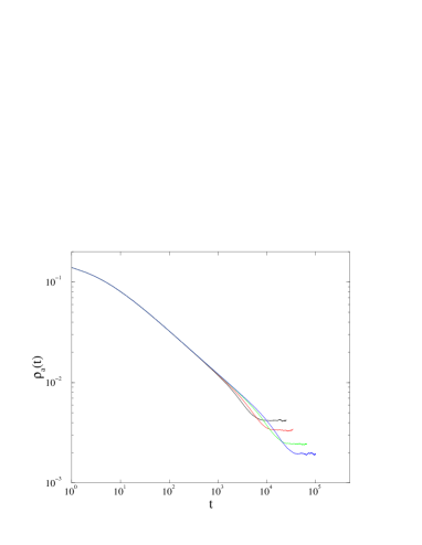
FIG. 1.: Manna FES: active-site density in surviving trials versus time at the critical point, $\zeta=0.71695$. From up to bottom, system sizes $L=192,256,384,512,800$.

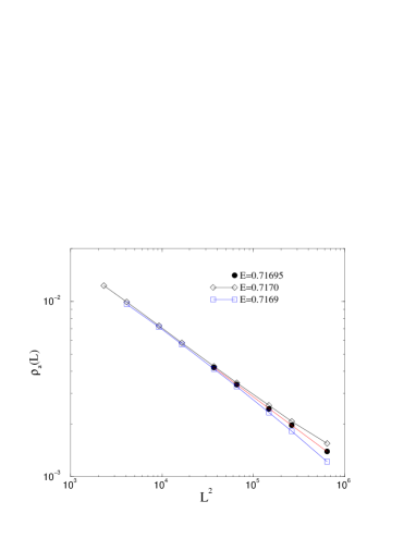
FIG. 2.: Stationary active-site density versus system size in the Manna FES. Sizes range from $L=48$ to $L=800$.

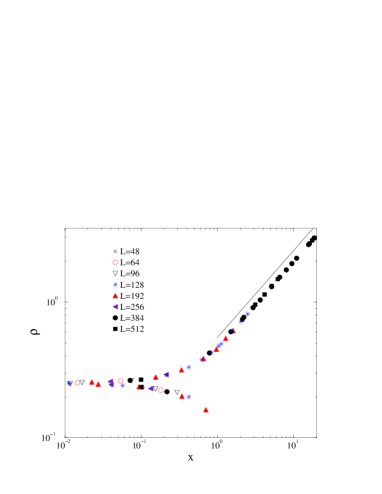
FIG. 3.: Scaling plot of the stationary density $\rho\equiv L^{\beta/\nu_{\perp}}\overline{\rho_{a}}$ versus $x=L^{1/\nu_{\perp}}\Delta$ for various system sizes in the Manna FES. The slope of the straight line is $0.64$.

FIG. 4.: Stationary active-site density as a function of $\Delta=\zeta-\zeta_{c}$ for the Manna FES model with $\zeta_{c}=0.71695$.

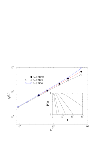
FIG. 5.: Size dependence of $\tau_{P}$ close to the critical point of the Manna FES. The inset shows the power law decay (on a linear-log scale) of the survival probability versus time at $\zeta_{c}=0.71695$ for sizes $L=192,256,384,512,800$ from left to right.

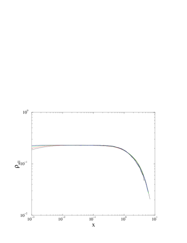
FIG. 6.: Scaling plot of the scaled active-site density $\rho_{all}=\rho_{a,all}(t)t^{\theta}$, in the Manna FES, averaged over all trials versus $x=tL^{-z}$ with $\theta=0.42(1)$ and $z=1.56(3)$. The system size ranges from $L=128$ to $L=800$.

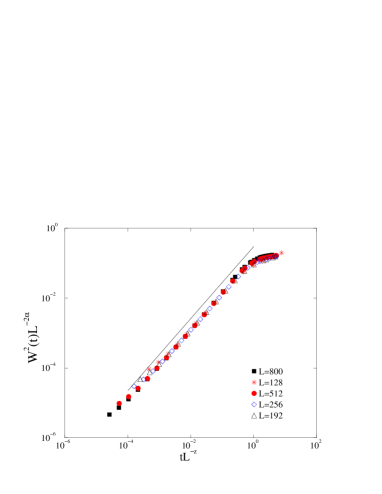
FIG. 7.: Data collapse analysis at $\zeta_{c}=0.71695$ for the interface width $W(t,L)$ of $H(i,T)$, defined as the total number of toppling at time $t$ for each site $i$, in the Manna FES. The exponents used are $\alpha=0.81(2)$ and $z=1.58(3)$.

FIG. 8.: Pair mean-field prediction (line) and simulation results (squares) for the active-site density in the two-dimensional BTW FES.

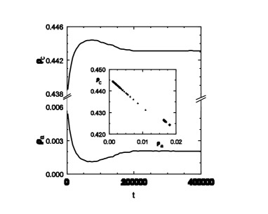
FIG. 9.: Relaxation of the active-site density $\rho_{a}$ (lower graph) and the critical-site density $\rho_{c}$ (upper graph) in the BTW FES at the critical point ($\zeta=2.125$, $L=1280$). Inset: scatter plot of $\rho_{c}$ versus $\rho_{a}$; $\times$: $\zeta=\zeta_{c}$, $L=1280$; $+$: $\zeta=\zeta_{c}$, $L=640$; diamonds: $\zeta=2.13$, $L=320$.

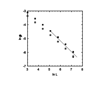
FIG. 10.: Stationary active-site density (open squares) and excess critical-site density (filled squares) versus system size in the BTW FES at $\zeta_{c}$.

FIG. 11.: Relaxation of the active-site density in the BTW FES at $\zeta_{c}$ ($L=320$). Dashed line: unrestricted sample; solid line: sample restricted to runs surviving to $t_{max}=10^{5}$. The inset is a semilog plot of $\rho_{a}(t)$ for the restricted sample.

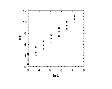
FIG. 12.: Relaxation times versus system size in the BTW FES at $\zeta_{c}$. Open squares: $\tau_{a}$; filled squares: $\tau_{m}$; diamonds: $\tau_{P}$; circles: $\tau_{\overline{P}}$.

FIG. 13.: Initial decay of the active-site density in the BTW FES at $\zeta_{c}$. Solid line: $L=320$; dotted line: $L=640$; dashed line: $L=1280$.

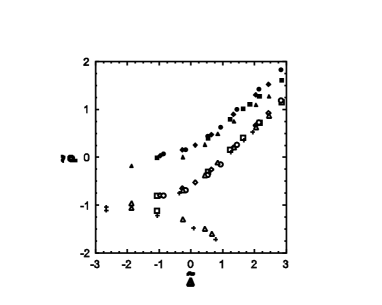
FIG. 14.: Scaled order parameter $\tilde{\rho}$ versus scaled distance from criticality $\tilde{\Delta}$ in the BTW FES. Symbols for the scaled active-site density: $+$: $L=40$; $\triangle$: $L=80$; $\Box$: $L=160$; $\Diamond$: $L=320$; $\circ$: $L=640$. The filled symbols represent the scaled excess critical-site density $\tilde{\rho_{c}}$ for $L=80$, 160, 320, and 640.

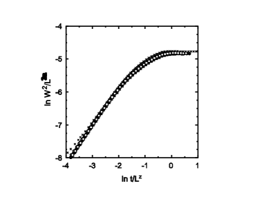
FIG. 15.: Scaling plot of the mean-square interface width $W^{2}(t,L)$ in the BTW FES. $\times$: $L=40$; $\circ$: $L=80$; $\bullet$: $L=160$; $\Box$: $L=320$; filled squares: $L=640$.

FIG. 16.: Main graph: saturation value of the mean-square interface width $W^{2}$ versus system size $L$ in the BTW FES at $\zeta_{c}$. Inset: apparent value of the growth exponent $\beta_{W}$ plotted versus $1/L$.

FIG. 17.: Main graph: histograms for the stationary mean active-site density in a given trial in the BTW FES at $\zeta_{c}$. Dashed line: $L=80$; solid line: $L=160$. The inset shows the evolution of the active-site density in five different trials ($L=80$); the dashed line represents the stationary mean value averaged over a large number of trials.

FIG. 18.: Autocorrelation function for the number of active sites in the BTW FES at $\zeta_{c}$, ($L=80$) averaged over 2000 trials.

FIG. 19.: Autocorrelation function for the number of active sites in the BTW FES at $\zeta_{c}$, ($L=80$) in three different trials.

FIG. 20.: Autocorrelation function for the number of active sites in the BTW FES at $\zeta_{c}$, ($L=80$) in a long trial.

FIG. 21.: Scaling plot of the stationary active-site density $\rho\equiv L^{\beta/\nu_{\perp}}\overline{\rho_{a}}$ versus $x=L^{1/\nu_{\perp}}\Delta$ for various system sizes in the shuffling model. Here $\beta/\nu_{\perp}=0.76$ and $1/\nu_{\perp}=1.266$. The slope of the straight line is $0.60$.

FIG. 22.: Size dependence of $\tau_{P}$ close to the critical point of the shuffling FES. $\diamond$: $\zeta=0.2420$; $\circ$: $\zeta=0.2425$; $\ast$: $\zeta=0.2427$; $\Box$: $\zeta=0.2430$. The inset shows the power-law decay (on a linear-log scale) of the survival probability versus time at $\zeta_{c}=0.20427$ for sizes $L=128,192,256,320$ from left to right.

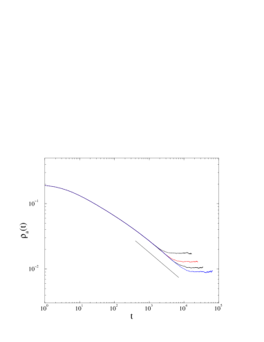
FIG. 23.: Shuffling FES: active-site density in surviving trials versus time at the critical point $\zeta=0.20427$. From up to bottom system sizes $L=128,192,256,320$. The straight line has slope $\theta=0.45$.

REFERENCES

- [1] P. Bak, C. Tang and K. Wiesenfeld, Phys. Rev. Lett. 59, 381 (1987); Phys. Rev. A 38, 364 (1988).
- [2] S. S. Manna, J. Phys. A 24, L363 (1991).
- [3] Y.-C. Zhang, Phys. Rev. Lett. 63, 470 (1989); L.Pietronero, P. Tartaglia and Y.-C. Zhang, Physica A 173, 129 (1991).
- [4] D. Dhar and R. Ramaswamy, Phys. Rev. Lett. 63, 1659 (1989).
- [5] B. Tadic and D. Dhar, Phys. Rev. Lett. 79, 1519 (1997).
- [6] D. Dhar, Phys. Rev. Lett.64, 1613 (1990); S. N. Majumdar and D. Dhar, Physica A 185, 129 (1992); for a review see also D. Dhar, cond-mat/9909009.
- [7] V. B. Priezzhev, J. Stat. Phys. 74, 955 (1994); E. V. Ivashkevich, J. Phys. A 27, 3643 (1994); E. V. Ivashkevich,D.V.Ktitarev and V. B. Priezzhev, Physica A 209, 347 (1994).
- [8] L. Pietronero, A. Vespignani and S. Zapperi, Phys. Rev. Lett. 72, 1690 (1994).
- [9] J. Hasty and K. Wiesenfeld, J. Stat. Phys. 86, 1179 (1997).
- [10] A. Díaz-Guilera, Europhys. Lett. 26, 177 (1994).
- [11] V. B. Priezzhev, cond-mat/9904054.
- [12] T. Hwa and M. Kardar, Phys. Rev. A 45, 7002 (1992).
- [13] G. Grinstein, in Scale Invariance, Interfaces and Nonequilibrium Dynamics, NATO Advanced Study Institute, Series B: Physics, vol. 344, A. McKane et al., Eds. (Plenum, New York, 1995).
- [14] D. Sornette, A. Johansen, and I. Dornic, J. Phys. I (France)5, 325 (1995).
- [15] A. Vespignani and S. Zapperi, Phys. Rev. Lett. 78, 4793 (1997); Phys. Rev. E 57, 6345 (1998).
- [16] R. Dickman, A. Vespignani and S. Zapperi, Phys. Rev. E 57, 5095 (1998).
- [17] A. Vespignani, R. Dickman, M. A. Muñoz, and Stefano Zapperi, Phys. Rev. Lett. 81, 5676 (1998).
- [18] O. Narayan and A. A. Middleton, Phys. Rev. B 49 244 (1994).
- [19] M. Paczuski and S. Boettcher, Phys. Rev. Lett. 77, 111 (1996)
- [20] K. B. Lauritsen and M. Alava, cond-mat/9903346.
- [21] M. Alava and K. B. Lauritsen, cond-mat/0002406.
- [22] Deviations from criticality with respect to the driving field can be obtained in the case of fast driving. See ref.[12] and A. Barrat, A. Vespignani and S. Zapperi, Phys. Rev. Lett. 83, 1962 (1999).
- [23] S. Zapperi, K. B. Lauritsen, and H. E. Stanley, Phys. Rev. Lett. 75, 4071 (1995).
- [24] A. Chessa, E. Marinari and A. Vespignani, Phys. Rev. Lett. 80, 4217 (1998).
- [25] The question of open versus closed models for SOC is also discussed in A. Montakhab and J. M. Carlson, Phys. Rev. E 58, 5608 (1998).
- [26] An early study of sandpiles varying the total energy can be found in C. Tang and P. Bak, Phys. Rev. Lett. 60, 2347 (1988).
- [27] R. Dickman, in Nonequilibrium Statistical Mechanics in One Dimension V. Privman, Ed. (Cambridge University Press, Cambridge 1996); G. Grinstein and M. A. Muñoz, in Fourth Granada Lectures in Computational Physics, Ed. P. Garrido and J. Marro, Lecture Notes in Physics, 493, 223 (Springer-Verlag, Berlin, 1997). J. Marro and R. Dickman, Nonequilibrium Phase Transitions in Lattice Models (Cambridge University Press, Cambridge, 1999).
- [28] See H. Leschhorn, T. Nattermann, S. Stepanow and L-H. Tang, Ann. Phys. 6, 1 (1997), and references therein.
- [29] O. Narayan and D. S. Fisher, Phys. Rev. B 48 7030 (1993).
- [30] Like any other statistical model, a fixed-energy sandpile exhibits critical singularities only in the infinite-size limit. In this limit the activity density is strictly zero for , and positive for , ensuring the stated inequality for in the slowly-driven system.
- [31] D.Dhar, Physica A 270, 69 (1999).
- [32] S. Maslov and Y-C. Zhang, Physica A 223, 1 (1996).
- [33] J.L. Cardy and R.L. Sugar, J. Phys. A 13, L423 (1980); P. Grassberger, Z. Phys. B 47, 365 (1982); H.K. Janssen, Z. Phys. B 42, 151 (1981).
- [34] The connection with the RFT theory has been also discussed for the Bak-Sneppen SOC model. S.Maslov, M. Paczuski and P. Bak, Europhys. Lett. 27, 97 (1994); P. Grassberger, Phys. Lett. A 200, 277 (1995).
- [35] P. Grassberger and S. S. Manna, J. Phys. (France) 51, 1077 (1990).
- [36] S. S. Manna, J. Stat. Phys. 59, 509 (1990).
- [37] S. Lübeck and K.D. Usadel, Phys. Rev. E 55, 4095 (1997); ibid. 56, 5138 (1997).
- [38] M. De Menech, A. L. Stella and C. Tebaldi, Phys. Rev. E 58, R2677 (1998); C. Tebaldi M. De Menech and A. L. Stella, Phys. Rev. Lett. 83, 3952 (1999).
- [39] This is the inclusive version of the Manna model. Is it also possible to define an exclusive version in which the two toppling particles are forbidden to go to the same neighbor site: H. Kobayashi and M. Katori, J. Phys. Soc. Jpn. 66, 2367 (1997).
- [40] A. Ben-Hur and O. Biham, Phys. Rev. E 53, R1317 (1996).
- [41] A. Chessa, H. E. Stanley, A. Vespignani and S. Zapperi, Phys. Rev. E 59, R12 (1999).
- [42] S. Lübeck,Phys. Rev. E 61, 204 (2000).
- [43] A. Chessa, A. Vespignani and S. Zapperi, Comput. Phys. Comm. 121-122, 299 (1999).
- [44] R. Pastor-Satorras, private communication.
- [45] P. Grassberger, private communication.
- [46] In the BTW model, one actually encounters immortal configurations — in which activity never ceases — having . The probability of generating such an initial configurations decays rapidly with system size, and in practice we have not seen them for .
- [47] W. Kinzel, Z. Phys. B58, 229 (1985).
- [48] T. M. Ligget, Interacting Particle Systems, (Springer Verlag, New York, 1985).
- [49] While our ansatz simplifies the analysis of stationary states, a theory of transient or spreading dynamics may require retaining as an independent field, if its initial value differs from the stationary one, . The situation is analogous to that of a ‘non-natural’ initial density in the PCP [82].)
- [50] A. J. Bray, Adv. in Phys., 43, 357 (1994).
- [51] This is the case of branching, annihilating random walks with even numbers of offspring, also known as the “parity conserving” or “directed Ising” universality class. See: P. Grassberger, F. Krause, and T. von der Twer, J. Phys. A 17, L105 (1984); P. Grassberger, ibid. 22, L1103 (1989); H. Takayasu and A. Yu. Tretyakov, Phys. Rev. Lett. 68, 3060 (1992); I. Jensen, Phys. Rev. E 50, 3623 (1994); N. Menyhard and G. Ódor, J. Phys. A 29, 7739 (1996); J. Cardy and U. C. Täuber, Phys. Rev. Lett. 77, 4780 (1996). H. Hinrichsen, Phys. Rev. E 55, 219 (1997); W. Hwang, S. Kwon, H. Park, and H. Park, Phys. Rev. E 57, 6438 (1998).
- [52] M. A. Muñoz, R. Dickman, A. Vespignani and S.Zapperi, preprint (1999).
- [53] A.J. Noest, Phys. Rev. Lett. 57, 90 (1986).
- [54] A.G. Moreira and R. Dickman, Phys. Rev. E 54, R3090 (1996).
- [55] A.J. Noest, Phys. Rev. B 38, 2715 (1988).
- [56] R. Dickman and A.G. Moreira, Phys. Rev. E 57, 1263 (1998).
- [57] R. Calfiero, A. Gabrielli, and M. A. Muñoz, Phys. Rev. E 57, 5060 (1998).
- [58] In the former case, e.g., for a site-diluted contact process [54], activity tends to be restricted to favorable regions (lower than average dilution). In the present case, it is principally at the boundaries between active and inactive regions that, as implied by the Laplacian in Eq. (1), energy is transferred, and the effect is to move energy into the inactive region, thereby enhancing the further spread of activity. Indeed, the simulations reported below reveal none of the hallmarks of quenched disorder in the contact process, such as logarithmic time-dependence in critical spreading, or generic power-law relaxation of temporal correlations [54, 55, 56, 57].
- [59] H. K. Janssen, Phys. Rev. E 55, 6253 (1997).
- [60] Remarkably, the opposite identification is also possible in certain cases. See U. Alon, M. R. Evans, H. Hinrichsen, and D. Mukamel, Phys. Rev. Lett. 76, 2746 (1996).
- [61] Note that in the case of quenched point disorder the “automaton” dynamics (i.e., when the local velocity can only take the values ) is found to be in the same universality class as the continuous equation [28].
- [62] A. -L. Barabási and H. E. Stanley, Fractal Concepts in Surface Growth, (Cambridge University Press, Cambridge, 1995).
- [63] G. Parisi and L. Pietronero, Europhys. Lett. 16, 321 (1991); Physica A 179, 16 (1991).
- [64] It has been pointed out that the -function leads to an additional effective noise term [20], which could imply a different universality class for the automaton model and the continuous equation.
- [65] Note that the quenched disorder present in the LIM equations is mimicked in the RFT representation by the site-dependent non-Markovian term. The general equivalence between quenched noise and non-Markovian evolution has been pointed out in the context of the so-called run-time-statistics; see M.Marsili, J. Stat. Phys. 77, 733 (1994).
- [66] F. Family and T. Vicsek, J. Phys. A 18, L75 (1985).
- [67] J. M. López, Cond-mat/9910167. To appear in Phys. Rev. Lett. See also J. Kertesz and D. E. Wolf, Phys. Rev. Lett. 22, 2571 (1989); S. Das Sarma et al. Phys. Rev. E 53, 359 (1996); J. M. López and M. A. Rodríguez, Phys. Rev. E 56, 3993 (1997); J. Phys. I 7, 1191 (1997).
- [68] N-N. Pang and W-J. Tzeng, Phys. Rev. E 59, 234 (1999).
- [69] R. Pastor-Satorras and A. Vespignani, cond-mat/9907307.
- [70] M. E. Fisher, in Proceedings of the International Summer School ‘Enrico Fermi’, Course LI, (Academic Press, New York, 1971); M. E. Fisher and M. N. Barber, Phys. Rev. Lett. 28, 1516 (1972).
- [71] R. Dickman, M. Alava, M. A. Muñoz, J. Peltola, A. Vespignani, and S. Zapperi, in preparation.
- [72] It is likely that, in fact, is the exact result, as can be verified by using Priezzhev’s results [7]. Grassberger, private communication.
- [73] The strict linear relationship between and supports our elimination of as an independent field, in the continuum description developed in Sec. III.
- [74] H. K. Janssen, B. Schaub and B. Schmittmann, Z. Phys. B 73, 539 (1989).
- [75] That is insensitive to a change in the order of updating lends some support to the assertion that average properties are not strongly dependent on the kind of updating used for the BTW model.
- [76] D. V. Ktitarev, S. Lubeck, P. Grassberger, and V. B. Priezzhev, cond-mat/9907157.
- [77] M. A. Muñoz, R. Dickman, A. Vespignani, and Stefano Zapperi, Phys. Rev. E 59, 6175 (1999).
- [78] R. Dickman, cond-mat/9909347.
- [79] I. Jensen, Phys. Rev. Lett. 70, 1465 (1993); I. Jensen and R. Dickman, Phys. Rev. E 48, 1710 (1993).
- [80] J.F.F Mendes, R. Dickman, M. Henkel, and M.C. Marques, J. Phys. A 27, 3019 (1994).
- [81] M. A. Muñoz, G. Grinstein, R. Dickman and R. Livi, Phys. Rev. Lett. 76, 451, (1996).
- [82] M. A. Muñoz, G. Grinstein, and R. Dickman, J. Stat. Phys. 91, 541-569 (1998).
- [83] S.-D. Zhang, Phys. Rev. E 60, 259 (1999).
- [84] M. Doi, J. Phys. A9, 1465 (1976). L. Peliti, J. Physique 46, 1469 (1985). B. P. Lee and J. Cardy, J. Stat. Phys. A 80, 971 (1995).