Glass transition of a particle in a random potential, front selection in non linear RG and entropic phenomena in Liouville and SinhGordon models

Abstract

We study via RG, numerics, exact bounds and qualitative arguments the equilibrium Gibbs measure of a particle in a $d$-dimensional gaussian random potential with translationally invariant logarithmic spatial correlations. We show that for any $d\geq 1$ it exhibits a transition at $T=T_{c}>0$. The low temperature glass phase has a non trivial structure, being dominated by a few distant states (with replica symmetry breaking phenomenology). In finite dimension this transition exists only in this “marginal glass” case (energy fluctuation exponent $\theta=0$) and disappears if correlations grow faster (single ground state dominance $\theta>0$) or slower (high temperature phase). The associated extremal statistics problem for correlated energy landscapes exhibits universal features which we describe using a non linear (KPP) RG equation. These include the tails of the distribution of the minimal energy (or free energy) and the finite size corrections which are universal. The glass transition is closely related to Derrida’s random energy models. In $d=2$, the connexion between this problem and Liouville and sinh-Gordon models is discussed. The glass transition of the particle exhibits interesting similarities with the weak to strong coupling transition in Liouville ($c=1$ barrier) and with a transition that we conjecture for the sinh-Gordon model, with correspondence in some exact results and RG analysis. Glassy freezing of the particle is associated with the generation under RG of new local operators and of non-smooth configurations in Liouville. Applications to Dirac fermions in random magnetic fields at criticality reveals a peculiar “quasi-localized” regime (corresponding to the glass phase for the particle) where eigenfunctions are concentrated over a finite number of distant regions, and allows to recover the multifractal spectrum in the delocalized regime.

I introduction

Despite significant progress in the last two decades, disordered systems continue to pose considerable theoretical challenges. Two important questions still largely open, are, respectively, to which extent the (better understood) mean field models are relevant to describe low dimensional physical systems, and, in the special case of two dimension, to which extent the powerful field theoretic treatments developed for pure models can be adapted to treat disordered models.

A celebrated controversy is whether the structure found in the solution of mean field models for spin glasses and other complex disordered systems, both in the statics [2] and in the dynamics [3], has any counterpart in the world of experimentally relevant low dimensional models. Specifically it has been vigorously questionned [4] whether the breaking of the phase space in “many pure states”, predicted to occur in mean field, may also occur in short range models, and how it can be properly defined [5, 6]. The unusual nature of the technique used to solve the statics, i.e the replica method with a hierarchical breaking of the permutation symmetry between replicas in the limit $n\to 0$ (RSB), did not contribute to make the physics transparent. A distinct structure, which remarkably parallels the one in the statics, has been found [3] to occur in the nonequilibrium dynamics. The dynamical problem can be studied by a priori better defined methods and leads to predictions which are in principle directly testable in experiments, such as a non trivial generalization of the fluctuation dissipation relations. Even so, it has been emphasized that mean field models, which usually involve infinite range or infinite number of component limits, may not capture physical processes important in low dimensions. The alternative “droplet picture” in its simplest form [4] postulates the existence of a single ground state with excitations (droplets) of (free) energy $\Delta E$ scaling with their size $x$ as $\Delta E\sim x^{\theta}$, $\theta>0$. It provides a more conventional scaling description of the glass physics, as being controlled by zero temperature RG fixed points where temperature is formally irrelevant (with eigenvalue $-\theta$).

Another important advance was the exact solution of simpler prototype models, such as the random energy model (REM) [7], where one consider simply a collection of independently distributed energy levels, as well as its generalization, the GREM [8], or the Directed Polymer on the Cayley Tree (DPCT) with disorder [9]. These solutions being direct with no use of replica, their results can be fully relied upon. They exhibit a similar physics though, with a glass transition and in the glass phase, an exponential tail for the distribution of the free energy $P(f)\sim e^{\beta_{c}f}$ for negative $f$. This feature is crucial to recover the same physics, and indeed many observables were found to be similar [10]. In fact the alternative solution of the REM using replicas, given in [7] or the one of the DPCT [11] do involve RSB. In the REM model the structure of the glass phase is particularly transparent as being dominated by a few states [7, 10].

It is important to go beyond models defined in mean field or on hierarchical (or ultrametric) structures and to study simple yet non trivial (and non artificial) finite $d$ models with full statistical translational invariance. In this paper we study the model of a particle in a gaussian random potential $V(\bf{r})$ with spatial correlations which are invariant by translation and which grow as the logarithm of the distance. We consider this model in any dimension $d$, but in $d=2$ it has also been studied recently since it is of direct relevance for several physical systems [12, 13, 14, 15, 16, 17, 18, 19, 20]. One example is a spin model with $XY$ symmetry and random gauge quenched disorder, which arises naturally in describing Josephson junction arrays [21] or 2D crystalline structures with smooth disorder, e.g. flux lattices in superconductors [22], or electrons at the surface of Helium [23]. In this model, a single topological defect (a $XY$ vortex), or a single neutral pair, sees precisely a random potential with logarithmic correlations [15, 16, 17, 18, 19]. Another example arises in a model of localization of Dirac fermions in a random magnetic field, motivated by quantum Hall physics. There, the zero energy $E=0$ normalized wavefunction is identical to the Boltzmann weight of the particle studied here [12, 13, 14]. This wave function is “critical” in a sense discussed below.

Here we study this model using a renormalization group (RG) approach, bounds, numerical methods and qualitative arguments. We show that it exhibits a transition at $T=T_{c}>0$ in any $d\geq 1$. We find that in the high temperature phase the particle is essentially delocalized over the whole system, while in the low temperature glass phase the Gibbs measure is concentrated in a few minima. The fact that such a simple (finite $d$) model exhibits a genuine glass transition is already surprising. Indeed, as we argue, this transition exists only for such a “marginal” type of correlations (which correspond to $\theta=0$ in the glass scaling mentionned above [24]). It disappears (for gaussian $V({\bf{r}})$) if correlations grow faster (with only a low temperature phase and single ground state dominance) or slower (with only a high temperature phase). Logarithmic growth of correlations thus produces exactly the right balance between the depth of the energy wells and their number (entropy). Note that for slower growing correlations one can recover a transition but only by artificially rescaling the disorder variance with the size of the system: in the extreme case of uncorrelated variables, it is the REM model. Here by contrast, there is a genuine phase transition in the thermodynamic limit, with no need for rescaling. Most interestingly, the glass phase is non trivial. The Gibbs measure is concentrated in a few distant minima which remain in a finite number in the thermodynamic limit. This is because the extrema of random variables with such correlations exhibit an interesting property of “return near the minimum”: there is, with a finite probability in a sample of size $L\to+\infty$, at least one second minimum far away (at distances of order $L$), and with a finite energy difference with the absolute minimum. And there are not too many (a thermodynamic number) of these secondary minima, leading to a zero entropy. As in the REM, this property leads here naturally to a non trivial ground state structure, reminiscent as we discuss of a genuine property of replica symmetry breaking in the replicated theory. The low temperature limit corresponds to a non trivial problem of extremal statistics of correlated variables, studied here.

Another interesting property of this model is its relation to the Liouville model (LM) and the sinhGordon model (SGM) in $d=2$ (and their boundary restriction in $d=1$): $V({\bf r})$ turns out to be the Liouville field while the LM and SGM partition functions arise simply as generating functions of the probability distribution of the partition sum $Z[V]=\int_{\bf r}e^{-\beta V({\bf r})}$ of a single particle. The high temperature phase for the particle corresponds to the weak coupling regime for the LM and SGM, where we find that known exact results compare well with results for the particle. In the SGM we predict here the existence of a transition (more appropriately, a “change of behaviour”). It corresponds to the glass transition for the particule, which also exhibits interesting similarities with the weak to strong coupling transition in the Liouville theory (and the so called $c=1$ barrier). The glassy freezing of the particule is associated, in the LM and SGM, to new local operators and non smooth configurations being generated under RG.

To study the model we will introduce a RG approach based on a Coulomb gas renormalization a la Kosterlitz. It leads to a non linear RG equation (of the so-called Kolmogorov KPP type) for the full probability distribution of the “local disorder”. Indeed, a separation between the long range part of the disorder and the local, short range part, arises naturally in our approach. The RG equation has traveling wave types of solutions. The corresponding well known problem, in such non linear equations, of the selection of the velocity of the traveling front, and its freezing for $T\leq T_{c}$ is related to glassy freezing of the particle free energy and, in the LM or SGM, to the “selection” of the anomalous dimensions (and at the transition dimension degeneracy leads to logarithmic operators). When temperature is lowered the local disorder becomes broadly distributed and the freezing occurs when its tails become relevant. Our RG method indicates that the physics depends only weakly of $d$. We will take advantage of this fact and check our results using simulations in $d=1$.

It is important to compare the present work to previous studies of the model. The existence of a freezing transition in $d=2$ has been conjectured previously [18, 16, 17] based on an approximation which completely neglect spatial correlations (REM approximation, see below). Stronger arguments were given in [14], but did not fully establish the existence of a transition, which is done here (see Appendix (A)). The present work is thus motivated by the need to go beyond the REM approximation to describe this problem. In particular one wants to know what is the precise universality class of the model, which we hope can be determined from the RG method introduced here. This RG method yields some remarkable universal features of the probability distribution of the free energy and of its finite size corrections, different from the REM. It shows that the problem is more closely related to the directed polymer on a Cayley tree. A qualitative analogy between the present model and the DPCT was in fact cleverly guessed recently in Ref. [17, 12]. It is based on the observation that the energy of polymer configuration on a tree also scale logarithmically with the overlap distance defined on the tree (see Fig 1). It is remarkable that this connection naturally emerges here from the Kosterlitz type RG performed on this problem, via the KPP equation. It is all the more surprising, since the model studied here has statistical translational invariance, while a tree has a hierarchical structure. The solution of Derrida and Spohn [9] (and the mapping onto the DPCT proposed in [17, 12]) would be exact for random variables $V({\bf r})$ correlated with a hierarchical (i.e ultrametric) matrix of correlation. Here instead the correlations are translationally invariant and it is thus important to understand the origin of the analogy with the DPCT and to which extent it holds. The RG procedure developed in this paper is a first attempt to address these questions. The result is that we can make the mapping precise: at least for the universal observables studied here (e.g. the tails of the free energy distribution), the mapping is onto a continuum branching process, i.e a continuum limit of a Cayley tree (whereas [17, 12] could not be so specific).

FIG. 1.: Directed polymer approximation: sites are the tree endpoints. The $v^{p}_{q}$ are uncorrelated of variance $2\sigma$. The random potential at $i$ is $V_{i}=v^{(1)}_{1}+v^{(2)}_{1}+v^{(3)}_{2}$ and at $j$ it is $V_{j}=v^{(1)}_{1}+v^{(2)}_{2}+v^{(3)}_{4}$. Thus $\overline{(V_{i}-V_{j})^{2}}=4\sigma d(i,j)$ where $d(i,j)\sim\ln|i-j|$ is the distance (in generations) on the tree

The present model has also been studied in the context of random Dirac problems and localization. An early study [25] of the $E=0$ wavefunction established that it was critical (in the sense of corresponding to a “delocalized” wave function, while $E\neq 0$ has finite localization length). However this study missed the glass transition. Later studies [14] computed the multifractal spectrum based on the REM approximation and noticed the existence of a strong disorder regime. These and other studies [12, 13] however focused on properties of the high temperature phase: it was conjectured [13] that the (conformal) Liouville field theory (LFT) (i.e a continuum limit of the LM) was able to describe all spatial correlations of the model in the high temperature phase. These works call for more investigations. First the glass transition and the peculiar physical properties of the low T (i.e strong disorder) phase have not been addressed, even at the most qualitative level. We thus find it useful to present the problem from a different perspective by comparing with other types of correlated disorder, or by recasting it as a problem of extremal statistics. Although well known properties [26] of extremal statistics of uncorrelated variables were often used to study model disordered systems (see e.g. [27, 28, 29]) a lot remains to be understood about the (more realistic) case of correlated variables. Second, the question of the universality class is in our opinion far from established. Evidence for the LFT description mostly comes from reproducing the multifractal spectrum as given by the REM approximation and one would like to check it against more detailed predictions. The present RG procedure is a step towards clarifying the connexion between this model and solvable models such as Derrida’s REM and Derrida-Spohn DPCT. In this respect finite size corrections are important to understand, as they are found to exhibit universal prefactors allowing to distinguish between various universality classes. In addition, they determine the anomalous dimensions, and thus control the critical behaviour, in the full disordered XY model as shown in [19]. Since they are found to be very large, they are also crucial in order to analyze the results of numerical simulations. In particular, although we confirm the result of [12], we also conclude that the sizes used in the numerical study of [12] were in fact vastly insufficient for drawing firm conclusions: we do perform here a more detailed finite size analysis on much larger samples to confirm analytical predictions.

The model studied here is thus related to a surprising number of interesting problems. Let us mention for completeness that it also has connexions to problems such as two dimensional interfaces, or films, confined between two walls (for $\beta=+\infty$ it is the confinement entropy of a film), wetting transitions [30], extremal statistics of correlated variables useful e.g. for problems of “persistence” in nonequilibrium dynamics [31], and finally, to the clumping transition of a self gravitating planar gas [32]. We will not explore these connections in details here.

This paper is organized as follows: in section II, the single particle model is defined and in section II B the random energies approximation (REM) is applied, which amounts to neglect the spatial correlations of the random potential. The full problem, with correlations taken into account, is related to the description of extremal statistics in II C, and three different classes of correlations are identified in II D from qualitative arguments. A new renormalization (RG) technique is applied to this problem in section III. The resulting non-linear scaling equation for the distribution of the local disorder is studied in section III C, and found to be related to the Kolmogorov KPP equation, which admits front solutions. This connection between front solutions of non-linear equations and the renormalization of disordered models is pursued in section III D, where a solution to the REM is found via a similar non-linear RG (details in Appendix C). The non trivial nature of the glass phase is discussed in III E together with its relations to replica symetry breaking. In part IV we present a numerical analysis of the problem of the particle in a random potential in $d=1$. Section V is devoted to the connexion between the particle model -and its transition- and entropic phenomena in the Liouville and Sinh-Gordon models. A direct RG analysis in Section V C allows to recover the corresponding change of behaviours in these models. Section VI contains the applications to the properties of the critical wave function of a Dirac fermion in a random magnetic field, in particular the multifractal properties and the property of quasi-localization. Appendix A contains an outline of the proof of the existence of a transition, Appendix B is a review of well known (and not so well known) results about extremal statistics, Appendix D contains an extended model which exhibits three phases.

II Model and qualitative analysis

In this Section we define the model of a single particle in a correlated random potential. Then we describe the random energy model (REM) approximation used in previous studies which consist in neglecting correlations. We then pose the new questions which we want to address here for the true model and present a qualitative analysis showing physically why we expect that logarithmic correlations (as opposed to faster growing or slower growing correlations) is the only case which leads to (i) a glass transition (ii) a low temperature phase with a non trivial structure of quasi degenerate distant minima

A the model

The equilibrium problem of a single particle in a $d$-dimensional random potential is defined by the canonical partition function

$$Z[V]=\sum_{{\bf r}}e^{-\beta V({\bf r})}$$ (1)

where $\beta=1/T$ is the inverse temperature, in a sample of finite size $L$ (and total number of sites $L^{d}$) and for a given configuration of the random variables $V({\bf r})$. The equilibrium Gibbs measure, or probability distribution for the position of the particle is:

$$p({\bf r})=e^{-\beta V({\bf r})}/Z[V]$$ (2)

We are interested here in cases where the random variables $V({\bf r})$ can be correlated. As discussed below, the statics (and dynamics) of this problem in the limit of large sizes depends on the type of correlations, the distribution of the disorder and the dimensionality of space $d$. Some of these cases and their dynamical aspects (such as the Sinai model) have been extensively studied, e.g. in the context of diffusion in random media [33]. Even logarithmic correlations in $d=2$ were studied then [34], but it was not realized at that time that a static glass transition could exist in that case.

Correlated random potentials $V({\bf r})$ are most conveniently studied for Gaussian distributions, on which we focus, parametrized by the correlator $\Gamma({\bf r},{\bf r}^{\prime})=\overline{V({\bf r})V({\bf r}^{\prime})}$ (and we choose $\overline{V({\bf r})}=0$). Non gaussian extensions will be mentionned. Unless specified otherwise the correlations will be chosen translationally invariant $\Gamma({\bf r},{\bf r}^{\prime})=\Gamma_{L}({\bf r}-{\bf r}^{\prime})$ with cyclic boundary conditions, or in (discrete) Fourier space $\overline{V({\bf q})V({\bf p})}=\Gamma({\bf q},{\bf p})=\Gamma({\bf q})\delta_{{\bf p},-{\bf q}}$. We will often denote $\overline{(V({\bf r})-V({\bf r}^{\prime}))^{2}}=\tilde{\Gamma}({\bf r}-{\bf r}^{\prime})=2\int_{\bf q}\Gamma({\bf q})(1-\cos({\bf q}.({\bf r}-{\bf r}^{\prime})))$ (with $\int_{\bf q}=\frac{1}{L}\sum_{\bf q}\to\int\frac{d^{d}{\bf q}}{(2\pi)^{d}}$).

One important quantity is the free energy:

$$F[V]=-T\ln Z[V]$$ (3)

and, since it fluctuates from configuration to configuration, as $F[V]=\overline{F[V]}+\delta F[V]$ we will be interested in its average $F=\overline{F[V]}$ and in its distribution. From the convexity of the logarithm follows the well known exact bound for $F$ in terms of the annealed free energy $F_{A}$:

$$-T\overline{\ln Z}=F\geq F_{A}=-T\ln\overline{Z}$$ (4)

$$F\geq-(Td\ln L+\frac{1}{2T}\overline{V(\bf{r})^{2}})$$ (5)

for the Gaussian case.

In this paper we will mainly focus on the case of correlations growing logarithmically with distance:

$$\overline{(V({\bf r})-V({\bf r}^{\prime}))^{2}}\sim 4\sigma\ln\frac{|{\bf r}-{\bf r}^{\prime}|}{a}\qquad a\ll|{\bf r}-{\bf r}^{\prime}|\ll L$$ (6)

which also requires a small distance ultraviolet (UV) cutoff $a$ (we can set here $a=1$ in accordance with the definition 1 of a discrete model, but in the following Sections we will consider a continuum version and vary $a$). This behaviour is achieved in $d$ dimension by choosing a propagator in Fourier space $\Gamma({\bf q})\sim\frac{2\sigma(2\pi)^{d}}{S_{d}q^{d}}$. The $d=2$ case is also of special interest as the propagator is the usual Coulomb one:

$$\Gamma({\bf q})\sim\frac{4\pi\sigma}{q^{2}}$$ (7)

and boundary conditions must be specified later on. It is important to note that for LR correlations the single site variance $\overline{V({\bf r})^{2}}=\Gamma_{L}(0)$ diverges with the system size, e.g. for (6) one has $\Gamma_{L}(0)\sim 2\sigma\ln(L/a)$.

For such logarithmic correlations (as well as for weaker correlations [35]) one will find that $F$ scales as $d\ln L$ (consistent with the number of degree of freedom being $L^{d}$ in this problem). Thus it is natural to define the intensive free energy:

$$f(\beta)=\lim_{L\to+\infty}\frac{F[V]}{d\ln L}$$ (8)

which will be found to be self averaging. The above bound gives:

$$f(\beta)\geq-\left(\frac{1}{\beta}+\frac{\sigma}{d}\beta\right)$$ (9)

Thus we will find that $F[V]\sim f(\beta)d\ln L$ with subdominant corrections. These corrections have a non fluctuating universal $O(\ln(\ln L))$ piece, as well as an $O(1)$ fluctuating part $\delta F[V]$ which we will both study.

B the REM approximation

A useful approximation to the problem studied here, which can be called the REM approximation, consists in neglecting all correlations but keeping the on site variance exact [18, 14]:

$$\Gamma_{L}({\bf r})\to\Gamma^{{\rm REM}}_{L}({\bf r})=\Gamma_{L}(0)\delta_{{\bf r},{\bf r}^{\prime}}=2\sigma\ln\left(\frac{L}{a}\right)\delta_{{\bf r},{\bf r}^{\prime}}$$ (10)

The corresponding Gaussian REM model can then be solved, being identical to [7], and one finds that it exhibits a transition at $\beta_{c}=\sqrt{d/\sigma}$ with:

$$f(\beta)=-\left(\frac{1}{\beta}+\frac{\sigma}{d}\beta\right)\qquad\beta<\beta_{c}$$ (11a)

$$f(\beta)=-\frac{2}{\beta_{c}}\qquad\beta>\beta_{c}$$ (11b)

Most previous studies of the original model (all in $d=2$) amount to study the REM approximation and argue that it is a good approximation. Indeed, as we will also find here, this REM approximation appears to give the exact result for some observables (e.g. for $f(\beta)$). In particular, it does seem to give correctly the transition temperature $\beta_{c}$.

C beyond the REM approximation: extremal statistics of correlated variables

Since it is not obvious a priori why logarithmic correlations can be considered so weak as to be neglected, one would like to go beyond the REM approximation and describe the effect of the neglected correlations [36]. One would like to understand why this approximation works for some observables (and for which ones) and whether it gives exactly the universality class of the model (i.e all universal behaviour of observables). The answer to the latter is negative: as our analysis will reveal, the correlations do matter for the more detailed behaviour and the original model (1,6) is not in the same universality class as the REM model.

In fact, the problem at hand is related to describing universal features of the extremal value statistics for a set of correlated random variables. Indeed, the zero temperature limit ($T=0$ for fixed $L$) of the problem defined by (1) amounts to finding the distribution of the minimum $-\lim_{T\to 0}T\ln Z_{L}=V_{min}=min_{r}(\{V_{r}\})$ of a set of correlated random variables. In the case of uncorrelated (or short range correlated) variables a lot is known in probability theory on this problem (see e.g. [37]), some of which is summarized in Appendix B. For the type of distributions considered here (gaussian and some extensions) the distribution of the minimum $V_{min}$ has a strong universality property, being given, up to - non trivial - rescaling and shift (see Appendix B and below), by the Gumbell distribution:

$$\text{Proba}(y<x)={\cal G}(x)=\exp(-e^{x})$$ (12)

The Gumbell distribution thus appears as the distribution of the zero temperature free energy in the REM. For the case of a Gaussian distribution the standard probability theory results are usually given in terms of a variable $X_{r}$ such that $\overline{X_{r}^{2}}=1$. One can simply rescale $V_{r}=\sqrt{2\sigma\ln L}X_{r}$ from Appendix B and get:

$$V_{min}=2\sqrt{\sigma d}\ln L-\frac{1}{2}\sqrt{\frac{\sigma}{d}}\ln(4\pi d\ln L)+\sqrt{\frac{\sigma}{d}}y$$ (13)

where $y$ is distributed as in (12).

Much less is known in the case of variables with stronger correlations studied here, though it is more important in practice. The statistics of $V_{min}$ in the logarithmically correlated case is thus one of the open issues discussed here. One key question is to determine what is universal in the distribution of the minimum of correlated variables. Here, we can formulate the question as follows: given Gaussian random variables satisfying (6), what in the distribution of the minimum (i.e of the ground state energy for fixed large $L$) is universal, i.e depends only on $\sigma$ and not on the details of the correlator $\Gamma({\bf r})$ at short scale. Writing

$$V_{min}\sim\overline{V_{min}}+\delta V_{\min}$$ (14)

one finds, for the logarithmic correlator, that the averaged ground state energy must satisfy:

$$\overline{V_{\min}}\geq-2\sqrt{\sigma d}\ln L$$ (15)

which follows from the above annealed bound, together with the fact that $\partial f/\partial T=-S\leq 0$. Furthermore one will find here that $V_{\min}\sim e_{min}d\ln L$ up to a positive subdominant - universal - piece and that $e_{min}=-2\sqrt{\sigma/d}$ saturates the bound. In the distribution of $\delta V_{\min}\sim O(1)$ we can clearly expect less universality that in the problem of random variables with short range correlations [38].

D Qualitative study of a particle in a random potential

Before describing the RG method which allows to go beyond the REM approximation, let us give some simple qualitative arguments and numerical results which illustrate the main physics of the thermodynamics of a particle in a correlated random potential. To put things in context we discuss several types of correlations (short range, long range, and marginal). We focus on $d=1$ for simplicity but the arguments extend to any finite $d$.

Whether there is a single phase or not here comes simply from whether the entropy of typical sites wins or not over the energy of the low energy sites. When there is a low temperature phase, to decide its structure one must pay special attention to distant secondary local minima.

Indeed, when there is a low temperature phase, it is controlled by the regions with most negative potential. To investigate its structure one can start, for a given system of size $L$, with the $T=0$ state which is determined by the absolute minimum over the system, denoted $V_{min}$ and located at ${\bf r}_{min}$. At $T$ very small but strictly positive, each (low lying) secondary local minima $V$ will also be occupied with a probability $\sim e^{-(V-V_{\min})/T}$ which is very small except when $V-V_{min}\sim O(T)$. Thus to characterize the low temperature phase we need to know how many of these secondary minima exist and where they are located. For a smooth enough disorder (see e.g. Fig 3) there will always be “trivial” secondary local minima in the vicinity of $r_{min}$. To eliminate these, we define $V_{min2}(R)$ as the next lowest minimum constrained to be at a distance at least $R$ of the absolute minimum. An interesting quantity to study is then the distribution $P_{R,L}(\Delta E)$ of $\Delta E(R,L)=V_{min2}(R)-V_{min}$ over environments (which a priori depends on $R$ and $L$)

FIG. 2.: Three cases for the distribution of energy difference $\Delta E$ between absolute and secondary minimum (separated at least by $R\sim L^{c}$) in a system of size $L$: (a) short range correlated potentials, $\Delta E_{typ}\to 0$ logarithmically with size (b) algebraically growing correlations $\Delta E_{typ}\to+\infty$ (c) logarithmic correlations, $\Delta E_{typ}$ remains constant as the system size increases.

We now distinguish three main cases, according to the behaviour of the correlator $\overline{(V({\bf r})-V({\bf r}^{\prime}))^{2}}=\tilde{\Gamma}({\bf r}-{\bf r}^{\prime})$ at large scale (we restrict to gaussian potentials [39]). In these three cases the distribution $P_{R,L}(\Delta E)$ has markedly different behaviours as illustrated in Fig. 2:

(i) short range correlations. i.e $\tilde{\Gamma}({\bf r})\to Cst$ at large ${\bf r}$, equivalently $\Gamma_{L}({\bf r})\to 0$ at large ${\bf r}$ (or e.g. $\Gamma_{{\bf q}}\sim q^{-d+\delta}$ with $\delta>0$). In this case it is clear that there is only a high temperature phase in any finite $d$ and no phase transition. The entropy $Td\ln L$ of typical sites (of energy typically $\sim O(1)$) always wins over the energy of optimal sites ($V_{\min}\sim\sqrt{2\sigma d\ln L}$ for gaussian distributions with on-site variance $\sigma$ ). The optimal energy $V_{min}$ can be estimated using $1/L^{d}=\int_{-\infty}^{V_{min}}P_{1}(V)dV$ in terms of the single site distribution $P_{1}(V)$, which yields the exact leading behavior for uncorrelated disorder [40] (and also for weak enough correlations - see Appendix B). Thus, the particle is delocalized over the system for all $T>0$. One estimates the number of states within $\Delta E$ of the minimum as $N(\Delta E)\sim L^{d}\int_{V_{\min}}^{V_{\min}+\Delta E}P_{1}(V)dV\sim\exp(\Delta E\sqrt{2d\ln L}/\sqrt{\sigma})$ for a Gaussian distribution. Thus there is a large number of sites almost degenerate with the absolute minimum $V_{min}$, separated by finite barriers, and $\Delta E_{typ}$ decays to 0 as a power of $1/\ln L$ ($1/\sqrt{\ln L}$ for a Gaussian) [41]. These minima however are irrelevant for the thermodynamics of the system at a fixed finite temperature.

For these minima to play a role and to obtain a transition even for SR disorder one needs to perform some artificial rescaling, as in the REM model [7]: either, at fixed size, to concentrate on the very low $T$ region, (e.g. take $\beta\sim\ln L$ in the Gaussian case), or equivalently, to rescale disorder with the system size. By making disorder larger as the system increases, for instance using $P_{1}(V)\sim e^{-|V/V_{typ}|^{\alpha}}$ with $V_{typ}\sim(\ln L)^{1-1/\alpha}$ one recovers artificially a transition [29]. For $\alpha=2$ and uncorrelated $V(\bf{r})$ this is exactly the REM studied in [7]. There, the simple argument for the transition is that the averaged density of sites at energy $E=V$ is $\overline{\Omega(E)}=L^{d}e^{-E^{2}/(2\sigma_{L})}/\sqrt{2\pi\sigma_{L}}$ (related to the annealed partition sum via $\overline{Z}=\int_{E}e^{-\beta E}\overline{\Omega(E)}$). If $\sigma_{L}=\sigma$ is not rescaled the average energy is $O(1)$ and the huge entropy of these states always wins. If $\sigma$ scales with $L$ as $\sigma_{L}\sim 2\sigma\ln L$ then there is a transition at $\beta_{c}=\sqrt{d/\sigma}$. Indeed, $\overline{\Omega(E)}\sim\exp(d\ln L(1-(e/e_{min})^{2}))$ where $e=E/(d\ln L)$ and $e_{min}=E_{min}/(d\ln L)=-2\sqrt{\sigma/d}$ and there is a saddle point in $\overline{Z}$ at $\langle E\rangle/(d\ln L)=e_{sp}=-\beta{e_{min}}^{2}/2$: since $e_{sp}$ must be larger than $e_{min}$ (as $\overline{\Omega(\langle E\rangle)}$ cannot become smaller than $1$) the saddle point cannot be valid below $T_{c}=1/\beta_{c}=e_{min}/2=\sqrt{\sigma/d}$ and the system freezes in low lying states. Although this argument implicitly relies on using $\ln\overline{\Omega(E)}$ instead of $\overline{\ln\Omega(E)}$ it does give the correct picture for the REM, as shown in [7].

This picture generalizes to correlated potentials provided $\Gamma_{L}(r)$ decreases fast enough at large $r$. The decay must be faster than $1/\ln r$ (which is a rather slow decay) as indicated by the theorems recalled in Appendix B or also by a simple argument given in Appendix B 2 c. Finally, let us point out also that another way to obtain a transition for SR disorder is to take the $d=\infty$ limit before taking the large $L$ limit: there the model (even without rescaling) always exhibit a transition (in the statics and in the dynamics).

(ii) long range correlations: when the typical $V({\bf r})-V({\bf r}^{\prime})$ grows with distance as a power law $\tilde{\Gamma}({\bf r})\sim|{\bf r}|^{\delta}$, there is only a low temperature phase and no transition. The particle is now always localized near the absolute minimum of the potential in the system at ${\bf r}_{min}$. The typical minimum energy $V_{\min}$ grows as $\sim-L^{\delta/2}$ and thus overcomes the entropy $\sim Td\ln L$ which is never sufficient to delocalize the particle. The structure of this single low temperature phase is simple: there are no quasi degenerate minima separated by infinite distance (and thus also by infinite barriers) in the thermodynamic limit. As can be seen on Fig. 3 there is typically a single minimum, with many secondary ones near it, but none far away. More precisely, as $L\to\infty$, the probability that the lowest energy excitation $\Delta E(R,L)$ above the ground state (a distance at least $R\sim L^{c}$ from ${\bf r}_{min}$) be smaller than a fixed finite (arbitrary) value decays algebraically to $0$ with $L$ (and $\Delta E_{typ}$ and $\overline{\Delta E}$ increase algebraically with $L$). This is the scenario familiar from the droplet picture [4], with $Proba(\Delta E<T)\sim TL^{-\delta/2}$ (i.e in some configurations which become more and more rare as $L\to+\infty$, there are two far away quasidegenerate ground states). In some cases, e.g. in $d=1$ Sinai’s model ($\delta=1$) the distribution of rare events with quasi degenerate minima has been studied extensively [42, 43, 44]. For instance it has been shown [42, 43] that there is a well defined limit distribution $Q(R)dR$ (when $L\to+\infty$) to find quasi degenerate minima [45] at fixed distance between $R$ and $R+dR$, with $Q(R)\sim R^{-3/2}$ at large $R$.

FIG. 3.: A typical random potential configuration for algebraically growing correlations

(iii) marginal case, logarithmic correlations: the most interesting case is when correlations grow as $\tilde{\Gamma}({\bf r})\sim 4\sigma\ln|{\bf r}|$. A typical logarithmically correlated landscape is illustrated in Fig. 4. One can already see that, contrarily to Fig. 3, it has states with similar energies far away.

FIG. 4.: A typical random potential configuration for logarithmic correlations

Given the growth of correlations one sees that the typical energy differences over a distance $L$ scale as $(V(0)-V(L))_{typ}\sim\pm\sqrt{4\sigma\ln L}$. Computing the minimum energy is a harder task here, but if one estimates it as in [18] through the REM approximation $1/L^{d}=\int_{-\infty}^{V_{min}}P_{1}(V)dV$ (which neglects correlations), one finds that it behaves as $V_{min}\sim-2\sqrt{\sigma d}\ln L$ (for Gaussian disorder). This estimate appears rather uncontrolled here since correlations grow with distance, while the theorems for uncorrelated random variables apply a priori only for correlations decaying slower than $1/\ln r$. In fact the situation is a bit more complex, and as we will find below from the RG and our numerics, the leading behaviour of $V_{min}$ with $\ln L$ is still correctly given by the REM approximation, although the next subleading -universal- correction is not. Thus the energy of the minimum $-2\sqrt{\sigma d}\ln L$ can now balance the entropy of typical sites $Td\ln L$ which yields the possibility of a transition. The REM approximation of the model indeed yields a transition at $T_{c}=\sqrt{\sigma/d}$ between a high temperature phase for $\beta<\beta_{c}=\sqrt{\sigma/d}$ and a frozen phase $\beta>\beta_{c}$. This scenario is confirmed by various approaches in the following sections.

An interesting feature of this model is that the low temperature phase exhibits a non trivial structure. Unlike long range disorder discussed above, for logarithmic correlations we find that the low temperature phase is dominated not by one, but by a few states in the thermodynamic limit. This is in stark contrast with the standard droplet picture and is reminiscent of the replica symmetry breaking phenomenology, even though we are dealing here with a very simple finite dimensional system.

One can visualize the transition, and the peculiar nature of the low temperature phase in Fig. 5,6, where a typical Gibbs measure $p({\bf r})$ is shown in both phases : is fairly delocalized at $T>T_{c}$ (Fig. 5) but peaks around a few states when $T<T_{c}$ (Fig. 6) separated by a distance of the order of the system size.

FIG. 5.: Gibbs measure in a typical sample in the high temperature phase ($\beta=0.5<\beta_{c}=1$), $L=4096$

FIG. 6.: Gibbs measure in a typical sample in the low temperature phase ($\beta=3.>\beta_{c}=1$), $L=4096$. Only points such that $p_{i}>10^{-7}$ are indicated.

This peculiar nature of the frozen phase can be tested by showing that distant secondary local minima with a finite $\Delta E$ exist with finite probability in the thermodynamic limit. Thus we have investigated numerically the distribution $P_{R,L}(\Delta E)$ of the lowest excitation. As illustrated in (Fig. 2), if the phase is non trivial, we expect that this distribution has a well defined limit for e.g. $R=L/3$ when $L\to\infty$ with a finite typical $\Delta E$. Contrarily to the LR disorder, we expect the probability that e.g. $\Delta E(L/3,L)$ be smaller than a fixed number to saturate (not to decrease) as $L\to\infty$, i.e that there is a fixed probability that a second state within $\Delta E$ exists far away (as was already apparent in Fig. 4). We show in Fig. 7, Fig. 8 and Fig. 9 numerical evidence that this distribution has a well defined limit (the details of the simulation are discussed in Section IV). Finite size effects are clearly important in this system, but their magnitude appears compatible with the predictions of our RG approach, as discussed below. Thus we conclude that the numerics are consistent with the existence of such a limit distribution and hence with a frozen phase with a non trivial structure.

FIG. 7.: Averaged energy difference $\overline{\Delta E}$ between the absolute minimum at $r_{\min}$ and the constrained secondary minimum (i.e the minimum over the set $|r-r_{min}|>L/3$), as a function of the system size

FIG. 8.: Distribution of $\Delta E$ , the energy difference between the absolute minimum at $r_{\min}$ and the constrained secondary minimum (i.e the minimum over the set $|r-r_{min}|>L/3$) for different system sizes.

FIG. 9.: Distribution of $\Delta E$ in log scale.

III renormalization group approach

A Idea of the method

We now study the model (1, 6) using a renormalization approach introduced by us to study $d=2$ disordered XY models [19, 20]. There, one is led to study a neutral collection of interacting $\pm 1$ charges (XY vortices) in a random potential $\pm V({\bf r})$ with (6). The single particle problem studied here amounts to restrict the Coulomb gas RG of [19, 20] to the sector of a single $+1$ charge. Here however there is no charge neutrality and one must be careful to study a system of finite size $L$, as some quantities (such as $\overline{V({\bf r})^{2}}$) explicitly depend on $L$, while appropriately defined quantities have a well defined thermodynamic limit.

The idea is first to formulate the problem in the continuum, with a short distance cutoff $a$:

$$Z=\int\frac{d^{d}{\bf r}}{a^{d}}e^{-\beta V({\bf r})}$$ (16)

and an appropriately defined cutoff-dependent distribution for $V({\bf r})$, and second, by coarse graining infinitesimally, to relate the problem defined with a cutoff $a^{\prime}=ae^{dl}$ to the problem with a cutoff $a$. In general, this implies to be able to follow under this transformation the full probability measure of the potential $V({\bf r})$, which is quite difficult, as complicated correlations can be generated under coarse graining. In some very favorable cases, for instance in the $d=1$ Sinai landscape (where $V(r)$ performs a random walk as a function of $r$ - case $\delta=1$), it is possible to follow analytically an asymptotically exact RG transformation (in the statics and in the dynamics [44]). There a very specific real space decimation procedure is required, which can in principle be extended here, although it may not be tractable beyond numerics. The present case of the logarithmically correlated potential is thus a priori less favorable but still, thanks to some known properties of the Coulomb potential, a RG method a la Kosterlitz can be constructed which, we argue, should describe correctly all the universal properties of the model. There are two possible derivations, one which uses replicas and is more precise, and the other one without. We start with the latter, which is physically more transparent.

The key observation is that before (and also after) coarse graining, the logarithmically correlated disorder studied here can naturally be decomposed into two parts as:

$$V({\bf r})=V^{>}({\bf r})+v({\bf r})$$ (17)

where $V^{>}({\bf r})$ is a smooth gaussian disorder with the same LR correlations as the initial $V({\bf r})$ which represents the contribution of the scales larger than the cutoff $ae^{l}$, and $v({\bf r})$ is a local short range random potential which represents the contribution of scales smaller than, or of the order of, the cutoff $ae^{l}$. In the starting model $v({\bf r})$ appears naturally as a gaussian variable (see below). After coarse graining, $v({\bf r})$ does not remain gaussian, but it does remain uncorrelated in space (i.e correlations of short range $a$). The decomposition (17) allows to follow the distribution of the $V({\bf r})$ under coarse graining in a tractable way.

The precise way of decomposing the disorder in (17) depends on the details of the cutoff procedure, but should not matter as far as universal properties are concerned. For illustration let us indicate a simple way to do it, a more detailed discussion is given in [20]. It starts with the well known continuum approximation in $d=2$ of the lattice Coulomb potential $\tilde{\Gamma}({\bf r}-{\bf r}^{\prime})\approx 4\sigma\left(\ln\left(\frac{|{\bf r}-{\bf r}^{\prime}|}{a}\right)+\gamma\right)(1-\delta^{(a)}({\bf r}-{\bf r}^{\prime}))$ where $\delta^{(a)}({\bf r}-{\bf r}^{\prime})=1$ for $|{\bf r}-{\bf r}^{\prime}|<a$ and $0$ otherwise ($\gamma=\ln(2\sqrt{2}e^{C})$ and $C=0.5772$ is the Euler constant). This decomposition can be performed more generally, e.g. with other short-distance regularization of the potential $\tilde{\Gamma}({\bf r})$ (which preserve the large distance logarithmic behaviour) and in any $d$, which amounts to modify the value of $\gamma$. Using this approximation the bare disorder (6) can indeed be rewritten equivalently as a sum (17) of two gaussian disorder $V^{>}({\bf r})$ and $v({\bf r})$ with no cross correlations and with respective correlators:

$$\overline{(V^{>}({\bf r})-V^{>}({\bf r}^{\prime}))^{2}} = 4\sigma\ln\frac{|{\bf r}-{\bf r}^{\prime}|}{a}(1-\delta^{(a)}({\bf r}-{\bf r}^{\prime}))$$ (18)

$$\overline{v({\bf r})v({\bf r}^{\prime})} = 2\sigma\gamma\delta^{(a)}({\bf r}-{\bf r}^{\prime})$$ (19)

With this definition, the problem to be studied is rewritten as:

$$Z=\int\frac{d^{d}{\bf r}}{a^{d}}~{}~{}z({\bf r})~{}e^{-\beta V^{>}({\bf r})}\qquad z({\bf r})=e^{-\beta v({\bf r})}$$ (20)

We can now study the behaviour of the model under a change of cut-off. There are two main contributions from eliminated short length scales variables. The first one can be seen most simply by rewriting the correlator in (18):

$$\overline{(V^{>}({\bf r})-V^{>}({\bf r}^{\prime}))^{2}} = 4\sigma\ln\frac{|{\bf r}-{\bf r}^{\prime}|}{a^{\prime}}(1-\delta^{(a^{\prime})}({\bf r}-{\bf r}^{\prime}))$$ (21)

$$+ 4\sigma dl~{}(1-\delta^{(a^{\prime})}({\bf r}-{\bf r}^{\prime}))$$ (22)

explicitly as the sum of a new LR disorder correlator with cutoff $a^{\prime}=ae^{dl}$ and a SR disorder correlator (we have discarded terms of order $O(dl^{2})$). Thus the original problem with cutoff $a$ can be rewritten as one with cutoff $a^{\prime}$ with (i) a new gaussian LR disorder with identical form of the correlator (18) with $a$ replaced by $a^{\prime}$ (ii) a new short range disorder $v({\bf r})\to v({\bf r})+dv({\bf r})$ with $\overline{dv({\bf r})dv({\bf r}^{\prime})}=2\sigma dl\delta^{(a)}({\bf r}-{\bf r}^{\prime})$ since it is clear from (22) that when $a\to ae^{dl}$ the LR disorder produces an additive gaussian contribution $dv$ to the SR disorder.

The second contribution resulting from a change of cutoff is that neighboring regions will merge. Points ${\bf r}_{1}$ and ${\bf r}_{2}$ previously separated as $a<|{\bf r}_{1}-{\bf r}_{2}|<ae^{dl}$ should now be considered as within the same region. The second important observation is that the resulting transformation can only affect the SR part $v({\bf r})$ of the disorder. Indeed, in the region $a<|{\bf r}_{1}-{\bf r}_{2}|<ae^{dl}$ the LR part $V^{>}({\bf r})$ can be considered as constant up to higher order terms of order $dl$. One must view this coarse graining as resulting in a ”fusion of local environments” : the two local partition sum variables $z({\bf r}_{1})$ and $z({\bf r}_{2})$ combine into a single one $z({\bf r})$ according to a rule which we will write as $z({\bf r})=z({\bf r}_{1})+z({\bf r}_{2})$. The exact choice of the form of this fusion rule is again dependent of the cutoff procedure and thus to a large extent arbitrary.

Putting together these two contributions we obtain the following RG equation for the distribution $P_{l}(z)$ of the local disorder $z=e^{-\beta v}$ variable (also called ”fugacity” in the Coulomb Gas context).

  

$$\partial_{l}P(z)=\beta^{2}\sigma\left(1+z\partial_{z}\right)^{2}P-dP(z)+d\int_{z^{\prime}z^{\prime\prime}}P(z^{\prime})P(z^{\prime\prime})\delta(z-(z^{\prime}+z^{\prime\prime}))$$ (23)

   

This equation also describes the evolution of the universal part of the total free energy distribution with the system size. Indeed, the total partition function can be written at any scale as:

$$Z(\beta)=\int\frac{d^{d}{\bf r}}{a^{d}}e^{-\beta V({\bf r})}\approx\int\frac{d^{d}{\bf r}}{(ae^{l})^{d}}z_{l}({\bf r})e^{-\beta V_{l}^{>}({\bf r})}\approx z_{(l^{*})}$$ (24)

where the $z_{l}({\bf r})$ are independent variables distributed with $P_{l}(z)$ and the $V_{l}^{>}({\bf r})$ are gaussian distributed as (18). In the last equality we have coarse grained up to the system size : $L=a~{}e^{l^{*}}$. At this scale, there remains a single site of (random) fugacity $z_{l^{*}}$. Thus the distribution function of the partition function $Z(\beta)$ can be deduced from the distribution of the random fugacities at scale $l^{*}$. The distribution of the free energy $F=-T\ln Z$ is thus given by $\tilde{P}_{l^{*}}(v=F)$ (where $\tilde{P}(v)dv=P(z)dz$ from the change of variable from $z$ to $v=-T\ln z$). Note that the $\approx$ in (24) means that these distributions are the same a priori only up to subdominant non universal terms (multiplicative for $Z$ and additive for $\ln Z$).

For a fixed system size $L$, the above RG equation describes the evolution with the scale $l$ smaller that $l^{*}$ of the distribution of $z({\bf r})$, which is the local partition sum over scales around ${\bf r}$ smaller or equal to $ae^{l}$ (i.e of a “local free energy” $-T\ln z_{l}({\bf r})=v_{l}({\bf r})$). The remaining long wavelength disorder at that scale, $V^{>}_{l}(\bf{r})$ should still be taken into account when computing the total partition sum.

It is striking that the equation (35) is identical to the RG equation for the partition function of a continuum version of a directed polymer on a Cayley tree (a so called branching process [9]). We note that it has been derived here for a problem with complete (statistical) translational invariance, with no ad-hoc assumption about an underlying tree structure and simply adapting to the present problem the Coulomb gas renormalization a la Kosterlitz. That the correspondence between the two problems naturally appears within the RG with no additional assumptions, is even more apparent on the derivation using replicas of the next section. Thus we consider that this establishes on a firm footing the strong connection between the two problems.

Before analyzing the consequences of the above RG equation let us sketch the more precise derivation using replicas. Other derivations without replicas are also possible and we refer the reader to [20] for more details.

B derivation of the RG equation using replicas

Let us consider the whole set of moments $\overline{Z^{m}}$ which encode for the distribution function $P[Z]$. They can be written as:

$$\overline{Z^{m}}=\int\frac{d^{d}{\bf r}_{1}}{a^{d}}\dots\frac{d^{d}{\bf r}_{m}}{a^{d}}e^{\frac{\beta^{2}}{2}\overline{\left(\sum_{i=1,..m}V({\bf r}_{i})\right)^{2}}}$$ (25)

This can be rewritten as:

$$\overline{Z^{m}}=\int\frac{d^{d}{\bf r}_{1}}{a^{d}}\dots\frac{d^{d}{\bf r}_{m}}{a^{d}}\\ e^{-\frac{\beta^{2}}{4}\sum_{i\neq j=1,..m}\tilde{\Gamma}({\bf r}_{i}-{\bf r}_{j})}e^{m^{2}\sigma\beta^{2}\ln\frac{L}{a}}$$ (26)

We have used that $\Gamma({\bf r},{\bf r})=\Gamma_{L}(0)=2\sigma\ln\frac{L}{a}$. One can choose a regularisation, e.g. $\Gamma({\bf r}-{\bf r}^{\prime})=\overline{V({\bf r})V({\bf r}^{\prime})}=-\sigma\ln\frac{|{\bf r}-{\bf r}^{\prime}|^{2}+a^{2}}{L^{2}}$. Notice that only the large distance behaviour of the above correlator is important for the following renormalization.

We now switch to another representation of the replica partition sum. (26) is a partition sum of $m$ particles located at ${\bf r}_{1},..{\bf r}_{m}$ corresponding to $m$ replicas. Now instead we will index the configurations using (vector) columnar replicated charges. To each point ${\bf r}$, within a hard core size $a$, we associate a $m$-component vector ${\bf n}$ whose components $n^{i}({\bf r})$ are either $1$ or $0$ depending on whether the particle corresponding to the $i$-th replica is present within $a$ of ${\bf r}$ ($|{\bf r}-{\bf r}_{i}|<a$) or not. These charges thus correspond to ${\bf n}=(0,1,0,..0,1,1)$ since several replicas can be present near a given point. Choosing a columnar hard core for the vector charges corresponds to a choice of cutoff, which is arbitrary, but the universal features of the renormalization should not depend on it [46].

The $m-$th moment of $P[Z]$ then read

$$\overline{Z^{m}}=\left(\frac{L}{a}\right)^{\beta^{2}\sigma m^{2}}\sum^{\prime}_{\{n_{\alpha}^{i}\}}\prod_{\alpha}Y[{\bf n}_{\alpha}]$$ (27)

$$\int_{|{\bf r}_{\alpha}-{\bf r}_{\alpha^{\prime}}|\geq a}\frac{d^{d}{\bf r}_{\alpha}}{a^{d}}\exp\left(-2\beta^{2}\sigma\sum_{\alpha<\alpha^{\prime}}n_{\alpha}n_{\alpha^{\prime}}\ln\left(\frac{|{\bf r}_{\alpha}-{\bf r}_{\alpha^{\prime}}|}{a}\right)\right)$$ (28)

where the primed sum correspond to a sum over all distinct non zero configurations of replica charges ${\bf n}_{\alpha}$ at sites ${\bf r}_{\alpha}$. We have defined $n_{\alpha}=\sum_{i}n^{i}_{\alpha}$ as the total number of replicas present in a given charge ($n_{\alpha}^{i}=1$). The quantities $Y[{\bf n}]$ are functions of the local vector charge and are the so-called vector charge fugacities. In the bare model they appear as soon as the continuum approximation to the lattice Green function is used and read $Y[{\bf n}]=e^{-2\sigma\gamma n^{2}}$. Since we are studying a single particle problem, there is also an important global constraint on the configuration sum that only one particle in any replica $i$ is present in the system, i.e:

$$\sum_{\alpha}n^{i}_{\alpha}=1$$ (29)

which is preserved by the RG.

The RG equations for this model read:

$$\partial_{l}Y[{\bf n}] = \left(d+\beta^{2}\sigma n^{2}\right)Y[{\bf n}]$$ (31)

$$\quad\quad\quad\quad+\frac{S_{d-1}}{2}\sum_{{\bf n}^{\prime}+{\bf n}^{\prime\prime}={\bf n}}Y[{\bf n}^{\prime}]Y[{\bf n}^{\prime\prime}]$$

where the sum is over ${\bf n}^{\prime}$ and ${\bf n}^{\prime\prime}$ non zero vector charges (also ${\bf n}$ is non zero) and $S_{d-1}$ is the volume of the unit sphere in dimension $d$. We recall that $n=\sum_{i=1}^{m}n_{i}$. These equations are obtained by a generalization of the Kosterlitz procedure [47] as follows. The first term comes from explicit cutoff dependence in (27). Upon increasing the cutoff infinitesimally $a\to a^{\prime}=ae^{dl}$ the integration measure and the $a$ dependence in all logarithms combine to give $Y[{\bf n}_{\alpha}]\to Y[{\bf n}_{\alpha}]e^{dl(d+\sigma\beta^{2}n_{\alpha}^{2})}$. We have used that $2\sum_{\alpha<\alpha^{\prime}}n_{\alpha}n_{\alpha^{\prime}}=m^{2}-\sum_{\alpha}n_{\alpha}^{2}$ which holds due to (29). The last term in the above equation (31) comes from the fusion of replica charges upon increase of the cutoff. The above RG equations hold for any $m$.

We should now look for solutions of this set of equations analytically continued to $m\to 0$. One way to do that is to find a convenient parametrization for the set of $Y[{\bf n}]$. Here we preserve replica permutation symmetry within the RG and we can thus choose $Y[{\bf n}]$ to be a function of $n=\sum_{i}n_{i}$ only. Then we define the parametrization $Y[n]=\int dz\Phi_{l}(z)z^{n}=\int du\tilde{\Phi}_{l}(v)e^{-\beta nv}$. The different terms in the above equation then translate into

$$n^{2}Y[{\bf n}] = \int dve^{-\beta nv}(\beta^{-1}\partial_{v})^{2}\tilde{\Phi}_{l}(v)$$ (32)

$$\sum_{{\bf n}^{(1)}+{\bf n}^{(2)}={\bf n}}Y[{\bf n}_{1}]Y[{\bf n}_{2}] = \int_{z^{\prime},z^{\prime\prime}}\Phi_{l}(z^{\prime})\Phi_{l}(z^{\prime\prime})\delta(z-z^{\prime}-z^{\prime\prime})$$ (34)

$$-2{\cal N}\Phi_{l}(z)+\delta(z){\cal N}^{2}$$

where ${\cal N}=\int_{z}\Phi_{l}(z)$. One then easily converts the equation for $\Phi_{l}(z)$ into an equation for a normed function $P_{l}(z)=\Phi_{l}(z)/{\cal N}_{>}$ defined only for $z>0$, with ${\cal N}_{>}=\int_{z>0}\Phi_{l}(z)$ (as in [20]) by noting that ${\cal N}_{>}$ converges quickly to ${\cal N}_{>}=2d/S_{d-1}$. The resulting equation for $P_{l}(z)$ is exactly the one (23) given above, and its physical interpretation in terms of the probability distribution of the fugacity (i.e the local partition sum) was given in the previous section.

What is the small parameter which controls the validity of the above RG equations (with and without replicas)? In conventional Coulomb gas context, these RG equations are known to become exact in the dilute limit of non zero (vector) charges [47]. It is easy to see that this corresponds to the tail of the distribution $P(z)$ for large $z$ (or equivalently small $v$). This is further confirmed, a posteriori, by the remarkable universality properties of the resulting non linear RG equation (23), analyzed in the following section, which arises precisely in this region of $z$. So to obtain the universal behaviour (e.g. of the distribution of free energy) we are working with sufficient accuracy. On the other hand the bulk of the distribution $P_{l}(z)$ seem to be sensitive to details of the cutoff procedure (e.g. details in the fusion rule) and as discussed below, is thus likely (unless proven otherwise) to be non universal.

C analysis of RG equation and results

1 KPP front propagation equation and velocity selection

Let us analyze the solutions to the RG equation (23). In terms of the (local free) energy variable $v({\bf r})=-T\ln z({\bf r})$ (from (20) and its distribution $P_{l}(v)=P_{l}(z=e^{-\beta v})\beta e^{-\beta v}$) it has a well defined zero temperature limit, since then the fusion rule simply becomes the extremal rule $v^{\prime}=\min(v_{1},v_{2})$ leading to :

$$\partial_{l}P(v)=\sigma\partial_{v}^{2}P+dP(v)\left(-1+2\int_{v}^{+\infty}P(v^{\prime})dv^{\prime}\right)$$ (35)

To be able to work at all temperatures, it is in fact useful to trade the distributions $P_{l}(z)$ or $P_{l}(v)$ for the generating function [9, 48]:

$$G_{l;\beta}(x)=\langle e^{-ze^{\beta x}}\rangle_{P_{l}(z)}=\langle e^{-e^{\beta(x-v)}}\rangle_{P_{l}(v)}$$ (36)

We will sometimes drop the index $\beta$. At zero temperature, the double exponential becomes a theta function and $G_{l}(x)$ simply identifies with the distribution function:

$$G_{l;\beta=+\infty}(x)=\int_{x}^{+\infty}P_{l}(v)dv=\text{Proba}(v>x)$$ (37)

and for all $\beta$ it is a decreasing function of $x$ with $G_{l}(x\to-\infty)=1$ and $G_{l}(x\to+\infty)=0$. Note the asymptotic behaviour [49] at very large negative $x$, $1-G_{l}(x)\sim<z>_{P_{l}}e^{\beta x}$. The temperature appears only via the initial condition [9] and the problem at hand is thus to determine the large $l$ behaviour of $G_{l}(x)$ for a given initial condition.

The equation (35) is easily transformed, at all temperatures, into the Kolmogorov (KPP) non linear equation

$$\frac{1}{d}\partial_{l}G(x)=\frac{\sigma}{d}\partial_{x}^{2}G+F{[}G{]}$$ (38)

$$F{[}G{]}=-G(1-G)$$ (39)

which describes the diffusive invasion of a stable state $G=0$ into an unstable one $G=1$. This class of equations admits a family of traveling wave solutions $G_{l}(x)=g(x+m(l))$ which describe a front moving towards negative $x$ and located around $x\sim-m(l)$. This is readily seen by plugging this form in (38) and assuming that $\partial_{l}m_{\beta}(l)\to c$ one obtains the equation for the front shape:

$$\frac{1}{d}cg^{\prime}(x)=\frac{\sigma}{d}g^{\prime\prime}(x)+F[g(x)]$$ (40)

The family of such traveling wave solutions $g_{c}(x)$ can thus be parametrized by the velocity $c$. (40) simplifies for large negative $x$ when $g\approx 1$. Denoting $\tilde{g}=1-g$ and using that $F[g]\sim-\tilde{g}$ for $g\approx 1$, one finds the linearized front equation for $\tilde{g}_{c}$ :

$$\frac{1}{d}c\tilde{g}^{\prime}=\frac{\sigma}{d}\tilde{g}^{\prime\prime}+\tilde{g}$$ (41)

This equation allows to relate the speed of the front $c$ to the asymptotic decay of the front, since if $\tilde{g}(x)\sim e^{\alpha x}$ for large negative $x$ one finds:

$$\frac{c}{d}=\frac{\sigma}{d}\alpha+\frac{1}{\alpha}$$ (42)

The problem at hand now is to determine toward which of these front solutions $g_{c}(x)$ will $G_{l}(x)$ converge at large $l$, and thus what will be the asymptotic front velocity. This velocity will determine the intensive free energy of the original problem. Indeed, the convergence at large $l$ of the solutions of non linear equations of the type (38) (with a general $F[G]$) towards one of such front solutions, and the corresponding problem of the selection of the front velocity $c$, is a famous problem, still under current interest in nonlinear physics [50, 51, 52, 53, 54].

The simplest argument is to use the fact that for very large negative $x$, one must have $\tilde{g}(x)\sim e^{\beta x}$ and thus $\alpha=\beta$. This seems to imply that the front velocity is:

$$c=c(\beta)=\left(\frac{\sigma}{d}\beta+\frac{1}{\beta}\right)d$$ (43)

This however is not always true. First note that the curve $c(\beta)$ has two branches, i.e that in this naive estimate two different $\beta$ would correspond to the same velocity. The special point $\beta_{c}=\sqrt{d/\sigma}$ corresponds to $c=c^{*}=2d\sqrt{\sigma/d}$. For more general non linear equations one usually relies on the so called marginal stability criterion (e.g. which shows that the large $\beta$ branch is unstable and can be eliminated) [50, 9] Here there are rigorous results available : the Bramson theorem [55] ensures the following results, which are independent of the precise form of $F[G]$ (up to some rather weak conditions on $F[G]$ [55]):

(i) At high temperature, $\beta<\beta_{c}=\sqrt{d/\sigma}$ the asymptotic front is indeed an exponential for large negative $x$ and $G_{l}(x)$ uniformly converges towards the traveling wave solution $g_{c(\beta)}(x+m(l))$ where the velocity is given by (43), thus continuously dependent on temperature.

(ii) At low temperature $\beta\geq\beta_{c}$ the velocity freezes to the value $c=c^{*}$ and the front decays as:

$$\tilde{g}(x)\sim-xe^{\beta_{c}x}$$ (44)

for large negative $x$, thus independent of the temperature. The solution $G_{l}(x)$ uniformly converges towards the traveling wave solution $g_{c^{*}}(x+m(l))$. Thus in that regime, one must then distinguish two regions in $G_{l}(x)$ at large $l$, the front region and the region very far ahead of the front ($x+m(l)\gg\sqrt{l}$) where the decay is again as $G_{l}(x)\sim\exp(\beta x)$ as it should: this will be discussed again below.

There are additional rigorous results from [55] and in particular the remarkable fact that not only the velocity but also the corrections to the velocity are universal (independent of $F[G]$) i.e one has for the position of the traveling wave $m_{\beta}(l)$ at “time” $l$:

$$m(l)=\left(\frac{\sigma}{d}\beta+\beta^{-1}\right)dl+Cst\quad\beta<\beta_{c}=\sqrt{\frac{d}{\sigma}}$$ (46)

$$m(l)=\sqrt{\frac{\sigma}{d}}\left(2dl-\frac{1}{2}\ln l\right)\qquad\beta=\beta_{c}$$ (47)

$$m(l)=\sqrt{\frac{\sigma}{d}}\left(2dl-\frac{3}{2}\ln l\right)\qquad\beta>\beta_{c}$$ (48)

2 Results for the fugacity and free energy distribution and extremal statistics

These results on the KPP equation (38) can now be translated (via (36)) into results for the fugacity distribution $P_{l}(z)$ and for the distribution of free energy $\tilde{P}_{l}(v)$. One finds that $P_{l}(z)$ and $\tilde{P}_{l}(v)$ also take the form of a front at large $l$, e.g.:

$$\tilde{P}_{l}(v)\to p(v+m(l))$$ (49)

with $p(v^{\prime})$ related to $g(x)$ by $g(x)=\int_{v^{\prime}}p(v^{\prime})e^{-e^{\beta(x-v^{\prime})}}$. Thus we obtain that the local free energy is:

$$-\beta^{-1}\langle\ln z\rangle\sim-m_{\beta}(l)$$ (50)

up to a finite constant, where the position of the front $m_{\beta}(l)$ is given above in (46). Using the result (24), $N=d\ln(L/a)=dl^{*}$ we obtain using the RG that the free energy $F[V]$ of the system of size $L$ reads:

$$F[V]=f_{L}(\beta)d\ln L+\delta F$$ (51)

where $\delta F$ is a fluctuating part of $O(1)$ of probability distribution $p(\delta F)$ and the intensive free energy reads:

$$f_{L}(\beta)=-\left(\frac{\beta}{\beta_{c}^{2}}+\frac{1}{\beta}\right)+O\left(\frac{1}{\ln L}\right)\quad\beta<\beta_{c}=\sqrt{\frac{d}{\sigma}}$$ (52a)

$$f_{L}(\beta)=-\frac{1}{\beta_{c}}\left(2-\frac{1}{2}\frac{\ln(\ln L)}{d\ln L}\right)+O\left(\frac{1}{\ln L}\right)\quad\beta=\beta_{c}$$ (52b)

$$f_{L}(\beta)=-\frac{1}{\beta_{c}}\left(2-\frac{3}{2}\frac{\ln(\ln L)}{d\ln L}\right)+O\left(\frac{1}{\ln L}\right)\quad\beta>\beta_{c}$$ (52c)

where the factors $1/2$ and $3/2$ which arise in the finite size corrections are universal.

Thus we have found using our RG method that in any dimension $d\geq 1$ the original model (1,6) exhibits a phase transition at $\beta=\beta_{c}(d)$. This transition is very similar to the freezing transition of the continuous version of the random directed polymer on the Cayley tree. Our RG thus confirms that the REM approximation (10) to the model does give the transition at the same $\beta_{c}$, and with same asymptotic intensive free energies (11b) as (52c). It allows however for a more detailed study and shows that the universal finite size corrections differ in the two model. In the REM the above formula with the factor $1/2$ holds in all the low temperature phase, which is not the case for the present model. Thus the present model is in a different universality class than the REM. The physics that we find here is much closer to the one of the directed polymer on the Cayley tree: it remains to be seen whether this can be extended to other observables.

The RG method also yields the distribution of the $O(1)$ fluctuating part $\delta F$ of the free energy, and in particular at $T=0$ it gives a result for the extremal statistics of the correlated variables. We must now carefully distinguish between what is clearly universal (and thus for which we can be confident that the RG approach gives the exact result) and what may not be (as it depends on the details of the cutoff procedure, yielding e.g. a different KPP non linearity $F[G]$).

Let us start with $T=0$. We find (cf. (51,52c)) that the minimum $V_{min}$ of $L^{d}$ logarithmically correlated variables behaves as:

$$V_{min}=-2\sqrt{\sigma d}\ln L+\frac{3}{2}\sqrt{\frac{\sigma}{d}}\ln(\ln L)+\delta V$$ (53)

and $\delta V$ is a fluctuating part of order $O(1)$. Since at $T=0$ one has $p(v)=\tilde{g}^{\prime}(v)$, from the result (44) we get that the tail of the distribution of $u=\delta V-<\delta V>$ for $u\to-\infty$ is universal and behaves as:

$$p(u)\sim-ue^{\beta_{c}u}$$ (54)

with $\beta_{c}=\sqrt{d/\sigma}$. Thus we find a distribution different from the Gumbell distribution, and thus correlations do matter.

The question of what is universal in this distribution is non trivial. We find from our method that the full distribution of $P(u)$ depends on the detailed form of the front (and thus on $F[G]$ and a priori on the cutoff procedure) and is thus less likely to be universal (although this remains to be investigated). Hence we believe that universal features include at least the tail of the distribution (54).

The above result (54) carries through the tail of the distribution of the free energy $u=F-<F>$ for $u\to-\infty$ for $T<T_{c}$ and it was shown in [9] that for $T>T_{c}$ one has:

$$p(u)\sim e^{u\beta_{c}^{2}/\beta}\qquad\beta<\beta_{c}$$ (55)

D More on fronts, REM via nonlinear RG and extremal statistics

To illustrate how the previous results fit in a broader context, let us show how the simpler properties of extremal statistics of uncorrelated variables and of the random energy model can be recovered within the same RG framework. This provides, en passant, yet another solution of the REM.

1 uncorrelated variables with fixed distribution: Gumbell via RG

Let us consider $N=e^{ld}=(L/a)^{d}$ independent random variables $V(r)$ $r=1,..N$ with a fixed distribution $P(V)$ ($d$ here does not play any role as the true variable is $ld$ but we keep it for the sake of comparison). The generating function of the distribution of the partition function $Z[V]=\sum_{r}e^{-\beta V(r)}$ of model (1) reads:

$$G_{l}(x)=<\exp(-Z[V]e^{\beta x})>_{P(V)}$$ (56)

$$=\left(\int dVP(V)\exp\left(-e^{\beta(x-V)}\right)\right)^{e^{ld}}$$ (57)

It satisfies the equation:

$$\frac{1}{d}\partial_{l}\ln\ln\frac{1}{G}=1$$ (58)

Or, interestingly enough, it obeys a KPP type equation with no diffusion term:

$$\frac{1}{d}\partial_{l}G=F{[}G{]}$$ (59)

$$F{[}G{]}=G\ln G$$ (60)

The Gumbell distribution now emerges naturally from the front solutions of this equation. Writing $G_{l}(x)\sim g(\alpha_{l}(x+m_{l}))$ and assuming $\partial_{l}(\alpha_{l}m_{l})\to c$ yields $cg^{\prime}=g\ln g$ whose solutions with the above boundary conditions are $g(y)=\exp(-\gamma e^{y/c})$ ($\gamma$ being a positive constant). We have assumed $\partial_{l}\alpha_{l}\to 0$. Since there is some freedom of choice for $\alpha_{l}$ and $m_{l}$, one can always set $c=\gamma=1$. The determination of the rescaling factors $\alpha_{l}$ and $m(l)$ is performed in Appendix C. At $T=0$ one has $P(V_{min})=-G^{\prime}(V_{min})$ and one recovers the known results from probability theory for the convergence to the Gumbell distribution detailed in Appendix B, but the generating function $G_{l}(x)$ takes a Gumbell form also at finite $T$.

2 REM via RG

We now turn to an alternative derivation of the solution to the Gaussian REM model using a RG approach and a traveling wave analysis. This allows to make some connections with the correlated case studied previously. Let $l=\ln L$ and $\ln N=ld$.

We want to write a RG equation for:

$$G_{l}(x)=\left(\left<e^{-e^{\beta(x-V)}}\right>_{P_{l}(V)}\right)^{e^{ld}}$$ (61)

where the single site distribution $P_{l}(V)$ now is scaled with $l$. We introduce

$$\tilde{G}_{l}(x)=\left<e^{-e^{\beta(x-V)}}\right>_{P_{l}(V)}=\exp\left(e^{-ld}\ln G_{l}(x)\right)$$ (62)

Let us choose the single site distribution $P_{l}(V)$ which corresponds to the REM approximation (10) of the model studied here (1,6), i.e the gaussian:

$$P_{l}(V)=\frac{1}{\sqrt{4\pi\sigma l}}e^{-\frac{V^{2}}{4\sigma l}}$$ (63)

It satisfies:

$$\partial_{l}P_{l}(V)=\sigma\partial_{V}^{2}P_{l}(V)$$ (64)

One easily checks that it implies that:

$$\partial_{l}\tilde{G}_{l}(x)=\sigma\partial_{x}^{2}\tilde{G}_{l}(x)$$ (65)

This leads to the equation for $G_{l}(x)$:

$$\partial_{l}G=\sigma\partial_{x}^{2}G+dG\ln G-\sigma(1-e^{-ld})\frac{1}{G}(\partial_{x}G)^{2}$$ (66)

Thus the RG equation of the REM, for large $l$ reads:

$$\partial_{l}G=\sigma\partial_{x}^{2}G+dG\ln G-\sigma\frac{1}{G}(\partial_{x}G)^{2}$$ (67)

and is almost a KPP equation, except that it has an additional gradient (KPZ type) term. This term here plays an important role and yields a different universality class than KPP. We now search for the front solutions.

Let us rewrite the exact equation (66) using the function $h=-\ln G$ (remember that $0<G<1$):

$$\partial_{l}h=dh+\sigma h^{\prime\prime}+\sigma e^{-ld}{h^{\prime}}^{2}$$ (68)

For large $l$ we can neglect the decaying nonlinear part, and we now look for a solution of the linear equation. The only front solution of the form $h(x)=\tilde{h}(x+m(l))$ with $\partial_{l}m(l)\to c$ which satisfies the boundary conditions $h(-\infty)=0$ and $h(+\infty)=+\infty$ is the exponential:

$$h_{l}(x)=e^{\alpha(x+m(l))}$$ (69)

$$\partial_{l}m(l)=c=\frac{d}{\alpha}+\sigma\alpha$$ (70)

By using again the $h_{l}(x)\sim e^{\beta x}$ boundary condition at $x\to-\infty$, we find $\alpha=\beta$ and:

$$c(\beta)=\frac{d}{\beta}+\sigma\beta$$ (71)

as in (43). This is correct in the high $T$ phase and yields the correct REM value for the intensive free energy $f(\beta)=c(\beta)/d+O(1/\ln L)$ as in (11b) (and also correctly yields the absence of non trivial finite size corrections). Thus for the REM in the high $T$ phase we find:

$$G_{l}(x)\approx\exp(-e^{\beta(x+m(l))})$$ (72)

thus again a Gumbell form, with $\alpha_{l}=\beta$ and $m(l)=(\frac{d}{\beta}+\sigma\beta)l$.

To see the transition to a low T phase for $\beta\geq\beta_{c}=\sqrt{d/\sigma}$ and the freezing of the velocity at $c=c^{*}=2\sqrt{d\sigma}$, one needs to carry a slightly more detailed analysis (discarding again the decaying nonlinear part). The general solution of the linear part of the equation (68) is:

$$h_{l}(x)=\int dx^{\prime}\frac{1}{\sqrt{4\pi\sigma l}}e^{ld-\frac{(x-x^{\prime})^{2}}{4\sigma l}}h_{0}(x^{\prime})$$ (73)

where $h_{0}(x^{\prime})$ can be interpreted as the $h_{l}(x^{\prime})$ at earlier time $l_{0}$ such that the nonlinear terms can already be neglected and decays as $h_{0}(x^{\prime})\sim e^{\beta x^{\prime}}$ for $x^{\prime}\to-\infty$.

This formula nicely exhibits the REM transition. In the high $T$ phase, using the asymptotic form $h_{0}(x^{\prime})\sim e^{\beta x^{\prime}}$ we find that there is a saddle point at $x^{\prime}=x+2\sigma\beta l$. This gives $h_{l}(x)\sim e^{\beta(x+c(\beta)l)}$ with $c(\beta)$ given in (71). The front $h_{l}(x)$ is centered at $x^{*}=-c(\beta)l$ and consistency requires that the corresponding saddle point ${x^{\prime}}^{*}$ moves to $-\infty$ so that the asymptotic form of $h_{0}(x^{\prime})$ can indeed be used. Hence we have ${x^{\prime}}^{*}\sim(\sigma\beta-\frac{d}{\beta})l$. Thus the saddle point become inconsistent and the high $T$ solution ceases to hold, for $\beta\geq\beta_{c}=\sqrt{d/\sigma}$.

The solution in the low $T$ phase is easy to find. Setting $x=-m(l)+y$ one finds for large $l$:

$$h_{l}(y)\sim e^{ld-\frac{1}{4\sigma l}m(l)^{2}-\frac{1}{2}\ln(4\pi\sigma l)}e^{\frac{c^{*}}{2\sigma}y}\int dx^{\prime}e^{-\frac{c^{*}}{2\sigma}x^{\prime}}h_{0}(x^{\prime})$$ (74)

where we have denoted $c^{*}=\lim_{l\to+\infty}m(l)/l$ and neglected the additional factor $e^{-{x^{\prime}}^{2}/(4\sigma l)}$ in the integral. This is correct provided the integral:

$$\int dx^{\prime}e^{-\frac{c^{*}}{2\sigma}x^{\prime}}h_{0}(x^{\prime})$$ (75)

is convergent, i.e $c^{*}<2\beta\sigma$. The consistent choice for $c^{*}$ and $m(l)$ must be:

$$c^{*}=2\sqrt{\sigma d}\qquad m(l)=\sqrt{\frac{\sigma}{d}}\left(2ld-\frac{1}{2}\ln(4\pi\sigma l)\right)+O(1)$$ (76)

which ensures that (74) has a proper limit $h_{l}(y)\sim Ae^{\frac{c^{*}}{2\sigma}y}=Ae^{\beta_{c}y}$ which is again a Gumbell form for $G_{l}(x)$ but now is temperature independent. This holds for $\beta\geq\beta_{c}=\sqrt{d/\sigma}$.

From this method of solving the REM we have recovered the result of [7] namely that for $\beta\geq\beta_{c}$ the free energy behaves as:

$$f_{L}(\beta)=-\frac{m(l)}{dl}=-\frac{1}{\beta_{c}}\left(2-\frac{1}{2}\frac{\ln(\ln L)}{d\ln L}\right)+O\left(\frac{1}{\ln L}\right)$$ (77)

In addition we recover, for $T=0$ the result for the minimum $V_{min}$ in the REM approximation:

$$V_{min}=-2\sqrt{\sigma d}\ln L+\frac{1}{2}\sqrt{\frac{\sigma}{d}}\ln(\ln L)+\delta V$$ (78)

with $u=\delta V-<\delta V>$ distributed with a Gumbell distribution:

$$\text{Proba}(u>x)=\exp(-Ae^{\beta_{c}x})$$ (79)

where $A$ is a constant.

3 conclusion on RG fronts and extremal statistics

Thus we have seen on two examples that extremal statistics problems (and their $T>0$ thermodynamic model counterpart) can be studied using non linear RG equation with traveling wave solutions. In one example (uncorrelated rescaled variables, i.e the REM) the RG equation is exact, while in the second (logarithmically correlated variables) we only know it presumably in the tails. The front position represents the typical value of the minimum $V_{min}$ as a function of $l=d^{-1}\ln N$ while the shape of the front gives the distribution of the $V_{min}$ (resp. of the free energy $F$). This suggests that a broader class of such models can be approached by these methods, and raises the question of universality.

Studies of such non linear equations [54] usually distinguish between pushed fronts where the velocity relaxes exponentially in $l$ (velocity selection by non linear terms) and pulled fronts (velocity selection by the marginal stability criterion). The extremal statistics (and the glassy phase) correspond to the pulled fronts. There one expects a very broad universality as stressed in [52, 53]: not only is the asymptotic front universal but also the velocity and its corrections. In a nutshell, the argument for the universal $\frac{3}{2}\ln l$ corrections to the front position comes from matching of the universal tail of the front $g(y)\sim(Ay+B)e^{-\beta_{c}\xi}$ with $y=x+m(l)$ with the far tail region, so far ahead of the front that one can linearize the KPP equation and get:

$$1-G_{l}(x)\approx e^{-\beta_{c}y}\psi(y)\qquad\partial_{l}\psi_{l}(y)=\sigma\partial_{y}^{2}\psi_{l}(y)$$ (80)

The only matching solution is $\psi_{l}(y)=y/l^{3/2}e^{-y^{2}/(4\sigma l)}$. Inserting $y=x+m(l)=x+c^{*}l+C\ln l$ immediately yields $C=3/2$ for proper matching. As discussed in [53] this universality extend for pulled fronts in a very broad class of non linear (or coupled non linear) equations and holds for steep enough initial conditions (i.e in the glass phase in our language).

This argument fails in some cases, such as at the bifurcation between pushed and pulled fronts (e.g. at the glass transition $\beta=\beta_{c}$ or equivalently when the initial condition has slow decay $\sim\exp(-\beta_{c}x)$) (see e.g analysis in [51]). Interestingly, it clearly fails also for the non linear equation corresponding to the REM model, which is thus in a different universality class (this may be related to the fact that fronts are here unbounded [56]). Presumably what happens there is that the coefficient $A$ vanishes, and the solution is exactly $e^{-\beta_{c}y}$, hence the $\frac{1}{2}\ln l$ (since the above matching function is now $\psi(y)\sim l^{-1/2}e^{-y^{2}/(4\sigma l)}$).

Next is the question of universality. We will address it only for our model of gaussian variables with logarithmic correlations. We have recast the RG equation (23) into a KPP equation with a specific non linear term $F[G]$. From our RG we have obtained $F[G]=-G(1-G)$. The structure of the RG derivation suggests that we have obtained correctly the two lowest orders of $F[G]$. From the above discussion this is enough for the universality. Thus, and we call it the restricted universality scenario, it is likely that higher order terms $F[G]=-G(1-G)+O((1-G)^{3})$ are non universal and thus that only the tail of the distribution of the minimum of log-correlated variables is universal.

Let us mention however that we were not able to rule out another scenario, the broad universality scenario, such that the true distribution of the minimum of log-correlated variables is indeed universal. If this was true the following conjecture would be tempting: since we know that for uncorrelated variables the KPP RG equation is exact with $F[G]=G\ln G$ and $\sigma=0$ (and see Appendix B is asymptotically exact even for weakly correlated ones), one could conjecture an interpolating KPP equation (38) with $F[G]=G\ln G$ and $\sigma>0$ which would gives exactly the distribution of the minimum of log-correlated variables. Unfortunately we have been unable to confirm (but also to strictly rule out) numerically this conjecture, due to the very large finite size corrections, as discussed in Section IV.

E structure of low temperature phase and replica symmetry breaking

Let us now return to the structure of the low temperature phase for the particle in the $d$-dimensional random potential with logarithmic correlations. We argue that (i) it has a non trivial structure, with a few states (ii) this structure is reminiscent of the so-called “replica symmetry breaking” [6] This non trivial structure can be caracterised more precisely here as the various states of the model correspond to the different positions of the particle, and have thus a natural meaning in real space. In particular, the minima of the ”energy landscape” (or metastable states) are nothing but the local minima in the sample of the random potential for our problem. A precise caracterisation of these ’local minima’ is given below. Also, approximate replica solutions of our model are shown in the following to exhibit RSB at low T.

1 Spatial distribution of secondary minima

Let us start with a simple argument: for a given realization of disorder, we divide our system into two subsystems of size $L^{d}/2$, and call $V_{min1}$ and $V_{min2}$ the two corresponding minima in each subsystem.

Within the REM approximation, we know from (13) that $V_{min1}-V_{min2}\sim(y_{1}-y_{2})\sqrt{\sigma/d}\sim O(1)$ where $y_{1}$ and $y_{2}$ have independent Gumbell distributions. Thus clearly in that case there is a non trivial structure: the secondary minimum (defined as being constrained to lie within the other subsystem) is typically within $\Delta E=O(1)$ in energy of the absolute minimum (and within this approximation the distribution is also easily computed).

The RG analysis performed in this paper indicates that adding correlations will not change this conclusion. Indeed, one first coarse grains up to scale $l_{0}=\ln(L)-\frac{1}{d}\ln 2$. At this scale, the system can be described by two local energies (one for each half) of minima $v_{1}$ and $v_{2}$ distributed according to $P_{l_{0}}(v)$, to which should be added a term $\delta V$ which correlates the two halfes and is gaussian of variance $\sim\frac{2\sigma}{d}\ln 2$. This however does not change the fact that the difference $V_{min1}-V_{min2}\sim O(1)$. Thus one still finds that there exist secondary minima of $O(1)$ in energy from the minimum, and a typical distance $L$ away from the absolute minimum. As discussed in Section II D this property was also confirmed by numerical simulations.

It is natural, in view of the analogy with the directed polymer on the Cayley tree, to introduce the ”overlap” between two different states (i.e positions of particles) ${\bf r}_{1}$ and ${\bf r}_{2}$ as:

$$q({\bf r}_{1},{\bf r}_{2})=1-\frac{\ln(a+|{\bf r}_{1}-{\bf r}_{2}|)}{\ln L}$$ (81)

We expect it to be non self averaging and characterized by the “overlap distribution”:

$$P_{2}(q)=\overline{\sum_{{\bf r}_{1},{\bf r}_{2}}p({\bf r}_{1})p({\bf r}_{2})\delta(q-q({\bf r}_{1},{\bf r}_{2}))}$$ (82)

Although we have not attempted to compute this function directly using our RG it is natural to expect that, as in the REM and the DPCT, it is non trivial for $T<T_{c}$ and reads:

$$P_{2}(q)=\frac{T}{T_{c}}\delta(q)+(1-\frac{T}{T_{c}})\delta(1-q)$$ (83)

Similarly one expects that in a given disorder environment, the probability of finding an overlap $q$ between two thermal realizations becomes in the large $L$ limit:

$$\tilde{Y}(q)dq=(1-Y)\delta(q)+Y\delta(q-1)$$ (84)

with $\overline{Y}=1-\frac{T}{T_{c}}$ and $Y$ has the same distribution as in the REM. Thus the natural expectation, from the DPCT analogy, is that the overlap in the low $T$ phase will be either $1$ or $0$ (i.e secondary minima - of energy difference of order $T$ - will be either near the absolute one $\ln r_{12}/\ln L\to 0$, or a distance $r_{12}\sim O(L)$ typically a fraction of the system size away) It would however be of interest to investigate further these properties in the present model, in particular to obtain more detailed information at intermediate scales, e.g. correlations probing the whole range $\ln r_{12}\sim(\ln L)^{a}$ with $0\leq a\leq 1$.

2 Approximate replica symetry breaking solutions of the model

Let us now turn to the replica representation and discuss how the present model exhibits a form of “replica symmetry breaking”. The replicated partition sum reads:

$$\overline{Z^{m}}=\int\frac{d^{d}{\bf r}_{1}}{a^{d}}\dots\frac{d^{d}{\bf r}_{m}}{a^{d}}e^{-2\sigma\beta^{2}\sum_{i<j}\ln\frac{|{\bf r}_{i}-{\bf r}_{j}|}{a}}e^{m^{2}\sigma\beta^{2}\ln\frac{L}{a}}$$ (85)

It turns out that various approximations of this partition function (specifically the REM and the DPCT approximations) are dominated, in the limit $m\to 0$ by replica symmetry breaking configurations.

In the context of 2d Dirac fermions with random vector potential (see Section VI) an estimate of (85) was given in [25]. For small $\beta$ it is clear that the exponential containing the logarithmic attraction between replicas does not decay fast enough and thus the integral is dominated by the configurations where the replicas are all far away $O(L)$ apart thus:

$$\overline{Z^{m}}\sim\left(\frac{L}{a}\right)^{\beta^{2}\sigma m^{2}+dm-\beta^{2}\sigma m(m-1)}=\left(\frac{L}{a}\right)^{md(1+\frac{\sigma}{d}\beta^{2})}$$ (86)

This estimate of Ref. [25] is in fact incorrect as it misses the glass transition. Indeed, one can redo this argument using configurations where $m/p$ packets of $p$ replicas are $O(L)$ far apart (while in each packet the replica (independent particles) are close to each other). This estimate was performed in Ref. [58] and gives instead:

$$\overline{Z^{m}}\sim\left(\frac{L}{a}\right)^{\beta^{2}\sigma m^{2}+d\frac{m}{p}-\beta^{2}\sigma m(m-p)}$$ (87)

The interaction term being proportional to the number of pairs of replicas in different packets, which is $m(m-p)/2$. In the limit $m\to 0$ one can then optimise over $0<u=p<1$, i.e:

$$\overline{Z^{m}}\sim\exp\left(d\ln\frac{L}{a}\max_{0<u<1}\left(\frac{1}{u}+\frac{\sigma}{d}\beta^{2}u\right)\right)$$ (88)

For $\beta<\beta_{c}=\sqrt{\frac{d}{\sigma}}$ the saddle is for $p=1$ and one recovers the above expression. For $\beta>\beta_{c}=\frac{d}{\sigma}$ one finds that the saddle is for $u=\beta_{c}/\beta=T/T_{c}$ which gives:

$$\overline{Z^{m}}\sim e^{d\ln\frac{L}{a}2\frac{\beta}{\beta_{c}}}$$ (89)

Thus this calculation yields a transition. In Ref. [58] it was claimed that it does not correspond to replica symmetry breaking. We believe that this is incorrect and that this is a (one step) RSB estimate of the above partition sum. This is clear since this calculation exactly amounts to the corresponding one for the REM approximation of the model, i.e replacing in (86) $\sum_{i<j}\ln\frac{|{\bf r}_{i}-{\bf r}_{j}|}{a}$ by $\sum_{i<j}(1-\delta_{r_{i},r_{j}})\ln(L/a)$. In the REM we know from Ref. [7] that the correct solution for $T<T_{c}$ can be obtained by performing the analytical continuation to $m\to 0$ on a RSB saddle point (note that the REM finite size correction $\frac{1}{2}\ln\ln L$ is also obtained from the saddle integration).

One can go one step further and use an argument based on universality, which puts the present problem in the DPCT universality class (for some observables such as the free energy distribution). For the DPCT, it was shown in Ref. [11] that one can also recover the correct result for the averaged free energy by considering directed polymer configurations which break replica symmetry as $m\to 0$. It remains to be demonstrated how to obtain other universal quantities, e.g. the $\frac{3}{2}\ln\ln L$ finite size corrections, via a RSB saddle point calculation.

It is interesting to see how the features associated to RSB arise from the RG developed here, despite the fact that it is explicitly replica symmetric. Quite generally, if one can find independent local free energy variables with an exponential distribution $P(f)\sim e^{\beta_{c}f}$ one naturally obtains a RSB picture. This is the case here, up to some more detailed universal preexponential structure in $P(f)$. The important feature of our RG is thus that it follows the full distribution $P_{l}(z)$ of local disorder (i.e. of local Boltzman weights $z$) which becomes algebraically broad as $l\to+\infty$. Here this property is sufficient to show that the low $T$ phase has a structure reminiscent of RSB. Indeed, let us again coarse grain the system up to an already large scale $L_{0}=ae^{l_{0}}$ but still much smaller than $L$, the ratio $L/L_{0}=e^{l_{1}}=M$ being large but fixed as $L\to+\infty$. Assuming that $L_{0}$ is so large that $P_{l_{0}}(z)$ has reached its fixed point already (except in a remote tail region corresponding to very rare events). Since one has the decomposition (17) the RG tells us that the sample is divided in $M$ subsystems with free energies $F_{i}=v_{i}+V^{>}_{i}$, $i=1,..M$ where the variables $z_{i=1,..M}=e^{-\beta v_{i}}$ are independently drawn from the common distribution $P_{l_{0}}(z)$ and the $V^{>}_{i}$ are still correlated but gaussian. Neglecting first the $V^{>}_{i}$ we are left with a system of $M$ subsystems of Gibbs measure:

$$\frac{z_{i}}{\sum_{j}{z_{j}}}$$ (90)

Since the $z_{i}$ are drawn from a distribution with algebraic tails $P(z)\sim 1/z^{1+\mu}$ with $\mu=T/T_{c}$ one has $<z>=+\infty$ for $T<T_{c}$ and, as is well known, the partition sum (90) is dominated by a few of the $z_{i}$ variables [10, 57] (which in essence is the physics associated to RSB). Since the correlated $V^{>}$ variables are in finite number and with gaussian tails they cannot change the exponential tails of the $F_{i}$ and thus adding them back should not change the above conclusions.

Thus here, although the RG is replica symmetric, since it allows for generation of broad tails it can capture features usually associated with RSB.

IV numerical study

Since we found via the RG and other arguments that there should be a transition in any dimension $d\geq 1$ it is particularly convenient to perform numerical simulations in the ”extreme case” of $d=1$ (i.e the further away from mean field). However, even in $d=1$ numerical simulations are delicate because the finite size corrections are very large (and interesting to study, in order to distinguish various universality class). Indeed we have found that the main numerical uncertainties come from the finite size effects and not from the number of averages. In most of the numerical work averaging over $\sim 10^{4}$ realizations of disorder was sufficient, while a simulation of a system of size $2^{21}\sim 2~{}10^{6}$ leads to important corrections to the thermodynamic behaviour of the model. In view of this, we believe that the previous numerical investigation [12] was at best approximate.

We have considered a lattice model in $d=1$ with $L=2^{n}$ sites. The potential $V(r)$ on each site ($r=1,..L$) was computed from its Fourier components $V(r)=w_{L/2}(-1)^{r}+\sum_{k=1}^{L/2-1}w_{k}\cos(2\pi kr/L-\phi_{k})$, eliminating the $k=0$ mode, with $w_{k}$ independent gaussian variables $\overline{w_{k}w_{k^{\prime}}}=\Delta(k)\delta_{k,k^{\prime}}$ ($k,k^{\prime}=1,..L/2$) and each $\phi_{k}$ independently distributed uniformly in $[0,2\pi]$. We choose $\Delta(k)$ such that:

$$\Gamma(r-r^{\prime}) = \overline{V(r)V(r^{\prime})}$$ (91)

$$= \sigma\frac{2\pi}{L}\sum_{k=1}^{L-1}\frac{\cos(\frac{2\pi k}{L}(r-r^{\prime}))}{|\sin(\frac{\pi k}{L})|\sqrt{6-2\cos(\frac{2\pi k}{L})}}$$ (92)

so that $\overline{(V(r)-V(r^{\prime}))^{2}}=4\sigma\ln(r-r^{\prime})$ for $1\ll r-r^{\prime}\ll L/2$. This is the choice which also corresponds to correlations along the axis $y=0$ on a 2d square lattice.

The behaviour of the model has been studied, without loss of generality, at zero and at finite temperature for a disorder strength $\sigma=1$ (others value of $\sigma$ can be incorporated in the definition of the temperature scale). We have first computed the average minimum $e_{min}=\overline{V_{min}}/\ln N$ (with $N=L$) for system sizes ranging from $L=2^{7}=128$ to $L=2^{21}\sim 10^{6}$ and for each size we have taken the average over $10^{4}$ realizations of disorder. An estimate of the uncertainty on the disorder average was made by measuring the variance of a series of average over $10^{4}$ realizations. This variance was found to be of the order of $10^{-3}$ for all the value of $\overline{V_{min}}$. The results are plotted in Fig. 10. We recall that the RG prediction reads for $\sigma=1$:

$$\frac{1}{\ln N}\overline{V_{min}}=2\ln N-\frac{3}{2}\ln(\ln N)+O(1)$$ (93)

We should first note that if one does not assume anything about the finite size corrections, the resulting uncertainty on the ratio $e_{min}=\overline{V_{min}}/\ln N$ is very large even for sizes $L=2^{21}$ since the ratio $\frac{3}{2}\ln(\ln N)/\ln N\approx 0.3$. Hence with no assumption it is hard to estimate $e_{min}$ to better than $10$ per cent accuracy.

However, if one assumes that $e_{min}=2$, the plot in Fig. 10 shows the existence of the $\ln(\ln N)$ corrections with a slope definitely larger than $1$ and consistent with $3/2$ (although the accuracy is not excellent). It is however sufficient to rule out a REM type behaviour and is consistent with the RG prediction (93).

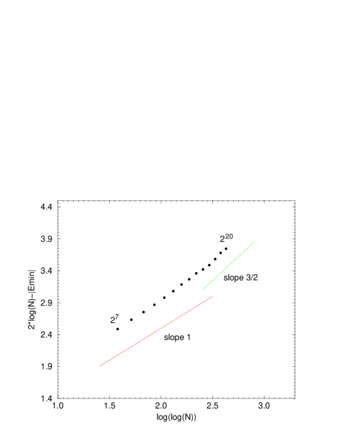
FIG. 10.: Zero temperature limit: finite size corrections to the minimal energy. Plotted is $2l-|V_{min}|$ versus $\ln l$ ($l=\ln N$)

Next, we have plotted the distribution of $V_{min}$ in Fig. 11 and compared with the prediction of the RG for the tails. Here also the agreement is satisfactory.

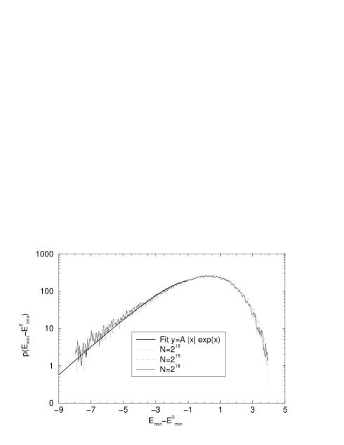
FIG. 11.: Distribution of $E_{min}$

Finally, we have plotted the “glass order parameter” $Y_{2}=\overline{\sum_{r}p_{r}^{2}}$ which is non zero when the system is dominated by a few states. It is consistent with a very slow convergence towards $Y_{2}=(1-T/T_{c})\theta(T_{c}-T)$ but clearly other forms cannot be ruled out.

FIG. 12.: Plot of $Y_{2}=\overline{\sum_{r}p_{r}^{2}}$ as a function of temperature for different system sizes $L=2^{N}$

V Relations with Liouville and Sinhgordon models

In this Section we describe the relation between the problem of the particle in the log-correlated random potential and the Liouville and sinh-Gordon models. Exact results on the sinh-gordon model are compatible with (and also point out towards) the existence of the transition at $\beta=\beta_{c}$.

A Relations with the sinh-Gordon model in $d=2$ and $d=1$

Let us start with the correspondence with the sinh-Gordon model. Although less direct, it is also simpler to analyze, as the model does not contain subtle boundary conditions problems. The interest of the connexion is that the sinh-Gordon model is integrable in $d=2$ and $d=1$ (Boundary sinh-Gordon) [59, 60, 61].

The connexion requires introducing a slightly different version of the initial problem, defined by the partition function:

$$Z_{sh}[V]=Z[V]+Z[-V]=\sum_{\bf r}(e^{-\beta V({\bf r})}+e^{\beta V({\bf r})})$$ (94)

which corresponds to a particle in a random potential which can explore both $V({\bf r})$ and $-V({\bf r})$. A physical realization would be a particle with an Ising spin in a random field. As it turns out the physics of this disordered model is very similar to the original problem. At low temperature, it is now related to the distribution of the minimum of $-|V({\bf r})|$.

We define the generating function of this model $G_{sh}(x)=\left<\exp(-\mu Z_{sh}[V])\right>$, with $\mu=e^{\beta x}$, which is related to the distribution of the free energy of the particle. In the continuum limit and in $d=2$, it can be rewritten as:

$$G_{sh}(x)=H_{sh}[\mu]=\int DVe^{-S_{sh}[V]}$$ (95)

$$S_{sh}[V]=\int_{-\infty}^{+\infty}\int_{-\infty}^{+\infty}dxdy\left(\frac{1}{8\pi\sigma}(\nabla V)^{2}+2\mu\cosh(\beta V({\bf r}))\right)$$ (96)

i.e the partition function of the sinh-Gordon model in $d=2$. Similarly, the $d=1$ version of our model is related to the well studied boundary sinh-Gordon model [60] defined as:

$$G_{shB}(x)=H_{shB}[\mu]=\int DVe^{-S_{shB}[V]}$$ (97)

$$S_{shB}[V]=\int_{0}^{+\infty}dy\int_{0}^{L}dx\biggl{(}\frac{1}{4\pi\sigma}(\nabla V)^{2}$$ (98)

$$\quad\quad\quad\quad\quad\quad\quad\quad\quad\quad\quad\quad+2\mu\cosh(\beta V(x,0))\biggr{)}$$ (99)

Indeed one has, as required, that $(V(x,0)-V(x^{\prime},0))^{2}\sim 4\sigma\ln\frac{|x-x^{\prime}|}{a}$ at large $|x-x^{\prime}|$, and one only studies (boundary) observables defined at $y=0$.

In the limit of $\beta=+\infty$ one has in both case:

$$G_{sh}(x) = \text{Proba}(x<\text{min}(V_{r},-V_{r}))$$ (100)

$$= \text{Proba}(x<-\text{max}_{r}|V_{r}|)$$ (101)

and thus the (properly discretized) partition function of the (boundary) sinh-Gordon model becomes related, in that limit, to the distribution function of the maximum of the set of positive random variables $|V({\bf r})|$. The results described in the previous Sections about the statistics of extrema of such variables imply that some transition must occur as a function of $\beta$ corresponding to a related “change of behaviour” in the sinh-Gordon and boundary sinh-Gordon models as well. This is a prediction, as we are not aware of such a change of behaviour at $\beta=\beta_{c}$ being mentionned in the literature. As we now discuss, examination of known results is perfectly compatible with the transition at $\beta=\beta_{c}$.

Let us first describe the known exact results both in $d=2$ and $d=1$. The extensive free energy of the bulk sinh-Gordon model is defined as:

$$f_{sh}=\lim_{L\to+\infty}-L^{-2}\ln G_{sh}$$ (102)

where the model defined in (96) is considered in finite size $L$. The model is studied usually using the field $\phi=V\sqrt{2/\sigma}$, the nonlinear term being $2\mu\cosh(\beta V)=2\mu\cosh(b\phi)$ and its free energy depends on the single variable $b=\beta\sqrt{\sigma/2}=\beta/\beta_{c}$, where $\beta_{c}=\sqrt{d/\sigma}$ is dimension dependent. Using the variable $b$, its exact expression, proposed in Ref. [59], reads when explicited [62]:

$$f_{sh}(\mu)=C_{2}(b)\mu^{\frac{1}{1+b^{2}}}$$ (103a)

$$C_{2}(b)=\frac{2\pi}{\left(\Gamma[\frac{1}{2+2b^{2}}]\right)^{2}\left(\Gamma[1+\frac{b^{2}}{2+2b^{2}}]\right)^{2}\sin(\frac{b^{2}\pi}{1+b^{2}})}$$ (103b)

$$\quad\quad\quad\quad\quad\quad\quad\quad\times\left(\frac{\pi\Gamma[1+b^{2}]}{-\Gamma[-b^{2}]}\right)^{\frac{1}{1+b^{2}}}$$ (103c)

These results are a priori only valid for $b<1$ ($|b|<1$), as they were obtained in [59] from an analytical continuation of the sine-Gordon model (performing $\mu\to-\mu$ and $b^{2}\to-b^{2}$, $M$ being the soliton mass). The constant $\mu$ was defined in the continuum model by fixing the normalization of the field $<\cos(b\phi({\bf r}))\cos(b\phi{\bf r}^{\prime})>=\frac{1}{2}|x-y|^{-4b^{2}}$ of the sine-Gordon model.

The $d=1$ version corresponds to the boundary sinh-Gordon model usually studied using the $\phi=V/\sqrt{\sigma}$ and $2\mu\cosh(\beta V)=2\mu\cosh(b\phi)$, with again $b=\beta/\beta_{c}$ ($\beta_{c}=1/\sqrt{\sigma}$). The analogous expression for the free energy reads, from [60]:

$$f_{shB}(\mu)=\lim_{L\to+\infty}-L^{-1}\ln G_{shB}=C_{1}(b)\mu^{\frac{1}{1+b^{2}}}$$ (104)

$$C_{1}(b)=\frac{1}{8\pi^{3/2}}\Gamma\left[\frac{1+2b^{2}}{2+2b^{2}}\right]\Gamma\left[\frac{-b^{2}}{2+2b^{2}}\right]\left(-\frac{2\pi}{\Gamma[-b^{2}]}\right)^{\frac{1}{1+b^{2}}}$$ (105)

Let us now comment on these results. The power law dependence in $\mu$ of the free energy is just the naive dimensional result $\sim\mu^{\frac{1}{1+b^{2}}}$ in both cases. This result should hold for $\beta<\beta_{c}$. However, there is clearly, in both $d=2$ and $d=1$ cases, a singularity as $\beta\to\beta_{c}^{-}$ as the amplitude $C(b)$ diverges as $b=\beta/\beta_{c}\to 1^{-}$. This is thus in perfect agreement with the existence of a phase transition in the particle model. In the sinh-Gordon model itself, we do not expect strictly speaking a phase transition, as the model is massive both below and above $b=1$, however we do expect some “change of behaviour”, which may be related to a change of nature of the excitations around the ground state. This is not ruled out by exact results [63] as it clearly comes here from the physical mass acquiring a nontrivial dependence in the bare mass parameter $\mu$ (contrarily to sine-Gordon model, for sinh-Gordon model there is no presently known exact solution of a lattice version).

Let us now interpret these results for our model. They mean that the generating function $G_{sh}(x)$ of the free energy distribution, with $\mu=e^{\beta x}$, takes indeed the form of a traveling wave:

$$G_{sh}\sim\exp\left(-L^{2}C_{d}\left(\frac{\beta}{\beta_{c}}\right)\mu^{\frac{2}{(1+\frac{\beta}{\beta_{c}})^{2}}}\right)=g(x+cl+\gamma)$$ (106)

with $l=\ln L$ and a velocity:

$$c=\frac{d}{\beta}+\sigma\beta$$ (107)

This is exactly the velocity given by the KPP equation for the particle model, in the high temperature phase. It also yields a front $g(y)=\exp(-e^{ay})$ with $a=\frac{\beta}{1+(\beta/\beta_{c})^{2}}$ and $\gamma=\frac{\beta}{1+(\beta/\beta_{c})^{2}}\ln C_{d}(\beta/\beta_{c})$. This form however should be taken with caution as strictly speaking formula (106) is valid only in the limit where $L$ goes to infinity first (at fixed $\mu=e^{\beta x}$). It should be compared with the asymptotic behaviour of the front in the region of large positive $y$. We expect universality in the other region of the front (of very negative $y$ i.e. $x<<cl$) and exact knowledge about this region would be equivalent to exact knowledge of the sinh-Gordon model at finite size, which is not yet available.

The physics of the problem of the particle in the random potential leads us to conjecture that the 2d sinh-Gordon model (as well as the boundary sinh-Gordon model) will exhibit a change of behaviour, the algebraic $\mu$-dependance of its free energy will freeze for $\beta\geq\beta_{c}$, which corresponds to the low temperature glassy phase of the particle model. We thus expect:

$$f_{sh}(\mu)\sim\mu^{\alpha}$$ (108a)

$$\alpha=\frac{1}{1+(\beta/\beta_{c})^{2}}\qquad \beta<\beta_{c}=\sqrt{d/\sigma}$$ (108b)

$$\alpha=\frac{1}{2}\qquad \beta>\beta_{c}=\sqrt{d/\sigma}$$ (108c)

and presumably log corrections (at least at $\beta=\beta_{c}$, and maybe for all $\beta>\beta_{c}$).

This is confirmed by a renormalization group analysis directly on the Sinh-Gordon and Liouville models discussed below.

B Relation with the Liouville model in $d=2$

The relation between our original model (1) of the particle in the random potential and the Liouville model proceeds via the generating function:

$$G(x) = \left<\exp(-e^{\beta x}Z[V])\right>_{V}$$ (109)

$$= \left<\exp(-\sum_{\bf r}e^{\beta(x-V({\bf r}))})\right>_{V}$$ (110)

which encodes the full probability distribution of the free energy of the particle. In the case of the $d=2$ potential with logarithmic correlations it is identical to the partition function of a Liouville model, which one can write either on the original lattice or in the continuum (with UV and IR cutoffs $a$ and $L$) as ($\mu=e^{\beta x}$) :

$$G(x)=H[\mu]=\int DVe^{-S[V]}$$ (111)

$$S[V]=\int d^{2}{\bf r}\left(\frac{1}{8\pi\sigma}(\nabla V({\bf r}))^{2}+\mu~{}e^{-\beta V({\bf r})}\right)$$ (112)

where the functional integral is normalized such that $H[\mu=0]=1$ (equivalently one redefines $H[\mu]\to H[\mu]/H[\mu=0]$). We call it the Liouville Model (LM) to distinguish it from the continuum Liouville field theory LFT whose definition is recalled below. A relation also exists between the correlation functions of the Gibbs measure and some correlation functions in the Liouville model:

$$<p({\bf r}_{1})..p({\bf r}_{n})>=\int_{\mu>0}\mu^{n-1}e^{-\beta(V({\bf r}_{1})+...V({\bf r}_{n}))}e^{-S[V]}$$ (113)

Strictly speaking the model (112) above is not well defined because of the zero mode $V({\bf r})\to V({\bf r})+w$ and must be complemented with boundary conditions. In the particle problem studied here we have chosen periodic boundary conditions with the additional constraint $\sum_{\bf r}V({\bf r})=0$ to pin the zero mode.

On the other hand, many results are known for the (related) continuum Liouville field theory (LFT), of great interest in quantum gravity [64, 65, 66, 67, kazakov]. It is usually defined on a arbitrary genus $h$ manifold with background metric $g$ and associated curvature $R$ by the action [68]:

$$S_{LFT}=\int d^{2}x\left(\frac{1}{4\pi}(\partial_{a}\phi)^{2}+\mu e^{2b\phi}+\frac{Q}{4\pi}R\sqrt{g}\phi\right)$$ (114)

in conventional notations, with $\phi=-V/\sqrt{2\sigma}$ and $b=\beta/\beta_{c}$. The (standard) choice is $Q=b+1/b$ for which the theory is critical and has local conformal invariance (with a central charge $c_{L}=1+6Q^{2}=25+c$) [68]. It can also be formulated as the theory of (liquid) random surfaces [67, 69] e.g. as random triangulations. There one defines the total area $A=\int_{\bf r}e^{-2b\phi(r)}$ which is nothing but the partition function $A=Z[V]$ of the particle problem, and studies the distribution ${\cal Z}(A)\sim e^{-\mu_{c}A}A^{\gamma_{\text{string}}-3}$ which is nothing but $P(Z)$.

The particle model allows us to make precise statements on the Liouville model defined above. The LFT allows for exact calculations (e.g. of correlation functions) and in principle one could hope to translate those in the particule model (Gibbs measure correlations). The relation between the two however is rather subtle. For instance, the boundary conditions chosen in the particle problem would correspond to Liouville on a torus $h=0$, except that the additional pinning condition spoils it. We will thus not explore here all these intricacies but give a few general remarks, mostly about the behaviour of the Liouville model under coarse graining.

First we know that $G_{l}(x)$ satisfies a RG equation of the KPP type. Thus upon coarse graining (i.e as a function of $l=\ln(L/a)$ see Section III) the Liouville model partition function satisfies a KPP non linear RG equation. The corresponding front velocity gives the scaling of the partition function with $\mu$. The glass transition, with freezing of the front velocity, corresponds exactly in the Liouville model to the transition between two regimes (the so-called $c=1$ barrier in the LFT):

(i) weak coupling Liouville: $b=\beta/\beta_{c}<1$. In that regime there is no problem to define a continuum limit. The KPP non linear RG front solution of velocity $c(\beta)=2(\frac{1}{\beta}+\frac{\beta}{\beta_{c}^{2}})\equiv c(b)$ yields $G_{l}(\mu)\sim\mu^{1/(1+b^{2})}$ and in the Liouville model the scaling dimensions are the one obtained by naive dimensional counting. e.g. :

$$\mu\int d^{2}{\bf r}e^{-\beta V({\bf r})}=\mu e^{\ln Z[V]}\sim\mu L^{\beta c(\beta)}=\mu L^{2(1+b^{2})}$$ (115)

In the LM only one of the two branches (deduced by $b\to 1/b$) is selected as $l\to+\infty$.

The regime $b\leq 1$ is the one where the continuum LFT is well defined: there the role of the $Q$ term in (114) is to shift the conformal dimension of the fields $e^{2\alpha\phi}$ to $\Delta(\alpha)=\alpha(Q-\alpha)$ (while the naive power counting dimensions in the LM are $\Delta(\alpha)=-\alpha^{2}$, see above) which renders the Liouville term $\int e^{2b\phi}$ exactly marginal (and thus the theory critical). It was argued in [13] that the LFT gives the correlations of the Gibbs measure, the operator $p({\bf r})$ (eq. (2)) corresponding to the Liouville field $e^{2b\phi}$ (and is thus of conformal dimension $\Delta(b)=1$ (i.e $p({\bf r})\sim L^{-2}$). A hint in favor of this conjecture was that the corresponding LFT conformal dimensions of the composite fields $p({\bf r})^{q}\sim e^{2qb\phi}$ is simply $\Delta(q)=q(1+b^{2}-b^{2}q)$ which correctly reproduces the multifractal spectrum:

$$\int d^{2}{\bf r}~{}p({\bf r})^{q}\sim L^{2(1-\Delta(q))}$$ (116)

given in [12] and Section VI (in the weak disorder regime $q<q_{c}$). This is not a very strong test since the same multifractal spectrum can also be obtained within the LM model by considering the dimension of the normalized Gibbs measure (rather than the unnormalized one $e^{-\beta V}$). Indeed the effect of the $Q$ term is to shift:

$$e^{2bq\phi}\to L^{2bqQ}e^{2bq\phi}\sim Z[V]^{-q}e^{2bq\phi}$$ (117)

To convincingly establish the conjecture of [13] the effect of the additional $Q$ term should be checked on the many point correlations [68], where it is rather more subtle, and further investigation is needed. In particular, the RG described here suggests by extension that the Gibbs measure correlations (or at least some limits of them) should also be computable within the DPCT model. This suggests a direct relation between LFT and DPCT, a check of which would be of great interest. Note also that a critical model, which mimics the effect of the $Q$ term (as adding an average value to $\phi$ [68]) is studied in Appendix D.

(ii) strong coupling Liouville: $b=\beta/\beta_{c}>1$. This corresponds to the glass phase for the particle which, interestingly, has a non trivial structure. As is well known there are serious difficulties in defining the continuum LFT in that regime. Using what we know from the particle problem we can gain some idea of what happens in the Liouville theory. First let us note that since $G(x)$ is such that for $\beta=+\infty$ and fixed $L$ it is equal to the distribution function of the minimum of the set of $V({\bf r})$:

$$G(x)=\text{Proba}(x<\min_{{\bf r}}V({\bf r}))$$ (118)

The (infinitely strong coupling) Liouville model can be recast as an extremal statistics problem in that limit. The partition sum $Z[V]$ of the particle model being dominated, for $b>1$ by a few regions of space where $V({\bf r})\sim V_{min}$ (with little dependence in $\beta$, i.e the Liouville wall become a hard wall for all $\beta<\beta_{c}$ with thickness of order $O(1)$) we expect this spatial heterogeneity to show up in LM as well. From what we have learned in previous Sections we know that upon coarse graining the following effective Liouville model action $S_{eff}$ is generated:

$$G_{l}(x)=H_{l}[\mu]=\int D\tilde{V}<e^{-S[\tilde{V},z]}>_{P(z)}$$ (119)

$$S_{eff,l}[V]=\int d^{2}{\bf r}\left(\frac{1}{8\pi\sigma}(\nabla\tilde{V}({\bf r}))^{2}+z({\bf r})e^{-\beta\tilde{V}({\bf r})}\right)$$ (120)

i.e a new field $z({\bf r})$ is dynamically generated, and has short range correlations but has a broad power law distribution:

$$P(z)dz\sim z^{-1+\frac{1}{b}}$$ (121)

while $\tilde{V}\equiv V^{>}$ is the smooth field introduced in (17). For $b<1$ this dynamically generated local field can be averaged out without changing significantly the action (note that even for $b<1$ it changes properties of operators $e^{-q\beta V}$ for $q>q_{c}$) while for $b>1$ it changes crucially the physics. One can define the effective Liouville potential $U[V]$ for the smooth field $\tilde{V}$ after averaging over the $z$ field as:

$$U_{l}[\tilde{V}]=-\ln<\exp(-ze^{-\beta\tilde{V}})>_{P_{l}(z)}=-\ln G_{l}(x=-\tilde{V})$$ (122)

the bare Liouville potential being $U[V]=\mu~{}\exp(-\beta V)$. We can now use the front solution of the KPP equation (i.e the scaling region in the large $L/a$ limit) described in previous Sections. For $b<1$, since $<z>_{P(z)}<+\infty$ we have that for large $V$

$$U_{l}[V]\approx c\mu e^{2(1+b^{2})l}\exp(-\beta V)$$ (123)

and thus the coarse grained potential is similar to the bare one. However, for $b>1$ one has for large $V$

$$U_{l}[V]\approx c\mu e^{4l}V\exp(-\beta V)$$ (124)

because of the broad distribution of the $z$ field.

Since the $z({\bf r})$ are highly heterogeneous on short scales it is not surprising that a continuum limit is hard to obtain for $b>1$. These heterogeneities are linked to the structure of the glass phase reminiscent of replica symmetry breaking. It is tempting to conjecture that it may also be related to the branched polymer structure which appear in LFT for $b>1$, i.e beyond the $c=1$ barrier [67], or to the spike instability [69] of fluid membranes.

Furthermore, let us notice that the LFT theory at $b=1$ is known to have two marginal operators whose dimensions are degenerate $e^{2b\phi}$ and $\phi e^{2b\phi}$. This is in exact parallel with the behaviour of the KPP front solution, which develops at $b=1$ two degenerate linear eigenmodes $\exp(-\beta V)$ and $V\exp(-\beta V)$.

Thus we have seen that the Coulomb gas RG can be used to understand the behaviour of the Liouville model. A scenario is obtained where for $b\geq 1$ new short scale degree of freedom are generated (short scale instability). Averaging over these changes the effective Liouville potential. The parallel with the particle model suggests that the short scale instability in Liouville may be related to the generation of strong inhomogeneities in the Gibbs measure $p({\bf r})$, analogous to structures discussed in the context of replica symetry breaking. Thus, if the mapping onto the LFT is confirmed it suggests to also investigate RSB type effects in strong coupling LFT.

C Direct renormalisation group analysis of sinh-Gordon and Liouville models and traveling waves

Let us now illustrate how one can see explicitly the freezing of the free energy exponent in the strong coupling phase from renormalisation group approaches directly on the sinh-Gordon and Liouville models. Such functional RG methods have been applied to study the analogous problem [30] of the wetting of an interface of height $V$. Related exact RG methods, with various truncation schemes, have also been applied to the Liouville model, and in the context of quantum gravity to the LFT [70]. In all cases we will illustrate how the main physics lies in the selection mechanism for the traveling wave solutions of the non linear RG equation.

FIG. 13.: Liouville wall moving under RG as a travelling wave. Represented is $U[V]$ on the negative $V$ side, of original form $U[V]=e^{-\beta(V-x)}$ and also (dashed line) $G(x)=\exp(-U[V])$. Both move under RG forming a travelling front, whose velocity determines the “free energy” exponent. For sinh-Gordon a second, mirror image wall is also moving symmetrically towards $0$. Freezing in the front velocity occurs at and below the transition at $\beta=\beta_{c}$.

The study proceeds as follows. We consider

$$G(x)=H[\mu=e^{\beta x}]=\int DVe^{-S[V]}$$ (125)

with $$S[V]=\int d^{2}{\bf r}\left(\frac{1}{8\pi\sigma}(\nabla V({\bf r}))^{2}+U[V]\right)$$ (126)

One can perform a Wilson RG analysis (or if one prefers a suitably truncated exact RG analysis), and one finds in $d=2$ the flow for the local part $U_{l}[V]$ as:

$$\partial_{l}U=2U+\sigma U^{\prime\prime}+O(U^{2})$$ (127)

There may also be corrections to $\sigma$ to $O(U^{2})$ (in the Sinh-Gordon model), but we focus for now on the RG to linear order. Let us recall that the initial condition is $U_{l=0}[V]=\mu e^{-\beta V}$ for Liouville and $U_{l=0}[V]=\mu e^{-\beta V}+\mu e^{\beta V}$ for sinh-Gordon, and that we are interested in the small $\mu$ limit. In this limit the initial condition corresponds to a a very wide well $U[V]$ (e.g. in the sinh-Gordon model) with a very small curvature $U^{\prime\prime}[0]$. To obtain the free energy exponent as $\mu\to 0$, one simply iterates the RG until $U_{l}^{\prime\prime}[0]\sim O(1)$ at a scale $l^{*}=\ln(L^{*}/a_{0})$ (more precisely $U_{l}^{\prime\prime}[0]\sim 1/(\sigma a_{0}^{2})$ where $a_{0}$ is the bare UV cutoff of the model). At this scale, the free energy is $O(1)$, as can be estimated from gaussian fluctuations (straightforwardly at least in the SG model) and thus the initial free energy is:

$$F\sim A_{d}(\beta)\left(\frac{L}{L^{*}}\right)^{2}$$ (128)

Remarkably, it is now possible to use what we learned in the previous Sections and demonstrate the “freezing” transition at $\beta=\beta_{c}$ (corresponding to the glass transition for the particle) simply from the RG to this order. Indeed the solution of the truncated equation is:

$$U_{l}[V]=e^{2l}\frac{1}{\sqrt{4\pi\sigma l}}\int dV^{\prime}\exp\left(-\frac{(V-V^{\prime})^{2}}{4\sigma l}\right)U_{l=0}[V]$$ (129)

A straigthforward conclusion would then be that the exact solution corresponding to Liouville is:

$$U_{l}[V]=\mu e^{(2+\sigma\beta^{2})l}e^{-\beta V}$$ (130)

and similarly for the sinh-Gordon:

$$U_{l}[V]=2\mu e^{(2+\sigma\beta^{2})l}\left(e^{-\beta V}+e^{\beta V}\right)$$ (131)

since $\exp(\pm\beta V)$ are exact eigenvectors of the linear RG equation for any $\beta$. From (128) this immediately yields the “naive dimensional” result for the free energy

$$F\sim L^{2}\mu^{\frac{1}{1+(\beta/\beta_{c})^{2}}}$$ (132)

with $\beta_{c}=\sqrt{2/\sigma}$. As we know from the above exact result this is correct for $\beta<\beta_{c}$. Note how the potential $U_{l}[V]$ evolves. Using the notation $\mu=e^{\beta x}$ (natural from our extremal statistics interpretation) it forms a “Liouville wall”, which can be seen as a “front solution” moving as $\exp(-\beta(V-x-cl))$ towards $U=0$ (and in the sinh-Gordon model there are two symmetric walls moving towards $U=0$ and reaching it at $l=l^{*}$). The Liouville front velocity is:

$$c=\frac{2}{\beta}+\sigma\beta$$ (133)

which plotted as a function of $\beta$ is the famous parabola, such that two values of $\beta$ corresponds to the same $c$, which is also a well known property of Liouville theory.

As we now show, (130) is incorrect for $\beta\geq\beta_{c}$. This is so for a subtle reason, as apparently the statement that $\exp(-\beta V)$ is an exact eigenvector of the linear RG (and of (129)) cannot fail ! However, by now we are well used to fronts: in fact we have encountered exactly the same equation in our previous solution of the REM model via RG ($h_{l}(x)$ in (73) is identical to $U_{l}(V)$ in (129)). To describe correctly the bare Liouville (or equivalently the Sinh-Gordon) model one should generalize the initial condition $U_{l=0}[V]$, still assuming that $U_{l=0}[V]\sim\exp(-\beta(V-x))$ for $V\gg x$ ($x$ here is very negative corresponding to a small $\mu$). Then one can use the saddle point method to estimate (129) as was done in (73) to evaluate $h_{l}(x)$ and one discovers that for $\beta>\beta_{c}$ the velocity freezes into:

$$c=2\sqrt{2\sigma}$$ (134)

which yields a free energy

$$F\sim L^{2}\mu^{\frac{1}{2}}$$ (135)

instead of the naive dimensional estimate, thus in agreement with our expectation for the SG model (108c). In addition we find that the decay of the renormalized potential $U_{l}[V]\sim e^{-\alpha V}$ is frozen at $\alpha=\beta_{c}$ for all $\beta>\beta_{c}$ consistent with (124).

What has happened is that although $U_{l=0}[V]=\exp(-\beta(V-x))$ is indeed formally an exact eigenvector, it is dynamically unstable, i.e if one chooses another function with the same large positive $V-x$ behaviour one gets a different velocity (which is not the case for $\beta<\beta_{c}$). It is easy to see that the choice $U_{l=0}[V]=\exp(-\beta(V-x))$ exactly for all $V$ does not make sense for $V\to-\infty$. Indeed it is immediately spoiled by the slightest amount of coarse graining (as would appear also by considering the non linearities in the RG equation). The simplest way to see it is to notice that the coarse grained potential:

$$\tilde{U}[V]=-\ln\left(\int dv\exp(\left[-\mu e^{-\beta(V+v)}\right]-\frac{v^{2}}{2s})\right)$$ (136)

does not grow as $\sim\exp(-\beta V)$ for large negative $V$ but much slower as $\sim V^{2}$. To illustrate further the point let us consider the initial condition:

$$U_{l=0}[V]=\frac{e^{-\beta(V-x)}}{1+e^{-\beta(V-x)}}$$ (137)

It behaves as $e^{-\beta(V-x)}$ for large positive $V-x$ (and thus corresponds to the Liouville model) but goes to $1$ on the other side. For $\beta=+\infty$ it is easy to compute $U^{\prime\prime}_{l}[V=0]$ from (129) since $U_{l=0}[V]=\theta(x-V)$. One finds:

$$U^{\prime\prime}_{l}[V=0]\sim e^{2l-\frac{x^{2}}{4\sigma l}}$$ (138)

and thus one has that $l^{*}$ defined above is such that:

$$cl^{*}=x\qquad c=2\sqrt{2\sigma}$$ (139)

This is in fact valid for all $\beta>\beta_{c}$ as was shown in detail in previous sections.

Thus the freezing transition can be obtained from the linearized (i.e lowest order) RG equations, using only elementary insight from coarse graining or the existence of higher order non linear terms. It provides an interesting example where the naive dimensions hold in some regime but are modified in another. Of course, as we have seen in Section III D from the study of fronts, to really establish the transition and determine the universality class one needs to consider higher order non linearities in (127) which goes beyond this paper. For the LFT in quantum gravity the reader can find some exact functional RG studies in Ref. [70]. Although not discussed in this reference, the non linear RG there seems to also exhibit traveling front solutions, whose physics may be important in understanding the problem of the $c=1$ barrier.

VI Critical Dirac fermions in a random gauge field

In this section we relate our RG study of the previous section to the study of the critical wave functions of 2D Dirac fermions in a random magnetic field. We first confirm the results of [14] for the multifractal spectrum, and obtain their finite size corrections. Then we study the transition from the weak disorder to the strong disorder phase, related to the glass transition for the particle, and find that the strong disorder phase has a new and non trivial structure, leading to what we call quasi-localized eigenstates.

A Critical wave function of 2D random Dirac

Let us first recall the problem of a massless two dimensional Dirac fermion in a static random magnetic field [12, 14, 33]. This model, and its non abelian generalizations, has received a lot of attention in connection with the integer quantum Hall effect transitions with disorder. As discussed in [25] two dimensional Dirac fermions can experience three generic types of disorder: random gauge, random mass and random potential. Random gauge disorder is believed to be a line of fixed points in this general model and is still not yet fully understood. Here we address only the random gauge disorder model of hamiltonian:

$$H=\sigma_{\mu}\left(iv_{F}\partial_{\mu}-A_{\mu}({\bf r})\right)$$ (140)

where the $\sigma_{1,2}$ are the $2$x$2$ Pauli matrices and $\mu=1,2$ (we set the Fermi velocity $v_{F}=1$ from now on). The random magnetic field ${\bf B}$ corresponding to the gauge potential ${\bf A}$ is chosen to be gaussian with mean value $\overline{{\bf B}({\bf r})}=0$. The type of correlations studied here correspond to the most interesting case where the gauge potential has short range correlations. In the Coulomb gauge, we can introduce the scalar potential $\phi$ such that $A_{\mu}=\epsilon_{\mu\nu}\partial_{\nu}\phi,B({\bf r})=-\partial_{\mu}^{2}\phi({\bf r})$. The gaussian distribution of $\phi({\bf r})$ is thus given by

$$P[\phi]=cte\times e^{-\frac{1}{4\pi g}\int_{{\bf r}}(\partial_{\mu}\phi({\bf r}))^{2}}$$ (141)

where $g$ parametrises the strength of the random magnetic field $B$. The correlator of the function $\phi({\bf r})$ is thus:

$$\overline{(\phi({\bf r})-\phi({\bf r}^{\prime}))^{2}}\sim 2g\ln\frac{|{\bf r}-{\bf r}^{\prime}|}{a}$$ (142)

In this model, the wave functions at energy $E$ are localized for all energies other than the critical energy $E=0$. We restrict our study to the $E=0$ critical eigenstate, which satisfy:

$$H\Psi_{0}({\bf r})=0$$ (143)

For a system of finite size $L$ with appropriate boundary conditions there are two independent normalized solutions of (143): the first one can be written $\Psi_{0,1}({\bf r})=(\Psi_{0}({\bf r}),0)$ with:

$$\Psi_{0}({\bf r})^{2}=\frac{e^{-2\phi({\bf r})}}{\sum_{\bf r}e^{-2\phi({\bf r}^{\prime})}}$$ (144)

the second one being $\Psi_{0,2}({\bf r})=(0,\tilde{\Psi}_{0}({\bf r}))$ where $\tilde{\Psi}_{0}({\bf r}))$ is given by (144) changing $\phi({\bf r})\to-\phi({\bf r})$. We denote $\sum_{\bf r}$ having in mind either a discrete problem, or a continuous problem with some short scale cutoff $a$.

B participation ratios and multifractal spectrum

Thus in a given configuration of disorder $\phi({\bf r})$ the quantum probability $|\Psi_{0}({\bf r})|^{2}$ is identical to the Gibbs probability $p({\bf r})$ defined in (2) for the particle in the logarithmically correlated random potential $V({\bf r})$ with the correspondence:

$$|\Psi_{0}({\bf r})|^{2}=p({\bf r})$$ (145)

$$2\phi({\bf r})=\beta V({\bf r})$$ (146)

and thus the model depends on a single parameter $g=\frac{1}{2}\beta^{2}\sigma$. As we have discussed in previous Sections the particle in the logarithmically correlated random potential undergoes a transition at $\beta_{c}=\sqrt{2/\sigma}$ at which its Gibbs measure changes from being dominated by many sites (high $T$ phase) to being dominated to a few sites (low $T$ phase). Thus in the quantum problem we expect a transition at:

$$g=g_{c}=1$$ (147)

with a weak disorder phase for $g<1$ and a strong disorder phase for $g>1$. In the weak disorder phase the quantum probability (and thus observables such as the mean squared position fluctuations $<r^{2}>-<r>^{2}$) is delocalized ($<..>$ means averages over $\Psi_{0}$). In the strong disorder phase the quantum probability is more concentrated, but it cannot be called localized in the usual sense (of an exponential decay around a single center) and in fact both phases have rather peculiar properties.

Properties of wave functions can be described by the inverse participation ratios defined from the normalized wave function $\Psi_{0}({\bf r})$ in a system of size $L$ by

$$R_{q}(L)=\int d^{2}{\bf r}|\Psi_{0}({\bf r})|^{2q}=\int d^{2}{\bf r}~{}\left(p({\bf r})\right)^{q}$$ (148)

At a very qualitative level, the nature of the eigenfunction can be inferred from the scaling behaviour of the inverse participation ratio with the system size $L$ : for an exponentially localized state $R_{q}(L)$ scales [71] as $R_{q}(L)\sim\text{const}$ for all $q>0$, while for a plane wave delocalized state we get $R_{q}(L)\sim L^{-2(q-1)}$. In addition to the localized and delocalized states, there exist states such that $\tau(q)=-\ln R_{q}(L)/\ln L$ is a non linear function of $q$: they correspond to multifractal wave functions whose moments cannot be described by a single length as usual but rather by a spectrum of exponents. Here, as in [14], we also find intermediate multifractal behaviour.

To compute the finite size inverse participation ratios we can use the information of previous Sections since:

$$s_{q}(L)=-\ln R_{q}(L)=-\ln Z_{q^{2}g}+q\ln Z_{g}$$ (149)

where we have defined $Z_{g}=Z(\beta=\sqrt{2g/\sigma})$ where $Z(\beta)$ is the partition function for the particle at inverse temperature $\beta$. In particular we will be interested in the multifractal asymptotic scaling exponent $\tau(q)$ defined by

$$\tau(q)=\lim_{L\to\infty}\frac{s_{q}(L)}{\ln L}$$ (150)

These exponents were computed previously in [14] using the REM approximation. Here we use our RG results and also obtain finite size corrections. Note that these correspond to properties of $\Psi_{0}$ defined above and could be changed if other boundary conditions were used.

From the previous Sections we obtain:

$$\ln Z_{g}=2(1+g)\ln L+\Delta_{g} ,g<1$$ (151a)

$$\ln Z_{g}=(\sqrt{g}(4\ln L-\frac{1}{2}\ln(\ln L))+\Delta_{g} ,g=1$$ (151b)

$$\ln Z_{g}=(\sqrt{g}(4\ln L-\frac{3}{2}\ln(\ln L))+\Delta_{g} ,g>1$$ (151c)

where $\Delta_{g}$ is a sample dependent variable of order $O(1)$ with a $g$ dependent distribution (whose tails we have characterized previously). From there we obtain $s_{q}(L)$, which have different behaviours in the two phases.

(i) weak disorder phase

For $g<1$ we find, denoting $q_{c}=\frac{1}{\sqrt{g}}$ :

$$s_{q}(L)=2(q-1)(1-gq)\ln L+A_{q,g}$$

$$\qquad\qquad\qquad\qquad\qquad\qquad\qquad\qquad\text{for }|q|<q_{c}$$

$$s_{q}(L)=\frac{2}{\sqrt{g}}(1-\text{sgn}(q)\sqrt{g})^{2}\ln L+\frac{1}{2}\ln\ln L+A_{q,g}$$

$$\qquad\qquad\qquad\qquad\qquad\qquad\qquad\qquad\text{for }|q|=q_{c}$$

$$s_{q}(L)=2q(1-\text{sgn}(q)\sqrt{g})^{2}\ln L+\frac{3}{2}|q|\sqrt{g}\ln\ln L+A_{q,g}$$

$$\qquad\qquad\qquad\qquad\qquad\qquad\qquad\qquad\text{for }|q|>q_{c}$$

where $A_{q,g}$ is a fluctuating part of order $O(1)$.

(ii) strong disorder phase

For $g>1$ we find:

$$s_{q}(L)=-2(q\sqrt{g}-1)^{2}\ln L-\frac{3}{2}q\sqrt{g}\ln\ln L+A_{q,g}$$ (153a)

$$\qquad\qquad\qquad\qquad\qquad\qquad\qquad\qquad\text{for }|q|<q_{c}$$ (153b)

$$s_{q}(L)=-\frac{1}{2}\ln\ln L+A_{q,g}\qquad\text{for }q=q_{c}$$ (153c)

$$s_{q}(L)=A_{q,g}\qquad\text{for }q>q_{c}$$ (153d)

$$s_{q}(L)=-2|q|\sqrt{g}\left(4\ln L-\frac{3}{2}\ln\ln L\right)+A_{q,g}$$ (153e)

$$\qquad\qquad\qquad\qquad\qquad\qquad\qquad\qquad\text{for }q<-q_{c}$$ (153f)

$$s_{q}(L)=-2\left(4\ln L-\frac{1}{2}\ln\ln L\right)+A_{q,g}\qquad\text{for }q=-q_{c}$$ (153g)

where $A_{q,g}$ is a fluctuating part of order $O(1)$.

The corresponding scaling exponents $\tau(q)$ are thus identical to the one found in [14] and in addition we have obtained their finite size corrections. In the weak disorder phase one for $q>0$:

$$\tau(q)=\left\{\begin{array}[]{lll}2(q-1)\left(1-\frac{q}{q_{c}^{2}}\right)&\text{ for }&q\leq q_{c}=\sqrt{\frac{1}{g}}\\ 2q\left(1-\frac{1}{q_{c}}\right)^{2}&\text{ for }&q\geq q_{c}\end{array}\right.$$ (154)

which means a parabolic form with a termination point at $q=q_{c}$ as represented in the Fig. 14.

FIG. 14.: Multifractal spectrum in the weak disorder phase

In the strong disorder phase $g>1$, i.e when $q_{c}\leq 1$, the above expression becomes (for $q>0$):

$$\tau(q)=\left\{\begin{array}[]{lll}-2\left(1-\frac{q}{q_{c}}\right)^{2}&\text{ for }&q\leq q_{c}=\sqrt{\frac{1}{g}}\\ 0&\text{ for }&q\geq q_{c}\end{array}\right.$$ (155)

Since the inverse participation ratio does not scale with the system size $L$ for each integer $q$, one could naively conclude that it is the sign of a localized state (see however below).

As was discussed in [14] these results can be translated into spectrum for exponent $\alpha$. If one assumes that $p({\bf r})$ is of order $L^{-\alpha}$ in a number $L^{f(\alpha)}$ sites then the above spectrum is recovered if:

$$f(\alpha)=8\frac{(d_{+}-\alpha)(\alpha-d_{-})}{(d_{+}-d_{-})^{2}}$$ (156)

with $d_{\pm}=2(1\pm\sqrt{g})^{2}$ for $g>1$ and $d_{+}=8\sqrt{g}$, $d_{-}=0$ for $g>1$. It is easy to see that:

$$<(r-<r>)^{2k}>\geq L^{\max_{\alpha}((k+1)f(\alpha)-\alpha)}$$ (157)

showing that the eigenstate is never localized in the usual sense (exponential decay around a single center) since the exponent is always positive for large enough $k$. Since $\lim_{q\to\pm\infty}s_{q}(L)/q=\ln p_{max,min}$ one obtains that the maximum of the Gibbs measure $p_{max}=\max_{{\bf r}}p({\bf r})$ and the minimum behave for large $L$ as:

$$p_{max}\sim L^{-2(1-\sqrt{g})}(\ln L)^{-\frac{3}{2}\sqrt{g}}$$ (158)

$$p_{min}\sim L^{-2(1+\sqrt{g})}(\ln L)^{+\frac{3}{2}\sqrt{g}}$$ (159)

in the weak disorder phase.

C nature of the strong disorder phase: quasi-localization

Let us now concentrate on the case $g>1$. There, we know from previous Sections that the Gibbs measure of the particle is concentrated in a few sites. Thus from (146) the quantum probability $|\Phi_{0}({\bf r})|^{2}$ is also concentrated in a few sites, analogous to the RSB picture. This is a very peculiar type of eigenstate. Indeed if one computes the quantum average $<r^{2}>-<r^{2}>$ in a given sample, it has a finite probability to be of order $O(L^{2})$. Thus the eigenstate cannot be considered as localized in the usual sense. Since it is peaked around a few sites we call it “quasi-localized”. Around these centers the wavefunction decays fast enough to be normalizable. It would be interesting to investigate further the typical spatial decay of such eigenstates around their (multiple) centers, which we expect to be slower than exponential.

VII conclusion

In this paper we have studied the equilibrium problem of a particle in a random potential with logarithmic correlations, through exact bounds, numerical simulation, qualitative arguments and a renormalization group method that we have developed specifically for this problem. We have shown that it exhibits a glass transition at finite temperature $T_{c}=1/\beta_{c}>0$ in any dimension. This confirms earlier conjectures and allows for a more detailed study of the problem. The RG method allowed to obtain the universal features of the free energy distribution at low temperature. The relation to the problem of extremal statistic of correlated variables was investigated. It has been found that it exhibits universal finite size corrections, consistent with our numerical calculations.

Most interestingly, we found that this logarithmic model provides a particularly simple example (maybe the simplest) of a finite dimensional model - i.e with translationally invariant disorder correlations- such that the low temperature phase is non trivial. It is non trivial in the sense that in the thermodynamic limit $L\to+\infty$, there are, with a finite probability, several low lying states (i.e possible positions of the particle) with energy differences of order one, and separated in space by distances of order $L$. Thus the Gibbs measure at low temperature is dominated by “a few” spatially well separated states. Interestingly, this transition and this type of glass phase occurs only for logarithmically growing correlations, faster growth (e.g. as in Sinai model) yielding only a glass phase with single ground state dominance, while slower growth yielding only a high temperature phase.

Although oversimplified in some respect (it has no internal space) it does provide one example of a model where the usual droplet picture (which assumes dominance of a single ground state - or several related by a symmetry) does not apply. Rather, it provides one example where some features of the physics usually associated to RSB, namely dominance by a few states with exponential free energy distributions, can be explicitly exhibited. In fact, due to the finite dimensional correlations, there are some departures from the behaviour observed in the simplest prototype mean field models (such as the REM), as can be seen for instance from the free energy distribution which has more structure than a simple exponential. It would of course be interesting to explore further the additional features specific to finite dimensions.

Although the present model is already of obvious physical interest (in 2D it describes e.g. a single vortex in a random gauge XY model) its non trivial properties provide a motivation to search for models with more degrees of freedom and with similar features. One way to proceed would be to search for interface models via an internal dimensional expansion around the present model. The key feature however appears to be the marginality of the model, i.e the logarithmic growth of typical energy fluctuations. This corresponds to a fluctuation energy exponent $\theta=0$, i.e the situation where the temperature (i.e the entropy) is marginal in the RG sense. The droplet arguments indeed assume that $\theta>0$, consistent with the single ground state dominance (and activated behaviour typical of a zero temperature fized point where $T$ is formally irrelevant). In the situation $\theta=0$ one does expect more generally power laws with $T$ dependent exponents, reminiscent of mean field. It would thus be of great interest to similarly exhibit other non trivial marginal models (e.g. spin models with $\theta=0$) with similar features [72]. Spin models where (domain wall) excitations (in root mean square and in average) also scale logarithmically (as vortices in the random gauge XY model) are presumably good candidates.

On one hand we have developed a specific (Coulomb gas) renormalization group (RG) approach to describe the model. From the study of the resulting nonlinear (KPP) RG equation, we found explicitly that a freezing phenomenon occurs at the glass transition temperature, and that in the glass phase a broad (power law) distribution of fugacities develop - or equivalently exponential distribution of local free energy. It is different from more conventional perturbative RG (e.g. the one which was used to study the dynamics of this model) in the sense that the full distribution of probability is followed. This turns out to be crucial to describe the low temperature phase.

On the other hand, as we have discussed, two approximations of the present model, the REM approximation and the DPCT hierarchical version can both be solved using replica and do require considering the analytical continuation to $m\to 0$ of contributions of replica symmetry breaking saddle points [11].

This shows that a RG approach which is explicitly replica symmetric but allows to treat broad disorder distributions can be consistent with (approximate) approaches based on RSB saddle points [73]. We have illustrated this on the REM which can be recast in terms of non linear RG equations, with a freezing transition. In fact one of the striking property of the model is that the RG equations derived here are similar - to the order we have been working - to the one which hold for a continuous version of the DPCT problem, the branching process. In particular it indicates that both problem share the same universal finite size corrections.

We have also analyzed some connections in 2D (and via boundaries in 1D) between the model of the particle and the Liouville and Sinh Gordon models. The intensive free energy of the particle corresponds to the scaling dimension in these models with $b=\beta/\beta_{c}$. The glass transition corresponds to the weak to strong coupling transition at $b=1$. Beyond, corresponding to the glass phase, the scaling dimension freezes as we have also shown via a direct RG approach on these models. We have seen that under coarse graining an additional local field appears in the LM and SGM, with broad distribution, and corresponds to inhomogeneous configurations being generated (and broad fluctuations of the local area since the local partition function corresponds to local area).

The present study raises interesting issues to be explored concerning the relations with the continuum Liouville Field Theory (LFT). An outstanding question is whether the conjecture of [13] is correct for the correlations. Since we have obtained another result linking the problem to the DPCT, the direct comparison of the LFT and the DPCT remains to be studied. If it holds it means that the conformally invariant many point correlations can be related in some limits (large separations with fixed ratios $\ln r_{ij}/\ln r_{kl}$) to the results from the tree problem. It would also raise interesting issues about the continuation of the LFT beyond $b=1$, and its relation with the non trivial structure of the glass phase (with RSB features) in the equivalent particle model.

We have also extracted from our approach some consequences for the problem of the $E=0$ critical eigenstate of 2D Dirac fermions in a random magnetic field. We have confirmed, via our RG method, previous results concerning the multifractal spectrum and extracted their finite size corrections. We have found that the non trivial low $T$ phase of the particle translates into peculiar quasi-localized eigentstates for the quantum problem, peaked around a few distant centers. It raises the question of whether this property can be present in other quantum systems.

Another interesting question is whether the transition studied here has a signature in the dynamics as well. Note that a similar non trivial structure at low temperature is also present in the the Sinai model with a bias, which renormalizes onto a random walk with algebraic waiting times distribution [57]. However this is a driven system and it would be interesting to see whether non driven systems in low dimension can exhibit similar features.

Finally, an outstanding question is how the present model can be studied using 2D conformal field theory (CFT). In particular one wonders what is the signature in this context, of the physics which was unveiled here, reminiscent of RSB, using RG with broad distributions. The freezing phenomenon within the non linear RG, which transforms the naive scaling dimensions into non trivial ones, should correspond to a similar mechanism in CFT. Recent progress on CFT classification of disordered models where supersymmetry can be used allows to hope that such progress is within sight. We hope that the present RG method will apply to study other two dimensional models with similar features and shed light on the more formal field theoretic methods.

We acknowledge useful discussions with B. Derrida. This work was supported in part by NSF grant DMR-9528578 (D.C.).

A Existence of a transition

We use the same method as Derrida and Cook [74] for the directed polymer problem [75]. It is easy to compute the first two moments pf $P[Z]$, using translational invariance and periodic boundary conditions:

$$\overline{Z}=L^{d}e^{\frac{\beta^{2}}{2}\Gamma_{L}(0)}\sim L^{d+\beta^{2}\sigma}$$ (A1)

and

$$\overline{Z^{2}}=L^{d}e^{\frac{\beta^{2}}{2}4\Gamma_{L}(0)}\sum_{\bf r}e^{-\frac{\beta^{2}}{2}\tilde{\Gamma}_{L}({\bf r})}$$ (A2)

$$\sim BL^{2d+2\beta^{2}\sigma}\qquad\beta<\beta_{2}$$ (A3)

the last estimate being valid as long as the sum over ${\bf r}$ is divergent, i.e $\beta<\beta_{2}=\sqrt{d/(2\sigma)}$. The constant $B>1$ depends on the details of the model, e.g. for $d=1$ one can write $B=\lim_{L\to+\infty}\int_{0}^{1}dy\exp(-\frac{\beta^{2}}{2}(\tilde{\Gamma}_{L}(Ly)-4\sigma\ln L))$. Thus for $\beta<\beta_{2}$ the ratio

$$\frac{\overline{Z^{2}}}{\overline{Z}^{2}}\to B$$ (A4)

as $L\to+\infty$. In [74] it is shown that the property (A4) implies that:

$$\text{prob}(\frac{1}{d\ln L}\ln Z=\frac{1}{d\ln L}\ln\overline{Z})\geq 1/B$$ (A5)

as $L\to+\infty$. If we take for granted that the free energy is self averaging, it implies that for $T>T_{2}=\sqrt{2\sigma/d}$ the quenched and annealed (intensive) free energies coincide exactly $f(T)=f_{A}(T)$. Thus for $T>T_{2}$ the (intensive) entropy is $s(T)=s_{A}(T)=-\partial_{T}f_{A}(T)$ and thus one has:

$$s(T)=1-\frac{\sigma}{dT^{2}}\qquad T>T_{2}$$ (A6)

Since $s_{A}(T)$ becomes negative below $T=T_{g}=\sqrt{d/\sigma}$ it implies that there must be a temperature $T_{c}<T_{2}$ at which (A6) breaks down and thus a phase transition. Although this is harder to prove, it seems that here (A6) holds down to $T_{c}=T_{g}$.

Awaiting a rigorous mathematical proof, we have not attempted to prove self averaging of $f$. Not only is it highly reasonable in view of our other results but in fact if it were not the case, the above argument would imply a rather curious - and unphysical - distribution for $f$ (with a delta peak of non zero weight smaller than one). In addition, as noted in [74], by adjusting the small scale details of the model, the constant $B$ can be chosen as close to $1$ as wanted.

B extremal statistics of correlated variables

In this Section we summarize some results on the extremal statistics of a set of random variables. We selected the ones which are useful in putting the problem studied here in a broader context. We recall some of the classic results from probability theory and we have chosen to illustrate them by adding a few simple arguments which emphasize the importance of some of these results to the physics of disordered systems. We denote the $N$ random variables either $X_{r}$, $r=1,..N$ when they are normalized in a particular way, or $V_{r}$ when they can be readily interpreted as the random potential variables studied here (the two differing by a trivial uniform rescaling $V(r)\equiv V_{r}\propto X_{r}$). They apply directly to describe $d=1$ ($N=L$) and can be usually extended to $d>1$ ($V({\bf r})$ and $N=L^{d}$).

1 uncorrelated variables

It is natural to start with the case of $N$ uncorrelated variables of identical probability distribution $P(V)$. The distribution $P(V)$ can belong to three classes of extremal statistics, but we will recall only the Gumbell class. Schematically for this class, a well known theorem [26] states that there exist constants $a_{N}$ and $b_{N}$ such that for a fixed $\tilde{y}$

$$Prob(V_{min}>b_{N}\tilde{y}-a_{N})\to\exp(-e^{\tilde{y}})$$ (B1)

The constants $a_{N}$ and $b_{N}$ are determined as:

$$\ln\int_{-\infty}^{-a_{N}}dVP(V)=\frac{1}{N}$$ (B2)

$$b_{N}=N\int_{-\infty}^{-a_{N}}dy\int_{-\infty}^{y}dVP(V)$$ (B3)

For variables $X_{r}$ chosen from a centered Gaussian of unit variance $P(X)=\frac{1}{\sqrt{2\pi}}e^{-X^{2}/2}$, one can choose $a_{N}$ and $b_{N}$ as:

$$b_{N}=\frac{1}{\sqrt{2\ln N}}$$ (B4)

$$a_{N}=\sqrt{2\ln N}-\frac{1}{\sqrt{2\ln N}}\frac{1}{2}\ln(4\pi\ln N)$$ (B5)

and thus one can then write schematically that:

$$X_{min,N}\approx-\sqrt{2\ln N}+\frac{1}{\sqrt{2\ln N}}\left(\frac{1}{2}\ln(4\pi\ln N)+\tilde{y}\right)$$ (B6)

where $\tilde{y}$ is distributed with the Gumbell distribution $p(\tilde{y})=e^{\tilde{y}}\exp(-e^{\tilde{y}})$.

It is useful to note the property of reparametrization associated to a monotonous function $\psi(V)$. If one has (B1) for the minimum $V_{min}$ of the variables $V_{r}$ with the constants $a_{N}$ and $b_{N}$, one also has (under some weak conditions) that (B1) for the minimum $\psi(V_{min})$ of the variables $\psi(V_{r})$ with the constants $a^{\prime}_{N}=-\psi(-a_{N})$ and $b^{\prime}_{N}=b_{N}/\psi^{\prime}(-a_{N})$. Note also that we have illustrated how to show convergence to Gumbell (and generalized it to finite temperature) in the text.

For completeness we recall the necessary conditions for the convergence to Gumbell (i.e $P(V)$ belonging to the Gumbell class). First $P(V)$ must decay fast enough at $V\to-\infty$ so that there exists $y_{0}$ such that:

$$\int_{-\infty}^{y_{0}}dy\int_{-\infty}^{y}P(V)dV<+\infty$$ (B7)

and second, defining

$$R(t)=\frac{1}{\int_{-\infty}^{t}P(V^{\prime})dV^{\prime}}\int_{-\infty}^{t}dy\int_{-\infty}^{y}P(V)dV$$ (B8)

one must have for all $x<y_{0}$:

$$\lim_{t\to-\infty}\frac{\int_{-\infty}^{t+xR(t)}P(V)dV}{\int_{-\infty}^{t}P(V^{\prime})dV^{\prime}}=e^{x}$$ (B9)

These conditions are in fact rather broad. Finally, note also the very powerful theorem 2.10.1 of [26] for the rate of convergence to the Gumbell fixed point.

2 correlated variables

a general lower bound

We now consider correlated variables with distribution $P(V_{1},...V_{N})$. Let us start with a simple but very general bound and extract the consequences. One has:

$$G(x)=\text{Proba}(V_{min}<x)\leq\sum_{r=1,N}\text{Proba}(V_{r}<x)$$ (B10)

since the reunion of all events $V_{r}<x$ implies the event $V_{min}<x$ and that $Prob(A~{}U~{}B)\leq Prob(A)+Prob(B)$ (the bound is exactly saturated e.g. when there are strong correlations such that $V_{r}-V_{r^{\prime}}>x$ for all $r\neq r^{\prime}$). For variables which have identical one particle distribution $P(V_{r})=\int\prod_{r^{\prime}\neq r}dV_{r^{\prime}}P(V_{1},...V_{N})$ one has:

$$G(x)\leq N\int_{-\infty}^{x}P(V)dV$$ (B11)

Let us illustrate the consequences for correlated variables $X_{1},..X_{N}$ such that the one particle distribution is a unit centered Gaussian. Then it implies for $x\to-\infty$:

$$G(x)\leq\frac{N}{\sqrt{2\pi}x}e^{-x^{2}/2}$$ (B12)

from which one immediately sees that it implies:

$$\text{Proba}\left(X_{min}<x_{N}=-\sqrt{2\ln N}+\alpha\frac{\ln(4\pi\ln N)}{\sqrt{2\ln N}}\right)$$ (B13)

$$\qquad\qquad\qquad\qquad\leq\frac{1}{(4\pi\ln N)^{(\frac{1}{2}-\alpha)}}\xrightarrow[N\to+\infty]{}0$$ (B14)

by choosing $x=x_{N}$, for any $\alpha<1/2$. Thus one has a general lower bound for the minimum of correlated variables. In particular for gaussian variables such that $\overline{V_{r}^{2}}=2\sigma\ln N=2d\sigma\ln L$ one gets:

$$V_{min}>-2d\sqrt{\sigma}\ln L+\sqrt{\sigma}\alpha\ln(4\pi d\ln L)$$ (B15)

with probability $1$ in the large $L$ limit for any $\alpha<1/2$. Moreover choosing $\alpha=1/2$ and writing:

$$V_{min}=-2d\sqrt{\sigma}\ln L+\sqrt{\sigma}(\frac{1}{2}\ln(4\pi d\ln L)+\tilde{y})$$ (B16)

one finds that:

$$Prob(\tilde{y}<y)\leq e^{y}$$ (B17)

This yields a lower bound which can be compared with the REM approximation defined in the text. Note that the above upper bound is the exact behaviour of the Gumbell distribution at large negative $y$, so in a sense the REM approximation saturates the bound in the tails. Consequently, to allow for a larger tail (such as $ye^{-y}$ one needs at least a coefficient of $\ln\ln N$ strictly larger than $1/2$).

b short range correlations and convergence to Gumbell

Let us now consider $N$ centered gaussian variables $X_{r}$ with a fixed correlation matrix $\Gamma_{rr^{\prime}}=\overline{X_{r}X_{r^{\prime}}}$, normalized so that $\Gamma_{rr}=1$. A powerful bound, which refines (B10) above, allows to easily demonstrate convergence to the Gumbell distribution for a large class of “short enough range” correlations. It compares two arbitrary correlators $\Gamma^{(1)}_{rr^{\prime}}$ and $\Gamma^{(2)}_{rr^{\prime}}$ with $\Gamma^{(1)}_{rr}=\Gamma^{(2)}_{rr}=1$. Their associated $G(x)$ functions satisfy [26]:

$$|G_{1}(x)-G_{2}(x)|\leq\sum_{r\neq r^{\prime}}\frac{|\Gamma^{(1)}_{rr^{\prime}}-\Gamma^{(2)}_{rr^{\prime}}|}{2\pi(1-m_{rr^{\prime}}^{2})^{1/2}}e^{-\frac{x^{2}}{1+m_{rr^{\prime}}}}$$ (B18)

with $m_{rr^{\prime}}=max(|\Gamma^{(1)}_{rr^{\prime}}|,|\Gamma^{(2)}_{rr^{\prime}})|$. It is obtained by bounding $\partial G(x)/\partial\Gamma_{rr^{\prime}}$ and integrating between $\Gamma_{1}$ and $\Gamma_{2}$. It will be used to compare $\Gamma^{(1)}_{rr^{\prime}}=\Gamma_{rr^{\prime}}$ with the uncorrelated case $\Gamma^{(2)}_{rr^{\prime}}=\delta_{rr^{\prime}}$.

To adress the question of the universality of the Gumbell distribution, let us now consider a ($d=1$) translationally invariant correlator $\Gamma_{rr^{\prime}}=\Gamma(r-r^{\prime})$ with $\Gamma(0)=1$ where $\Gamma(r)$ is a N-independent function which decays to zero as $r-r^{\prime}\to+\infty$.

Inserting $x=a_{N}\tilde{y}-b_{N}$ of (B1) and (B5) into (B18) one easily gets that if $\Gamma(r)$ decreases fast enough, one has $G(x=a_{N}\tilde{y}-b_{N})=\exp(-e^{\tilde{y}})$ at large $N$, i.e one has convergence to the Gumbell distribution with exactly the same coefficients $a_{N}$ and $b_{N}$ as in the uncorrelated case, so that (B6) still holds. As one sees by studying the bound this result holds as long as $\Gamma(r)$ decreases faster than $1/\ln(r)$ (this is theorem 3.8.2. of [26]). The limiting case (which does not satisfy Gumbell, as discussed below) being $\Gamma(r)\sim\tau/\ln(r)$ at large $r$.

Let us give a simple self consistency argument, more enlightening than the bounds, which explains why $\Gamma(r)\sim 1/\ln r$ should be the limiting case between the short range (Gumbell) universality class and other behaviours. Let us split a set of $2N$ correlated variables $X_{1},..X_{2N}$ into subsystem 1, $X_{1},..X_{N}$, and subsystem 2, $X_{N+1},..X_{2N}$. If correlations are very short ranged (e.g. exponentially decaying) it seems reasonable to first neglect correlations between 1 and 2 and find the minimum in each subsystem, which read respectively:

$$\tilde{X}_{\min,i}\approx\sqrt{2\ln N}-\frac{1}{2}\frac{\ln(4\pi\ln N)}{\sqrt{2\ln N}}+\frac{x_{i}}{\sqrt{2\ln N}}$$ (B19)

with $i=1,2$ and where $x_{1}$, $x_{2}$ are independently distributed with the Gumbell distribution. The symbol $\tilde{V}$ indicates that the minimum (in each subsystem) is with respect to a slightly different distribution than the original one, since all cross correlations between the two different subsystems have been set to zero. The second stage is to add the correlations between the two subsystems. Typically, the minima $1$ and $2$ will be a distance $\sim N$ apart and thus their original cross-correlation is $\sim\Gamma(N)$, and thus, for short range correlations, very small compared to the fluctuating part $x_{i}/{\sqrt{2\ln N}}$. Thus the distribution of the mininum $X^{(2N)}_{min}$ of the original $2N$ variables should be given with better and better accuracy at large $N$, as $X^{(2N)}_{min}=\min(\tilde{X}_{\min,1},\tilde{X}_{\min,2})$ (which is automatically satisfied by the approximation (B19)). The corrections are irrelevant at large scale provided the typical root mean cross correlation between the subsystems remain smaller than the typical fluctuations of the minimum in each subsystem, a condition which reads:

$$\sqrt{\Gamma(N)}\ll 1/\sqrt{\ln N}$$ (B20)

which indeed gives correctly the basin of attraction of the Gumbell distribution. Furthermore, in the limiting case $\Gamma(r)\sim\tau/\ln r$ the above argument shows that the distribution of the $x_{i}$ should be changed, which is also the case, as we now examine.

So, to summarize, if correlations are short ranged with $\Gamma(r)$ decreasing faster than $1/\ln(r)$ this is the “SR universality class”. It includes the REM, and one can check that the finite size corrections in [7] are reproduced (at $T=0$).

c long range correlations and absence of convergence to Gumbell

There is a simple but instructive model of correlated variables which can be easily solved and illustrate cases where Gumbell does not hold. If one takes:

$$V^{\prime}_{r}=V_{r}+U$$ (B21)

with $V_{r}$ a set of uncorrelated gaussian variables, $U$ a gaussian variable uncorrelated with the $V_{r}$. Then clearly, if one chooses the variance of $U$ big enough (B6) cannot hold. To keep using normalized variables ($\Gamma_{rr}=1$) one defines:

$$X^{\prime}_{r}=\frac{1}{\sqrt{1+w_{N}}}X_{r}+u\sqrt{\frac{w_{N}}{1+w_{N}}}$$ (B22)

where $u$ is a centered gaussian random variable with unit variance. The correlation matrix is then $\Gamma^{\prime}_{rr^{\prime}}=\frac{1}{1+w_{N}}(\delta_{rr^{\prime}}+w_{N})$. Clearly one has:

$$X^{\prime}_{min}=\frac{1}{\sqrt{1+w_{N}}}X_{min}+u\sqrt{\frac{w_{N}}{1+w_{N}}}$$ (B23)

Using the expression (B6) for $X_{min}$ one sees that for deviations from Gumbell to arise one needs that $w_{N}\sim\tau/\ln N$. In that case one gets from (B6) that

$$X^{\prime}_{min}\approx\sqrt{2\ln N}-\frac{1}{2}\frac{\ln(4\pi\ln N)}{\sqrt{2\ln N}}+\frac{x_{i}+\sqrt{2\tau}u+\tau}{\sqrt{2\ln N}}$$ (B24)

These simple considerations thus allow to understand simply the limiting case, that if $\Gamma(r)$ decreases as $\tau/\ln(r)$ one has that (B6) still hold (with the same constants) but the distribution of $\tilde{y}-\tau$ now converges instead to the convolution of the Gumbell distribution and the gaussian of variance $2\tau$ (see e.g. theorem 3.8.2. of [26]).

Increasing the range of correlations even further, one gets into a regime where the fluctuating part (in the $X$ variables) is larger than $1/\sqrt{\ln N}$ (and thus in the $V\sim X\sqrt{\ln N}$ variables the dominant finite size corrections are non selfaveraging). The fluctuations become then entirely gaussian, being controlled by the $U$ part, i.e the $q=0$ mode. For instance, if $\Gamma(r)$ decreases as $1/(\ln(r))^{\alpha}$ with $1/3<\alpha<1$ then (theorem 3.8.4. of [26]) one has:

$$P(V_{\min}>-\Gamma(N)^{1/2}x-(1-\Gamma(N))^{1/2}\sqrt{2\ln N}$$ (B25)

$$(2\ln N-\frac{1}{2}\ln(4\pi\ln N)))\to\int_{-\infty}^{x}{2\pi}^{-1/2}e^{-x^{2}/2}$$ (B26)

As illustrated below, this behaviour (entirely controlled by the $q=0$ mode) is in a sense more long range, and further away from Gumbell than the problem of log-correlated variables that we are interested in and that we now discuss.

d log-correlated variables

The case of log-correlated variables is difficult and little is known. We just make a few comments.

FIG. 15.: Correlations as a function of $\ln r$. The straight line corresponds to the log-correlated variables studied here. The thick line corresponds to the limit where the short range Gumbell (and REM) behaviour holds, with $\Gamma(r)\sim 1/(\ln r)^{\alpha}$ and $\alpha<1$, the curved solid line to the case where a convolution of Gumbell and gaussian holds (marginal case $\alpha=1$) and the dotted line $\alpha>1$ when the mode $q=0$ dominates the behaviour.

Let us first discuss the form of the correlator. The correlator (for the normalized variables $X_{r}=V_{r}/\sqrt{2\sigma\ln N}$ in $d=1$) is of the form:

$$\Gamma(r)=1-\frac{\ln r}{\ln N}$$ (B27)

for $1\gg r\gg N$. One must then distinguish the two other regions. For small $r$, the precise form could vary by adding a short range correlated noise. This is what we term short scale details, and an important question is the extent of universality of the results (scaling of minima, distribution) with respect to the small $r$ form. For $r\sim L$ the behaviour depends on boundary conditions, which may also be important (see below). For the periodic system in the simulation $\Gamma(r)=\Gamma(N-r)$ and $\Gamma(r)$ actually becomes negative at $r=N/2$ and of order $c/\ln N$ (see Section IV). Adding a small uniform $U$ noise, as described above in B 2 c, could make $\Gamma(N/2)=0$, so generally speaking one can discuss forms such that $\Gamma(N/2)=0$. Seen as a scaling function of $z=\frac{\ln r}{\ln N}$, $\Gamma(r)$ then converges for large $N$ towards (B27), but it does have boundary layers at $z=0$ and $z=1$.

It is useful to plot on the same graph the various cases studied in this Section. This is represented in Figure 15. We have represented schematically $\Gamma(r)\ln N$ versus $\ln r$, for the log-correlated form (B27) above, and for the various cases $\Gamma(r)\sim\frac{\ln N}{(\ln r)^{\alpha}}$ with $\alpha>1$ (Gumbell behaviour), $\alpha=1$ and $\alpha<1$.

As discussed above in the log-correlated case the behaviour of $\Gamma(r)$ near $\ln r=\ln N$ can be considered as uncertain to order $1/\ln N$. This can be seen either from the $q=0$ mode, which depending on boundary conditions one may adjust by this amount, as discussed above, or even looking at the first non trivial mode, $q=2\pi/L$ which has a contribution of the same order. We know from the previous paragraph that these contributions can shift the $x$ variable by a gaussian, so it makes it unlikely that the Gumbell distribution would hold in that case.

To conclude, we have given the various behaviours as a function of the range of correlations. The presence of the $\ln\ln N$ corrections seems to be more robust than the distribution of $x$. For the marginal case with $q=0$ LR disorder, the same $\frac{1}{2}\ln\ln N$ corrections hold as for the REM, while the distribution is changed. On the other hand, for log-correlated variables, we expect a different coefficient $\frac{3}{2}\ln\ln N$ as discussed in the text (and we do not expect the Gumbell distribution to hold).

C Gumbell via RG

In a more detailed analysis Eq. (58) yields $\ln\ln(1/G_{l}(x))=l+\ln\ln(1/G_{0}(x))$ which can be rewritten in a front-like form:

$$G_{l}(x)=\exp(-e^{l+\phi(x)})$$ (C1)

where $\phi(x)=\ln\ln(1/G_{0}(x))$. In this Appendix we set $dl\to l$. The center of the front is at $x=-m(l)$ solution of $\phi(-m(l))=-l$. One can Taylor expand $\phi(x)=-l+y+\frac{1}{2}\delta_{l}y^{2}+..$ with $y=\alpha_{l}(x+m(l))$, $\alpha_{l}=\phi^{\prime}(-m(l))$ and $\delta_{l}=\phi^{\prime\prime}(-m(l))/\phi^{\prime}(-m(l))^{2}$. Thus in the variable $y$, $G_{l}$ converges to a Gumbell limit distribution ${\cal G}(y)=\exp(-e^{y})$. It holds provided higher terms in the Taylor expansion are irrelevant (a necessary, and in simplest cases sufficient, condition being that the second one $\delta_{l}\to 0$).

If no rescaling of disorder is performed, in the relevant large negative $x$ region one has $G_{0}(x)\approx 1$ and thus $\phi(x)\approx\ln(1-G_{0}(x))$. Two cases must be distinguished because the limit $T\to 0$ and $N\to+\infty$ do not commute:

(i) finite fixed temperature $T>0$: then for $x\to-\infty$ one has $1-G_{0}(x)\sim C_{1}(\beta)e^{\beta x}(1+O(e^{\beta x}))$ with $C_{k}=\int_{V}P(V)e^{-k\beta V}$ and we assume that $C_{1},C_{2}<+\infty$ exists (distributions falling faster than exponentials). Then the situation is simple as $\phi(x)=\beta x+\ln C_{1}(\beta)+O(e^{\beta x})$, $m(l)\sim l/\beta+1/\beta\ln C_{1}(\beta)$, $\alpha_{l}=\beta$ and $\phi^{\prime\prime}(x)/\phi^{\prime}(x)^{2}\to 0$ exponentially fast. For a Gaussian distribution:

$$m(l)\sim\frac{1}{\beta}l+\frac{1}{2}\sigma\beta$$ (C2)

There is no transition to a glass phase.

(ii) zero temperature: it is an extremal statistics problem. Then clearly $1-G_{0}(x)$ does not decay as an exponential. Let us consider a class of distributions such that $1-G_{0}(x)\sim(A|x|)^{-\gamma}\exp(-(B|x|)^{\alpha})$ with $\alpha>1$ (plus exponentially small corrections). This contains the Gaussian (of variance $\sigma$), of most interest here, for $\alpha=2$, $B=1/\sqrt{2\sigma}$, $\gamma=1$ and $A=\sqrt{2\pi/\sigma}$. Then one easily finds from above that

$$m(l)\approx\frac{1}{B}(l-\frac{\gamma}{\alpha}\ln l-\gamma\ln(A/B))^{\frac{1}{\alpha}}$$ (C3)

$$\alpha_{l}\approx B\alpha(l-\frac{\gamma}{\alpha}\ln l-\gamma\ln(A/B))^{1-\frac{1}{\alpha}}$$ (C4)

and that $\phi^{\prime\prime}/{\phi^{\prime}}^{2}\sim 1/|x|^{\alpha}$ thus the convergence to the Gumbell front holds. Note that the quantity $\alpha_{l}m(l)\sim\alpha l-\gamma\ln l+O(1)$ exhibits some universality.

One thus recovers the standard theorems for extremal value statistics reviewed in Appendix B, and the relation to the normalizing constants defined there as:

$$m(l)=a_{N}\quad\alpha_{l}=\frac{1}{b_{N}}\quad l=\ln N$$ (C5)

In the Gaussian case, using the values given above one finds that (C4) indeed yields Eq. B5 in Appendix B (up to subdominant terms). Although the distribution is universal, the normalizing constants obviously depend on the details of the tail of the distribution. Note in all cases the presence of finite size corrections involving a logarithm.

There is a very small temperature ($\beta_{L}\sim\sqrt{\ln L}$ for Gaussian) where the behaviour of $G_{0}(x)$ changes from (i) to (ii). It can be seen seen by rescaling temperature or equivalently disorder, with system size as in the REM.

Let us examine the case where the constants $A_{l}$ and $B_{l}$ are rescaled and now $l$-dependent (see also e.g. [29]). One can still use formulae (C4). Let us choose $B_{l}=bl^{-1+1/\alpha}$ and $A_{l}/B_{l}=cst$ (which includes the Gaussian REM). One finds at $T=0$ that $m(l)\sim\frac{1}{b}(l-\frac{\gamma}{\alpha^{2}}\ln l-\frac{\gamma}{\alpha}\ln(A/B))$ and $\alpha_{l}\sim b\alpha$. In the gaussian case $\sigma_{l}=2\sigma l$ one recovers the REM result:

$$m(l)\approx\sqrt{\sigma}(2l-\frac{1}{2}\ln(4\pi l))$$ (C6)

$$\alpha_{l}\to\frac{1}{\sqrt{\sigma}}$$ (C7)

at $T=0$ (i.e (46) setting $l\to dl$ and $\sigma\to\sigma/d$). The analysis can be performed at any $T$ and now yields a transition temperature when the behaviour of $G_{0,l}(x)$ at large $x$ changes.

D An extended model

A richer phase diagram can be obtained by adding a logarithmic background potential [76] $V_{0}({\bf r})=J\ln\frac{|{\bf r}|}{a}$ to the previous random potential $\overline{(V_{d}({\bf r})-V_{d}({\bf r}^{\prime}))^{2}}\sim 4\sigma\ln\frac{|{\bf r}-{\bf r}^{\prime}|}{a}$ for $a\ll|{\bf r}-{\bf r}^{\prime}|\ll L$ and $\overline{V_{d}(r)}=0$ (i.e writing $V({\bf r})=V_{0}({\bf r})+V_{d}({\bf r})$) in (1). The choice of the origin breaks translational invariance. The competition between the disorder and the binding background potential (which if strong enough, tends to favor localizing the particle in wells far from ${\bf r}=0$) yields the phase diagram of Fig. 16. Another closely related model (model II) which preserves statistical translational invariance and has the same phase diagram is:

$$Z_{v}[V]=1+\left(\frac{L}{a}\right)^{-\beta J}\sum_{\bf r}e^{-\beta V_{d}({\bf r})}$$ (D1)

describes a problem with either zero or one particle (vortex) present, the energy cost of the vortex being $J\ln(L/a)$. It is thus a one vortex toy model of the recently studied XY model with random phase shifts [19, 20].

In the absence of disorder the model with a background potential (model I) trivially exhibits a transition at $\beta=\beta^{*}=d/J$. At low temperature $\beta>\beta^{*}$ the Gibbs measure is $p({\bf r})\sim C(\frac{a}{r})^{\beta J}$ with $C=Z_{L=\infty}$ a finite constant and the particle is bound to ${\bf r}=0$ (it has a finite probability to be within a fixed distance of ${\bf r}=0$). At high temperature $\beta<\beta^{*}$ the Gibbs measure becomes $p({\bf r})\sim(\frac{a}{L})^{d-\beta J}(\frac{a}{r})^{\beta J}$ and the particle is delocalized. This transition can be seen in the free energy density $f=F/\ln L=-T\ln Z/\ln L$ since:

$$f=0\qquad~{}~{}~{}~{}~{}~{}\beta>\beta^{*}$$ (D2)

$$f=-(J\beta^{*}-\beta)\qquad\beta<\beta^{*}$$ (D3)

for $\beta<\beta^{*}$. This first order transition occurs as $f$ reaches its bound (since $Z>1$ due to the lattice cutoff, one has that $f\leq 0$). The model II has the same $f$ and a similar transition with either one vortex present $\beta>\beta^{*}$ or zero $\beta<\beta^{*}$.

In the presence of disorder the RG developed in this paper can be extended straightforwardly and leads to:

$$\frac{1}{d}\partial_{l}G(x)=\frac{J}{d}\partial_{x}G+\frac{\sigma}{d}\partial_{x}^{2}G+F{[}G{]}$$ (D4)

$$F{[}G{]}=-G(1-G)$$ (D5)

The additional term thus results in a simple shift in the front velocity. The position of the front $m(l)$ thus leads to the free energy $f=m(l)/(dl)$ which can have three distinct analytical forms:

$$\beta m(l)/l\sim d\beta f(\beta)=$$ (D6)

$$\qquad\qquad-(d+\sigma\beta^{2}-J\beta)\qquad\text{high T phase I}$$ (D7)

$$\qquad\qquad-(2d\frac{\beta}{\beta_{c}}-J\beta)\qquad\text{localized phase II}$$ (D8)

$$\qquad\qquad 0\qquad~{}~{}~{}~{}~{}~{}\text{bound phase III}$$ (D9)

The phase diagram is represented in Fig 16 using the reduced temperature $T/J$ and the dimensionless disorder parameter $\hat{\sigma}=\sigma/J^{2}$. For $4d\sigma<J^{2}$ one defines $\beta^{*}(\sigma)=\frac{1}{2\sigma}(J-\sqrt{J^{2}-4d\sigma})$. The RG analysis yields three phases. In the model with the background potential (model I) they are, respectively:

the high temperature phase (for $\beta<\beta_{c}$ when $4d\sigma>J^{2}$ and for $\beta<\beta^{*}(\sigma)$ for $4d\sigma<J^{2}$): Entropy wins and the particle is delocalized over the system.

the localized phase (for $\hat{\sigma}>\hat{\sigma}_{c}=1/(4d)$ and $\beta>\beta_{c}=\sqrt{d/\sigma}$): The KPP velocity is frozen. The disorder wins and the particle freezes in wells away from the origin.

the bound phase (for $\hat{\sigma}<\hat{\sigma}_{c}=1/(4d)$ and $\beta<\beta^{*}(\sigma)$): The particule is bound to the origin. Within this phase near the phase boundaries (where the bound state length is large) a a crossover can be distinguished as a remnant of the freezing transition. The bound phase arises because of the bound $f\leq 0$ (or equivalently the velocity of the KPP equation must remain positive).

In model II the bound phase correspond to no vortex present. When one vortex is present it can be either localized in a few wells or in a high-T phase (as studied in the text of this paper).

Both transitions away from the bound phase are first order while the transition between high temperature phase and localized phase is continuous. An interesting feature is the multicritical point where the transition becomes continuous.

FIG. 16.: Phase diagram in presence of both disorder and external potential. The freezing of the KPP velocity still occurs at $\beta=\beta_{c}$ and is represented by the dashed line and its solid prolongation: it remains a transition line for $\sigma>4dJ^{2}$ and becomes a crossover line for $4d\sigma<J^{2}$.

REFERENCES

- [1] Laboratoire Propre du CNRS, associé á l’Ecole Normale Supérieure et à l’Université Paris-Sud.
- [2] G. Parisi, Phys. Lett A 73 203 (1979) J. Phys. A 13 L 115 (1980), Phys. Rev. Lett. 50 1946 (1983).
- [3] L. F. Cugliandolo and J. Kurchan Phys. Rev. Lett. 71 173 (1993), J. Phys. A 27 5749 (1994), Phil. Mag. B 71 501 (1995).
- [4] D. S. Fisher and D. A. Huse Phys. Rev. B 38 373 and 386 (1988).
- [5] C. M. Newman and D.L. Stein Phys. Rev. Lett. 76 515 (1996), Phys. Rev E 57 1356 (1998), J. Stat. Phys. 94 709 (1999).
- [6] For a recent review see also E. Marinari, G. Parisi, F. Ricci-Tersenghi, J, Luiz-Lorenzo and F. Zuliani, cond-mat/9906076
- [7] B. Derrida, Phys. Rev. B 24, 2613 (1981).
- [8] B. Derrida, J. Phys. Lett. 46, 401 (1985).
- [9] B. Derrida and H. Spohn, J. Stat. Phys. 51, 817 (1988).
- [10] B. Derrida, Physica D 107 186 (1997).
- [11] B. Derrida, Physica A163, 71-84 (1990).
- [12] C. de C. Chamon, C. Mudry, and X. Wen, Phys. Rev. Lett. 77, 4194 (1996).
- [13] I. Kogan, C. Mudry and A.M. Tsvelik Phys. Rev. Lett. 77 707 (1996).
- [14] H. Castillo et al., Phys. Rev. B 56, 10668 (1997).
- [15] T. Nattermann, S. Scheidl, S. E. Korshunov, and M. S. Li, J. de Phys. I 5, 565 (1995).
- [16] S. Scheidl, Phys. Rev. B 55, 457 (1997).
- [17] L. H. Tang, Phys. Rev. B 54, 3350 (1996).
- [18] S. E. Korshunov and T. Nattermann, Physica B 222, 280 (1996).
- [19] D. Carpentier and P. Le Doussal, Phys. Rev. Lett. 81, 2558 (1998).
- [20] D. Carpentier, P. Le Doussal, cond-mat/9908335, submitted to Nuclear Physics (1999).
- [21] E. Granato and J.M. Kosterlitz, Phys. Rev. B 33 6533 (1986).
- [22] T. Giamarchi and P. Le Doussal, in Statics and dynamics of disordered elastic systems, edited by A. P. Young (World Scientific, Singapore, 1998), p. 321, cond-mat/9705096.
- [23] C G Grimes and G. Adams Phys. Rev. Lett 42 795 (1979) F.I.B. Williams Hel. Physica Acta 65 297 (1992).
- [24] The exponent of the growth of correlations would correspond in, e.g. the problem of a manifold in a random potential to where and is the energy fluctuation exponent such that . Thus corresponds to .
- [25] A. Ludwig, M.P.A. Fisher, R. Shankar and G. Grinstein, Phys. Rev. B 50 7526 (1994).
- [26] J. Galambos, The Asymptotic Theory of Extreme Order Statistics, R.E. Krieger Publishing. Co., Malabar, Florida (1987).
- [27] R. Rammal, J. Physique (Paris) 46 1837 (1985).
- [28] V.M. Vinokur, M.C. Marchetti, L.W. Chen cond-mat/9604184. Phys. Rev. Lett. 77 1845 (1996)
- [29] J. P. Bouchaud and M. Mezard, J. Phys. A 30 7997 (1997).
- [30] D. S. Fisher D. A. Huse Phys. Rev B 32 247 (1985).
- [31] Sire C., Majumdar S.N., Rudinger A., Phys. Rev. E 61 1258 (2000)
- [32] E. Abdalla and M. R. Tabar, Phys.Lett. B 440 (1998) 339.
- [33] For a review see A. Comtet and C. Texier, Lect. Notes in Physics 502 (1998), cond-mat/9707313, and references therein.
- [34] D.S. Fisher, D. Friedan, Z. Qiu and S.J. Shenker, Phys. Rev. A 31 3841 (1985), V. E. Kratsov, I. V. Lerner and V. I. Yudson, J. Phys. A 18 (1985) L 703, J.P. Bouchaud, A. Comtet, A. Georges, P. Le Doussal, J. Phys. Paris 48 (1987) 1445 and 49 (1988) 369.
- [35] But not necessarily for stronger correlations.
- [36] The need to understand the problem beyond the REM approximation can be illustrated as follow. Suppose that one simply shift all variables by a uniform but random gaussian variable of variance . This clearly does not change the true transition temperature while it does change the REM approximation transition temperature (it adds a constant to without changing ).
- [37] B. V. Gnedenko, Ann. Math. 44 423 (1943).
- [38] The problem is subtle as can be seen by the failure of the following simple argument. Since there are, as will be discussed, only few low lying states adding a small gaussian noise with only short range correlations (or uncorrelated) one could conclude that the distribution of is changed (since typically ). This argument is insufficient however, as it would yield the same conclusion for the REM approximation while there we know (see below) that the distribution does not change: there the probability that a secondary minima becomes, after the shift, the absolute one compensates exactly the additional gaussian fluctuation.
- [39] these results are probably more general than strictly for Gaussian distributions, provided the single site distribution decays faster than exponentially. Clearly though, one should be careful in making general statements about correlated variables: one can always taylor artificial correlations to produce more or less pathological exceptions, e.g. one can consider a generalized LR Sinai potential which performs a one sided random walk, and which clearly has infinitely many exactly degenerate minima, separated by arbitrarily large barriers.
- [40] we assume here that the tail of is faster than an exponential.
- [41] e.g. scaling algebraically with ).
- [42] A. O. Golosov Soviet. Math. Dokl. 28 19 (1983).
- [43] L. Laloux and P. Le Doussal, Phys. Rev. E 57 6296 (1998) and references therein.
- [44] D. S. Fisher, P. Le Doussal and C. Monthus Phys. Rev. Lett. 80 3539 (1998) and P. Le Doussal, C. Monthus, D. S. Fisher Phys. Rev. E, 59 4795 (1999).
- [45] Note that, although the Gibbs probability is typically concentrated around a single minimum, some quantities are very sensitive to the rare configurations with several almost degenerate low lying minima. For instance the thermal width of a packet is easily computed (via methods as in [44]) and shown to grow as (since with probability there are two degenerate minima separated typically by ).
- [46] As detailed in [20] it arises naturally if one consider first on a lattice, which can be written exactly as a vector CG on the lattice, and then take the continuum approximation of this vector CG model).
- [47] B. Nienhuis, in Phase Transitions and Critical Phenomena, edited by C. Domb and J. Leibovitz (Academic Press, London, 1987), Vol. 11.
- [48] The convention is different from [20] with and .
- [49] It is correct if remains finite which is the case if one starts from a well behaved initial condition. However, below the glass transition, grows very fast with (being dominated by very rare events) and the intermediate asymptotic behaviour becomes then different from (only at much larger is this behaviour recovered).
- [50] W. Van Saarloos, Phys. Rev. A 39, 6367 (1989).
- [51] E. Brunet and B. Derrida, Phys. Rev. E 56, 2597 (1997).
- [52] U. Ebert and W. van Saarloos, Phys. Rev. Lett. 80, 1650 (1998).
- [53] U. Ebert and W. V. Saarloos, cond-mat/0003181 (unpublished).
- [54] W. Van Saarloos, in Altenberg summer school on fundamental problems in statistical physics (1997), Phys. Rep. 301, 9 (1998).
- [55] M. Bramson, Mem. of the Am. Math. Soc. 44, (1983).
- [56] W. Van Saarloos, private communication, and [53].
- [57] in the driven Sinai diffusion a very similar property holds. The process renormalizes onto a directed walk between traps with random waiting times - in direct correspondance with the variables here - also with a power law distribution, see P. Le Doussal PhD thesis 1987 or [43] and references therein.
- [58] S. Scheidl, Phys. Rev. B 55, 457 (1997).
- [59] S. Lukyanov and A.B. Zamolodchikov, Nucl. Phys. B493, 571-587 (1997).
- [60] V. Fateev, S. Lukyanov, A.B. Zamolodchikov, and A.B. Zamolodchikov, Phys. Lett. B406, 83-88 (1997).
- [61] V. E. Korepin and N. A. Slavnov, J. Phys. A31, 9283-9295 (1998) .
- [62] obtained in [59] from with , the physical mass of particles in the sinh-Gordon model being with .
- [63] H. De Vega, private communication.
- [64] A. Polyakov, Phys. Lett. B 103 207 (1981).
- [65] N. Seiberg Prog. Theor. Phys. 102 319.
- [66] J.L. Gervais and A. Neveu, Nucl. Phys. B 238 125 and 396 (1984), B 257 59 (1985).
- [67] F. David, Mod. Phys. Lett. A 3 (1988) 1651, Nucl. Phys. B 487 [FS] 633 (1997) and references therein.
- [68] A.B. Zamolodchikov and Al.B. Zamolodchikov, Nucl. Phys. B477 577-605(1996).
- [69] see e.g. M.E. Cates, Phys. Lett. B 251 553 (1990), J. Correia hep-th/9805002 and references therein.
- [70] M. Reuter and C. Wetterich, Nucl.Phys. B506, 483-520 (1997)
- [71] For a simple exponential one gets .
- [72] Note that a growth of the onsite variance as with yields also to ground state dominance (although a very weak one, see Appendix for extremal statistics). Thus at least for the present toy model, is not a sufficient condition.
- [73] For an attempt to construct a RG which incorporates RSB see P. Le Doussal and T. Giamarchi, Phys. Rev. Lett. 74 606 (1995).
- [74] J. Cook and B. Derrida, J. Stat. Phys. 57 89 (1989).
- [75] We thank B. Derrida for pointing out this method to us.
- [76] (e.g. on a lattice of spacing , such that ).