Computational probes of Collective excitations in low-dimensional magnetism

Abstract

The investigation of the dynamics of quantum many-body systems is a concerted effort involving computational studies of mathematical models and experimental studies of material samples. Some commonalities of the two tracks of investigation are discussed in the context of the quantum spin dynamics of low-dimensional magnetic systems, in particular spin chains. The study of quantum fluctuations in such systems at equilibrium amounts to exploring the spectrum of collective excitations and the rate at which they are excited from the ground state by dynamical variables of interest. The exact results obtained via Bethe ansatz or algebraic analysis (quantum groups) for a select class of completely integrable models can be used as benchmarks for numerical studies of nonintegrable models, for which computational access to the spectrum of collective excitations is limited.

1 Introduction

Notwithstanding the fact that experimental and theoretical studies of condensed matter systems are fundamentally complementary to each other, they share important features, which we wish to illuminate here in the context of quantum many-body dynamics. The object of study is a sample for experimental probes and a model for computational probes. Whether the model is regarded as a mathematical idealization of a real chunk of matter or whether the sample is viewed as a physical realization of a system defined with mathematical rigor may be a matter of perspective, but the influence exerted by theory and experiment is mutual. Any observation of note calls for an explanation, while any prediction of substance brings into motion attempts at verification.

When performing experimental or computational probes in quantum many-body dynamics, the goal of researchers is very much the same, namely trying to make sense of what, in general, is a jumble of fluctuations to which the fundamental degrees of freedom contribute in various combinations and configurations. Experimental probes begin with a measurement and computational probes with a calculation. The results of either probe then require an interpretation in terms and concepts that are common to both approaches.

Qualitatively, the specification of a quantum many-body system involves information on composition, interaction, and environment. Theoretically this information is encoded in the Hamiltonian and in the density operator, whereas experimentally part of this information is manifest or hidden in the sample and other parts are controlled by the instrumental setup.

Any system thus specified is subject to fluctuations, of which we distinguish three kinds. Depending on the circumstances, each kind may govern the dynamical properties of the system. Thermal fluctuations are likely to be dominant in any statistical ensemble at elevated temperatures. Parametric fluctuations are manifestations of quenched random inhomogeneities in composition (e.g. dilution) or interaction (e.g. random bonds or fields), leaving distinct marks in dynamical properties, especially at low temperatures.

In the absence of thermal and parametric fluctuations, quantum fluctuations remain present. They are a direct consequence of the (autonomous) quantum time evolution and the time-delayed projections that are part of any dynamical probe, be it experimental or computational. No zero point motion exists in classical Hamiltonian systems. Here the ground state corresponds to a stable fixed point in phase space, and all dynamical variables are constant.

Consider a (non-random) quantum many-body system in a pure quantum state. The quantum fluctuations then depend on three quantities: (i) the Hamiltonian $H$, (ii) the state, which we take here to be the ground state $|G\rangle$, and (iii) some dynamical variable, here expressed by operator $A$. The Hamiltonian governs the dynamics deterministically for as long as the system can be regarded in isolation. It makes no difference whether this time evolution is viewed in the Schrödinger or Heisenberg representation:

$$i\hbar\frac{d}{dt}|\psi\rangle=H|\psi\rangle\quad \Longrightarrow \quad|\psi(t)\rangle=e^{-iHt/\hbar}|\psi\rangle,\quad|\psi\rangle\equiv A|G\rangle$$ (1)

$$i\hbar\frac{dA}{dt}=[A,H]\quad \Longrightarrow \quad A(t)=e^{iHt/\hbar}Ae^{-iHt/\hbar}.$$ (2)

The statistical element is introduced when we subject the time evolved state $|\psi(t)\rangle$ or, equivalently, the time evolved dynamical variable $A(t)$, to an observation. In practice, this step involves the observation or evaluation of a dynamic correlation function, which can then be viewed either as the projection of the time evolved state $|\psi(t)\rangle$ or as the product of the dynamical variable $A(t)$ at two different times evaluated in the stationary state $|G\rangle$:

$$\langle A(t)A\rangle\stackrel{{\scriptstyle\rm equil.}}{{=}}\langle AA(-t)\rangle=\begin{cases}e^{iE_{G}t/\hbar}\langle\psi(0)|\psi(t)\rangle\\ \langle G|Ae^{-iHt/\hbar}Ae^{iHt/\hbar}|G\rangle.\end{cases}$$ (3)

The sum total of quantum fluctuations in a typical many-body system contains many different dynamical modes no matter in which state the system happens to be. Only once we pick a set of dynamical variables (one variable at a time) do we begin to gain insight into the role of specific modes taken from a multitude of quantum fluctuations. Criteria for choosing dynamical variables include experimental accessibility, computational amenability, or any specific purpose like the study of ordering tendencies or phase transitions.

On the microscopic level, dynamical probes are bound to be somewhat heavy-handed. No observation without perturbation! However, in all situations considered here, we shall assume that the interaction between the probe and the sample takes place in the regime of linear response.[1] This assumption is quite realistic for neutron scattering under most circumstances. Consider the weakly perturbed Hamiltonian $H(t)=H_{0}-b(t)B$, where the external field $b(t)$ couples to the dynamical variable $B$ of the system $H_{0}$. The linear response of any other dynamical variable $A$ to that perturbation,

$$\langle A(t)\rangle-\langle A\rangle_{0}=\int_{-\infty}^{+\infty}dt^{\prime}\tilde{\chi}_{AB}(t-t^{\prime})b(t^{\prime}),$$ (4)

is then determined by Kubo’s formula for the response function,

$$\tilde{\chi}_{AB}(t-t^{\prime})=\frac{i}{\hbar}\Theta(t-t^{\prime})\langle[A(t),B(t^{\prime})]\rangle_{0}.$$ (5)

Its Fourier transform, the generalized susceptibility $\chi_{AB}(\omega+i\epsilon)$, has (for $\epsilon\to 0$) a symmetric real part and an antisymmetric imaginary part: $\chi_{AB}(\omega)=\chi^{\prime}_{AB}(\omega)+i\chi^{\prime\prime}_{AB}(\omega)$. The latter is related to the Fourier transform of the correlation function $\langle A(t)A\rangle$, named the structure function

$$S_{AA}(\omega)\equiv\int_{-\infty}^{+\infty}dt\,e^{i\omega t}\langle A(t)A\rangle=\frac{2\hbar\chi^{\prime\prime}_{AA}(\omega)}{1-e^{-\beta\hbar\omega}},$$ (6)

via the fluctuation-dissipation theorem. The spectral representation of this function, in particular the expression resulting in the limit $T\to 0$, where thermal fluctuations are absent,

$$S_{AA}(\omega)\stackrel{{\scriptstyle T=0}}{{=}}2\pi\sum_{\lambda}|\langle G|A|\lambda\rangle|^{2}\delta\left(\omega-(E_{\lambda}-E_{G})/\hbar\right),$$ (7)

demonstrates that observing quantum fluctuations in the linear response regime means observing collective modes and their transition rates from the ground state. In the following, we look at quantum fluctuations and the associated collective modes from this particular angle for a number of situations as investigated by a variety of methods.

2 Magnons Excited from Valence-Bond-Solid State

Consider the one-dimensional (1D) $s=1$ Heisenberg model with bilinear and biquadratic exchange

$$H_{\theta}=J\sum_{n=1}^{N}\left[\cos\theta({\bf S}_{n}\cdot{\bf S}_{n+1})+\sin\theta\left({\bf S}_{n}\cdot{\bf S}_{n+1}\right)^{2}\right].$$ (8)

At $T\!=\!0$ it has a phase with ferromagnetic long-range order (LRO) ($-\pi\!<\!\theta\!<\!-3\pi/4$ or $\pi/2\!<\!\theta\!\leq\!\pi$), a phase with dimer LRO ($-3\pi/4\!<\!\theta\!<\!-\pi/4$), the Haldane phase with hidden topological LRO ($-\pi/4\!<\!\theta\!<\!\pi/4$), and an obscure phase ($\pi/4<\theta<\pi/2$) that was named trimerized.[2] These ordering tendencies help us choose suitable dynamical variables when we explore the spectrum of collective excitations. All dynamical variables used for this purpose will have the form of fluctuation operators,

$$F_{Q}^{A}\equiv\frac{1}{\sqrt{N}}\sum_{n=1}^{N}e^{iQn}A_{n},$$ (9)

where the operator $A_{n}$ acts locally at or near lattice site $n$. The associated structure function (7) is called the dynamic structure factor:

$$S_{AA}(Q,\omega)\equiv\int_{-\infty}^{+\infty}dt\,e^{i\omega t}\langle F_{Q}^{A}(t)F_{Q}^{A^{\dagger}}\rangle\stackrel{{\scriptstyle T=0}}{{=}}\sum_{\lambda}W_{\lambda}^{A}\delta(\omega-\omega_{\lambda}),$$ (10)

where the sum runs over the dynamically relevant excitations $|\lambda\rangle$ with energy $\omega_{\lambda}=E_{\lambda}-E_{G}$ and spectral weight $W_{\lambda}^{A}=2\pi|\langle G|F_{Q}^{A}|\lambda\rangle|^{2}$. To calculate $S_{AA}(Q,\omega)$ for $H_{\theta}$ we can employ special methods at the parameter values $\theta=\pm\pi/4$ where it is completely integrable[3] or general methods otherwise. One suitable general method in the present context is the recursion method in combination with a finite-size continued-fraction analysis.[4]

Here we introduce four different fluctuation operators $F_{Q}^{A}$. The local operators $A_{n}$ from which they are constructed are listed in Table 1.

$\bullet~{}~{}$The spin fluctuations, probed by $F_{Q}^{S}$, represent Néel order parameter fluctuations for $Q\!=\!\pi$. They are expected to be strongest at the critical point $\theta\!=\!-\pi/4$, where the $Q\!=\!\pi$ excitations are gapless.
$\bullet~{}~{}$The dimer fluctuations, probed by $F_{Q}^{D}$, are also expected to be strongest (for $Q\!=\!\pi$) at $\theta\!=\!-\pi/4$, which marks the onset of dimer LRO.
$\bullet~{}~{}$The trimer fluctuations, probed by $F_{Q}^{T}$, are constructed from projection operators $P_{n}^{T}$ onto local trimer states $|[1,2,3]\rangle$. The state $|[1,2,3]\rangle$ happens to be the ground state of $H_{\theta}$ with $N=3$ for $\arctan\frac{1}{3}\leq\theta\leq\pi/2$, which was interpreted as suggesting that a trimerized phase might exist for $N\to\infty$.
$\bullet~{}~{}$The center fluctuations, probed by $F_{Q}^{Z}$, are constructed from a modified spin operator and tune into existing period-three $(+,0,-)$ or $(-,0,+)$ patterns of local spin states. Finite-$N$ data indicate that for $\pi/4\leq\theta\leq\pi/2$, the fluctuations probed by $F_{2\pi/3}^{Z}$ are the strongest of all the ones listed.

Table 1: Local operators $A_{n}$ which define the four fluctuation operators $F_{Q}^{A}$ via (9) and the four order parameters $P_{A}$ via (11).

spin: $\displaystyle S_{n}\equiv\left(\begin{array}[]{ccc}1&0&0\\ 0&0&0\\ 0&0&-1\end{array}\right)_{n}$,   center: $\displaystyle Z_{n}\equiv\left(\begin{array}[]{ccc}e^{i2\pi/3}&0&0\\ 0&1&0\\ 0&0&e^{-i2\pi/3}\end{array}\right)_{n}$
dimer: $\displaystyle D_{n}\equiv{\bf S}_{n}\cdot{\bf S}_{n+1}-\langle{\bf S}_{n}\cdot{\bf S}_{n+1}\rangle$
trimer: $\displaystyle T_{n}\equiv P_{n}^{T}-\langle P_{n}^{T}\rangle,\quad P_{n}^{T}\equiv|[n,n+1,n+2]\rangle\langle[n,n+1,n+2]|$,
$\displaystyle|[1,2,3]\rangle\equiv\frac{1}{\sqrt{6}}\left(|+0-\rangle+|0-+\rangle+|-+0\rangle-|-0+\rangle-|0+-\rangle-|+-0\rangle\right)$

The order parameters associated with the four fluctuation operators defined by Eq. (9) and the entries of Table 1 can be written in the form

$$P_{A}=\frac{1}{N}\sum_{n=1}^{N}e^{iQ_{A}n}A_{n},$$ (11)

where $Q_{S}=Q_{D}=\pi$, and $Q_{T}=Q_{Z}=2\pi/3$. Each order parameter $P_{A}$ has a set of eigenvectors $|\Phi_{k}^{A}\rangle,k=1,2,\ldots,K$ which represent the associated LRO in its purest form. The degree of degeneracy is $K=2$ for the Néel and dimer states, $K=3$ for the trimer states, and $K=6$ for center states.[5]

The physical vacuum chosen here is very unlike any of the states $|\Phi_{k}^{A}\rangle$. Within the Haldane phase, at the parameter value $\theta_{VBS}=\arctan\frac{1}{3}$, the ground state of $H_{\theta}$ is a realization of the valence-bond solid (VBS) wave function,[6] which is non-degenerate and in which the Néel, dimer, trimer, and center ordering tendencies are all imperceptibly weak. In the VBS state, the spin 1 at each lattice site is expressed as a spin-1/2 pair in a triplet state. The singlet-pair forming valence bond involves one fictitious spin 1/2 from each of two neighboring lattice sites. The VBS state, which has total spin $S_{T}=0$, can then be regarded as a chain of valence bonds linking successive spin-1/2 pairs in this manner.

The topological LRO present in the Haldane phase and known to be strongest in the VBS state provides an environment, where a specific kind of elementary excitations can propagate freely and where the associated stationary states form a branch with well defined dispersion. We now probe these elementary excitations and composites thereof from different angles by the four fluctuation operators $F_{Q}^{A}$ defined in Table 1.

Only two of the $F_{Q}^{A}$ are fully rotationally invariant, $[F_{Q}^{D},S_{T}^{i}]\!=\![F_{Q}^{T},S_{T}^{i}]\!=\!0$ for $i\!=\!x,y,z$. This produces the selection rules $\Delta S_{T}\!=\!0$ in the dynamic dimer and trimer structure factors. The corresponding selection rules for the dynamic spin and center structure factors are $\Delta S_{T}\!=\!0,1$ and $\Delta S_{T}\!=\!0,1,2$, respectively, with the further restriction that transitions between singlets ($S_{T}\!=\!0$ states) are prohibited. At the VBS point, $S_{DD}(Q,\omega)$ and $S_{TT}(Q,\omega)$ thus couple exclusively to the $S_{T}=0$ excitation spectrum, and $S_{SS}(Q,\omega)$ exclusively to the $S_{T}=1$ excitation spectrum, whereas $S_{ZZ}(Q,\omega)$ couples to the $S_{T}=1$ and $S_{T}=2$ spectra.

In Fig. 1 we display $\omega_{\lambda}^{A}$ versus $Q$ of the dynamically relevant spin, center, dimer, and trimer excitation spectra as obtained from the finite-size continued-fraction analysis.[5]

     

Figure 1: Frequency $\omega_{\lambda}^{A}$ versus wave number $Q$ of the finite-$N$ excitations [$N\!=\!12$ ($\bullet$), $N\!=\!15$ ($\circ$), $N\!=\!18$ ($\blacksquare$)] which carry most of the spectral weight in the $T\!=\!0$ dynamic structure factors $S_{AA}(Q,\omega)$ for the spin, center, dimer, and trimer fluctuations of $H_{\theta}$ with $J\!=\!1$ at $\theta=\arctan{1\over 3}$. The three sizes of symbols used distinguish excitations with relative spectral weight $w_{\lambda}^{A}\equiv W_{\lambda}^{A}/\langle F_{Q}^{A}{F_{Q}^{A}}^{\dagger}\rangle$ in the ranges $w_{\lambda}^{A}\geq 0.5$ (large), $0.5\!>\!w_{\lambda}^{A}\!\geq\!0.1$ (medium), $0.1>w_{\lambda}^{A}\geq 0.001$ (small). The dashed lines represent 1-magnon dispersions and the solid lines 2-magnon continuum boundaries as explained in the text.

The filtered access to the spectrum afforded by the four fluctuation operators gives us valuable clues about the nature of the elementary excitations that thrive in the VBS environment. The low-frequency region at $Q\gtrsim\pi/2$ in the spin and center spectra is dominated by a branch of states with $S_{T}=1$. They carry more than 95% of the spectral weight in $S_{SS}(Q,\omega)$ and $S_{ZZ}(Q,\omega)$. These triplets, which have been named magnons, remain invisible in the dimer and trimer spectra. Only composites of the magnon states may be observable in $S_{DD}(Q,\omega)$ and $S_{TT}(Q,\omega)$.

A dispersion of the general form $\omega_{M}(Q)\!=\!J(a+b\cos Q)$ for the 1-magnon branch can be inferred from the single-mode approximation of $S_{SS}(Q,\omega)$.[5, 6] Under the assumption that in the VBS environment the magnons are weakly interacting point particles, we can expect the existence of three kinds of 2-magnon scattering states formed by pairs of 1-magnon triplets: states with $S_{T}\!=\!1$, which contribute to $S_{SS}(Q,\omega)$ and $S_{ZZ}(Q,\omega)$, states with $S_{T}\!=\!0$, which contribute to $S_{DD}(Q,\omega)$ and $S_{TT}(Q,\omega)$, and states with $S_{T}\!=\!2$, which are observable in $S_{ZZ}(Q,\omega)$ only. Free 2-magnon states form a two-parameter continuum $\omega_{2M}(k,Q)\equiv\omega_{M}(Q/2-k)+\omega_{M}(Q/2+k)$ in $(Q,\omega)$-space. The resulting continuum boundaries are $\omega_{\pm}(Q)=2J[a\pm b\cos(Q/2)]$.

The predicted coalescence of the 2-magnon continuum into one spectral line at $Q=\pi$ follows from the symmetry property $\omega_{M}(Q)+\omega_{M}(\pi-Q)=\mathit{const}$ of the magnon dispersion. Interestingly, the finite-$N$ dimer spectrum does indeed collapse into a single spectral line at the $N$-independent excitation energy $\omega_{D}=\sqrt{10}J$, which carries all the spectral weight in $S_{DD}(Q,\omega)$.

We now use the exact 2-magnon excitation energy, $\omega_{\pm}(\pi)=\omega_{D}$, and the extrapolated value, $\omega_{M}(\pi)=0.66433(2)J$, of the 1-magnon excitation gap to fit the parameters $a,b$. The resulting values, $a\simeq 1.581,b\simeq 0.917$, used in $\omega_{M}(Q)$ and $\omega_{\pm}(Q)$ yield the dashed and solid lines in Fig. 1.[5]

Both the 1-magnon dispersion and the 2-magnon spectral threshold are in very good agreement with all finite-$N$ data shown. Hence the magnon interaction is very weak at the bottom of the 2-magnon region in all three $S_{T}$ subspaces. The finite-$N$ data spilling out on top of the shaded areas in Fig. 1 suggest that at higher energies, the magnon interaction is repulsive, more strongly so in the $S_{T}=0,2$ subspaces than in the $S_{T}=1$ subspace.

This raises the possibility that bound 2-magnon states split off the top of the 2-magnon continuum of 2-magnon scattering states in the $S_{T}=0,2$ subspaces. The comparison of panels (a) and (b) at frequencies $3\lesssim\omega/J\lesssim 5$ indeed suggests that the dynamically relevant finite-$N$ excitations are arranged in contrasting patterns. In panel (a) we have an arrangement of points which is typical of a two-parameter continuum. As $N$ increases, more points are added and spread roughly evenly along the frequency axis. In panel (b), by contrast, the data points are arranged in branches with an almost $N$-independent separation, which is characteristic for branches of bound states. The spin-1 compounds $Ni(C_{2}H_{8}N_{2})_{2}NO_{2}ClO_{4}$ (NENP) and $Ni(C_{3}H_{10}N_{2})_{2}N_{3}(ClO_{4})$ (NINAZ), while not physical realizations of $H_{\theta}$ directly, nevertheless realize situations where the spectrum of collective excitations as probed by inelastic neutron scattering[7] shares major features with the magnons excited from the VBS state.

3 Magnons Excited from Ferromagnetic State

We now turn to a more quantitative discussion of the difference between scattering states and bound states in the context of completely integrable situations, namely for the 1D $s=\frac{1}{2}$ Heisenberg ferromagnet:

$$H_{F}=-J\sum_{n=1}^{N}{\bf S}_{n}\cdot{\bf S}_{n+1}.$$ (12)

The ground state is $(N\!+\!1)$-fold degenerate. We select one of the ground-state eigenvectors, $|F\rangle\equiv|\!\uparrow\uparrow\cdots\uparrow\rangle$, as the physical vacuum for an exploration of collective excitations. As in the VBS case discussed in Sec. 2, the spin fluctuation operator probes transitions between the vacuum state and a branch of 1-magnon states. However, here the magnon dispersion is gapless: $E\!-\!E_{F}\!=\!J(1\!-\!\cos k)$.

Unlike in the VBS case, the 1-magnon states of $H_{F}$ are located in a separate invariant subspace. Only the 1-magnon states can contribute to the spin fluctuations. In the expression

$$|k\rangle\equiv S_{k}^{-}|F\rangle,\quad S_{k}^{-}\equiv\frac{1}{\sqrt{N}}\sum_{n=1}^{N}e^{ikn}S_{n}^{-}$$ (13)

for the 1-magnon eigenvectors, the spin fluctuation operator plays the role of a magnon creation operator. That is not to say $S_{k}^{-}$ is a true magnon creation operator. Multi-magnon superpositions, i.e. the states $S_{k_{1}}^{-}\cdots S_{k_{r}}^{-}|F\rangle$, are a redundant set of non-orthogonal and non-stationary states, which are subject to two kinds of interactions:[8]

$\bullet~{}~{}$The kinematical interaction is caused by the restriction on the number of reversed spins at one lattice site.
$\bullet~{}~{}$The dynamical interaction is caused by the off-diagonal part of $H_{F}$ in the basis of multi-magnon superpositions.

This distinction is quite natural in the framework of the Bethe ansatz[9] as we shall see. The Bethe ansatz is an exact method for the calculation of eigenvectors and eigenvalues of completely integrable quantum many-body systems. The Bethe wave function of any eigenstate in the subspace with $r\equiv N/2-S_{T}^{z}$ reversed spins relative to the magnon vacuum,

$$|\psi\rangle=\sum_{1\leq n_{1}<\ldots<n_{r}\leq N}a(n_{1},\ldots,n_{r})S_{n_{1}}^{-}\cdots S_{n_{r}}^{-}|F\rangle.$$ (14)

has coefficients of the form

$$a(n_{1},\ldots,n_{r})=\sum_{{\cal P}\in S_{r}}\exp \left(i\sum_{j=1}^{r}k_{{\cal P}j}n_{j}+\frac{i}{2}\sum_{i<j}^{r}\theta_{{\cal P}i{\cal P}j}\right)$$ (15)

determined by $r$ magnon momenta $k_{i}$ and one phase angle $\theta_{ij}=-\theta_{ji}$ for each magnon pair. The sum ${\cal P}\in S_{r}$ is over the permutations of the labels $\{1,2,\ldots,r\}$. The consistency requirements for the coefficients $a(n_{1},\ldots,n_{r})$ inferred from the eigenvalue equation $H|\psi\rangle=E|\psi\rangle$ and the requirements imposed on the same coefficients by translational invariance can be cast in a set of equations for the momenta $k_{i}$ and phase angles $\theta_{ij}$:

$$2\cot\frac{\theta_{ij}}{2}=\cot\frac{k_{i}}{2}-\cot\frac{k_{j}}{2},\quad Nk_{i}=2\pi\lambda_{i}+\sum_{j\neq i}^{r}\theta_{ij}.$$ (16)

Every solution of these equations is specified by a set of $r$ Bethe quantum numbers $\lambda_{i}\in\{1,2,\ldots,N-1\}$. Given a solution, the energy and wave number of the state it describes are

$$E-E_{F}=J\sum_{j=1}^{r}(1-\cos k_{j}),\quad k=\frac{2\pi}{N}\sum_{i=1}^{r}\lambda_{i}.$$ (17)

In the subspace with $r\!=\!1$, we thus recover all $N$ 1-magnon states, one for each of the allowed values of $\lambda_{1}$. There exist $N(N\!+\!1)/2$ distinct 2-magnon superpositions of the 1-magnon states thus identified. However, this set of states must be accommodated in the $r=2$ subspace, whose dimensionality is only $N(N\!-\!1)/2$. Inspection shows that of the $N(N\!+\!1)/2$ pairs of Bethe quantum numbers in the allowed range $0\leq\lambda_{1}\leq\lambda_{2}\leq N-1$, $N$ pairs do indeed not produce a solution of (16). The missing solutions are a consequence of the kinematical interaction between magnons.

The consequences of the dynamical 2-magnon interaction are illustrated in Fig. 2, which shows the complete $r\!=\!2$ spectrum $(E\!-\!E_{F})/J$ versus $k$ for $k\geq 0$ and $N\!=\!32$.[10] Also shown in Fig 2 are the (fictitious) 2-magnon superpositions, where the $k_{1},k_{2}$ in Eq. (17) are replaced by all combination of 1-magnon wave numbers. There are three classes of states.

       

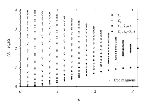
Figure 2: Excitation energy $(E\!-\!E_{F})/J$ versus wave number $k$ of all eigenstates in the invariant subspace with $r\!=\!2$ overturned spins for a system with $N\!=\!32$. Also shown are the corresponding data for free 2-magnon superpositions.

The class $C_{1}$ contains $N$ states for which one of the two Bethe quantum numbers is zero. This means that one of the magnons has zero wave number. Its effect is a slight rotation of the magnon vacuum, in which the other magnon is as free to propagate as in the original vacuum. There is no dynamical interaction. All states in this class are, effectively, 1-magnon states.

The class $C_{2}$ of states has nonzero Bethe quantum numbers $\lambda_{2}\!-\!\lambda_{1}\!\geq\!2$. There are $N(N\!-\!5)/2\!+\!3$ such pairs. All of them yield a solution with real $k_{1},k_{2}$, which makes them 2-magnon scattering states. A measure of the dynamical magnon interaction in Fig. 2 is the vertical displacement of any true scattering state $(\circ)$ from the nearest free-magnon pair (+). As $N$ increases, the energy correction diminishes for all class $C_{2}$ states and vanishes in the limit $N\!\to\!\infty$. The 2-magnon scattering states and the free 2-magnon states then form two-parameter continua with identical boundaries $E\!-\!E_{F}\!=\!2J[1\pm\cos(k/2)]$.

The class $C_{3}$ of states has nonzero Bethe quantum numbers which either are equal $\lambda_{2}\!=\!\lambda_{1}$, or differ by unity $\lambda_{2}\!=\!\lambda_{1}\!+\!1$. There exist $2N\!-\!3$ such pairs, but only $N\!-\!3$ pairs yield solutions of (16). For the class $C_{3}$ states, the effects of the dynamical magnon interaction are much more prominent, and the interaction energy does not disappear when $N\to\infty$. In Fig. 2, these states form a branch of 2-magnon bound states with dispersion $E\!-\!E_{F}\!=\!\frac{1}{2}J(1\!-\!\cos k)$ below the continuum of 2-magnon scattering states.

Figure 3: Weight distribution $|a(n_{1},n_{2})|$ versus distance $n_{2}\!-\!n_{1}$ of the two down spins of class $C_{3}$ states at $k\!=\!(2\pi/N)n,\;n\!=\!4,8,\ldots,N/2$ for $N\!=\!128$.

The bound state character of the class $C_{3}$ states manifests itself in the enhanced probability that the two flipped spins are on neighboring sites of the lattice. This property of the wave function is best captured in the weight distribution $|a(n_{1},n_{2})|$ of basis vectors with flipped spins at sites $n_{1}$ and $n_{2}$. In Fig. 3 we have plotted $|a(n_{1},n_{2})|$ versus $n_{2}-n_{1}$ for a sequence of class $C_{3}$ states between $k=0$ and $k=\pi$.[10] The distribution is peaked at $n_{2}-n_{1}=1$. Its width is controlled by the imaginary parts of $k_{1},k_{2}$ in (15). The smallest width is observed in the bound state at $k=\pi$. In this case, all coefficients with $n_{2}\neq n_{1}+1$ are zero, which implies that the two down spins are tightly bound together and have the largest binding energy.

The width of the distribution $|a(n_{1},n_{2})|$ increases as $k$ decreases, and the binding of the two down spins loosens. For finite $N$, the Bethe ansatz solutions switch from complex to real when the distribution has acquired a certain width. In scattering states the distribution $|a(n_{1},n_{2})|$ is always broad and tends to oscillate wildly. Some scattering states have a smooth distribution with a maximum for $n_{2}=n_{1}+N/2$, when the two down spins are farthest apart. The formation of bound states and scattering states of elementary excitations exist in many different contexts. But only in rare cases such as this one can they be investigated on the level of detail presented here.

4 Spinons Excited from Spin-Fluid State

Turning our attention to the Heisenberg antiferromagnet, we consider the Hamiltonian $H_{A}\!\equiv\!-H_{F}$ with $H_{F}$ defined in Eq. (12). All the eigenvectors remain the same, but the energy eigenvalues have the opposite sign. The magnon vacuum $|F\rangle$ now is at the top of the excitation spectrum. The ground state $|A\rangle$ of $H_{A}$ is located in the invariant subspace with $S_{T}^{z}=0$. This subspace also contains the two Néel states $|{\mathcal{N}}_{1}\rangle\equiv|\!\uparrow\downarrow\uparrow\cdots\downarrow\rangle,|{\mathcal{N}}_{2}\rangle\equiv|\!\downarrow\uparrow\downarrow\cdots\uparrow\rangle$, which are not eigenstates of $H_{A}$. In the framework of the Bethe ansatz, $|A\rangle$ can be obtained from $|F\rangle$ by exciting $r=N/2$ magnons with momenta $k_{i}$ and (negative) energies $-J(1-\cos k_{i})$. The Bethe quantum numbers for this state are $\{\lambda_{i}\}_{A}=\{1,3,5,\ldots,N-1\}$.

For reasons of computational convenience we rewrite the Bethe ansatz equations (16) in terms of the variables $z_{i}\equiv\cot(k_{i}/2)$:

$$N\arctan z_{i}=\pi I_{i}+\sum_{j\neq i}\arctan\left(\frac{z_{i}-z_{j}}{2}\right),\quad i=1,\ldots,r.$$ (18)

The associated Bethe quantum numbers $-N/2<I_{i}\leq N/2$ are integers for odd $r$ and half integers for even $r$. The relation between the sets $\{\lambda_{i}\}$ and $\{I_{i}\}$ depends on the configuration of the solution $\{z_{i}\}$ in the complex plane. Given the solution $\{z_{1},\ldots,z_{r}\}$ of Eqs. (18) for a state specified by $\{I_{1},\ldots,I_{r}\}$, its energy and wave number are

$$\frac{E-E_{F}}{J}=-\sum_{i=1}^{r}\frac{2}{1+z_{i}^{2}},\quad k=\pi r-\frac{2\pi}{N}\sum_{i=1}^{r}I_{i},$$ (19)

with $E_{F}=JN/4$. For states with real $\{z_{i}\}$, Eqs. (18) can be converted into a convergent iterative process:

$$z_{i}^{(n+1)}=\tan\biggl{(}\frac{\pi}{N}I_{i}+\frac{1}{N}\sum_{j\neq i}^{r}\arctan\bigl{[}\frac{z_{i}^{(n)}-z_{j}^{(n)}}{2}\bigr{]}\biggr{)}$$ (20)

with starting values $z_{i}^{(1)}=\pi I_{i}/N$. For the ground state $|A\rangle$ we have

$$\{I_{i}\}_{A}=\biggl{\{}-\frac{N}{4}+\frac{1}{2},~{}-\frac{N}{4}+\frac{3}{2},\ldots,\frac{N}{4}-\frac{1}{2}\biggr{\}}.$$ (21)

High-precision solutions $\{z_{i}\}$ can be obtained with little computational effort. The ground-state energy per site for $N\!=\!4096$, for example, reproduces the exact result $(E_{A}\!-\!E_{F})/JN\!=\!-\ln 2$ of the infinite chain to within 1 part in a million.[11] The distribution of magnon momenta in the ground state $|A\rangle$ is broad and peaked at $k_{i}=\pi$:

$$\rho_{0}(k_{i})=\left[8\sin^{2}\frac{k_{i}}{2}\cosh\left(\frac{\pi}{2}\cot\frac{k_{i}}{2}\right)\right]^{-1}.$$ (22)

This state, which has obviously a very complicated structure when described in terms of magnons, will now be configured as the physical vacuum of $H_{A}$ for a different kind of elementary particle called the spinon.[12]

A useful way to characterize the new physical vacuum is through the perfectly regular array (21) of Bethe quantum numbers as illustrated in the first row of Fig. 4.

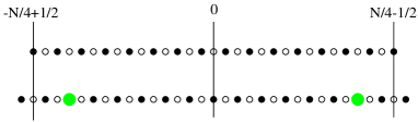
Figure 4: Configurations of Bethe quantum numbers $I_{i}$ for the $N\!=\!32$ ground state and for one representative of the 2-spinon (triplet) excitations with $S_{T}^{z}\!=\!S_{T}\!=\!1$. Each gap in one $I_{i}$-configuration (big circles) represents a spinon.

The spectrum of $H_{A}$ can then be generated systematically in terms of the fundamental excitations as characterized by elementary modifications of this vacuum array.

In the subspace with $S_{T}^{z}\!=\!1$, a two-parameter set of states is obtained by removing one magnon from the state $|A\rangle$. In doing so we eliminate one of the $N/2$ Bethe quantum numbers from the set in the first row of Fig. 4 and rearrange the remaining $I_{i}$ in all configurations over the expanded range $|I_{i}|\leq\frac{1}{4}N$. Changing $S_{T}^{z}$ by one means that the $I_{i}$ switch from half-integers to integers or vice versa. The number of distinct configurations with $I_{i+1}\!-\!I_{i}\geq 1$ is $N(N\!+\!2)/8$. A generic configuration consists of three clusters with two gaps between them as shown in the second row of Fig. 4. The position of the gaps between the $I_{i}$-clusters determine the momenta $\bar{k}_{1},\bar{k}_{2}$ of the two spinons, which, in turn, add up to the wave number of the two-spinon state relative to the wave number of the vacuum: $Q\equiv k\!-\!k_{A}\!=\!\bar{k}_{1}\!+\!\bar{k}_{2}$.

A plot of the 2-spinon energies $E-E_{A}$ versus wave number $k-k_{A}$ for $N=16$ as inferred via (19) from the solutions $\{z_{i}\}$ is shown in Fig. 5 ($\bullet$). The dots, which represent the corresponding data for $N=256$, produce a sort of density plot for the 2-spinon continuum which emerges in the limit $N\to\infty$. The exact lower and upper boundaries of the 2-spinon continuum are[13]

$$\omega_{L}(Q)=\frac{\pi}{2}J|\sin Q|,\quad\omega_{U}(Q)=\pi J|\sin\frac{Q}{2}|.$$ (23)

Like magnons, spinons carry a spin in addition to energy and momentum. Unlike magnons, which have spin 1, spinons are spin-$1/2$ particles. For even $N$, where all eigenstates have integer-valued $S_{T}^{z}$, spinons occur only in pairs. The spins $s_{1},s_{2}=\pm 1/2$ of the two spinons in a 2-spinon eigenstate of $H_{A}$ can be combined in four different ways to form a triplet state or a singlet state.

   

Figure 5: 2-spinon (triplet) excitations with $S_{T}^{z}=S_{T}=1$ for $N=16$ ($\bullet$) and $N=256$ (dots). Also shown are the 2-spinon (singlet) excitations with $S_{T}^{z}=S_{T}=0$ for $N=16$ ($\circ$).

We have already analyzed the spectrum of the 2-spinon triplet states with $s_{1}=s_{2}=+1/2$ $(S_{T}=1,\;S_{T}^{z}=+1)$. The 2-spinon triplets with $s_{1}=s_{2}=-1/2$ $(S_{T}=1,\;S_{T}^{z}=-1)$ are obtained from these states by a spin-flip transformation. One set of 2-spinon states with $s_{1}=-s_{2}$ are the triplets with $S_{T}^{z}\!=\!0$. They are obtained via Bethe ansatz by a simple modification of the $\{I_{i}\}$ configurations from the kind shown in the second row of Fig. 4 and yields an equal number of (real) solutions. Symmetry requires that all three triplet components $(S_{T}^{z}=0,\pm 1)$ are degenerate.

The 2-spinon singlet states $(S_{T}^{z}\!=\!S_{T}\!=\!0)$ are characterized by one pair of complex conjugate solutions $z_{1}\!=\!z_{2}^{\star}$ in addition to the real solutions $z_{3},\ldots,z_{N/2}$. Finding the $I_{i}$-configurations for a particular set of eigenstates with complex solutions and then solving the associated Bethe ansatz equations is, in general, delicate task.[11, 14] The 2-spinon singlets for $N\!=\!16$ and $0\!<\!Q\!\leq\!\pi$ are shown as open circles in Fig. 5. As $N$ grows large, the effect of the complex solutions $z_{1}\!=\!z_{2}^{\ast}$ on the energy relative to that of the real solutions $z_{3},\ldots,z_{N/2}$ diminishes. In the limit $N\to\infty$, the 2-spinon singlets also form a continuum with boundaries (23). Yet the effect of the complex solutions will remain strong for other quantities including selection rules and transition rates.

The 2-spinon triplets play an important role in the low-temperature spin dynamics of quasi-1D antiferromagnetic compounds such as $KCuF_{3}$, $Cu(C_{6}D_{5}COO)_{2}\cdot 3D_{2}O$, $Cs_{2}CuCl_{4}$, and $Cu(C_{4}H_{4}N_{2}(NO_{3})_{2})$. They are the elementary excitations of $H_{A}$ which can be directly probed via inelastic neutron scattering.[15] The 2-spinon singlets, in contrast, cannot be excited directly from $|A\rangle$ by neutrons because of selection rules. The singlet excitations are important nevertheless, but in a different context. Some quasi-1D antiferromagnetic compounds like $CuGeO_{3}$ are susceptible to a spin-Peierls transition, which involves a lattice distortion accompanied by an exchange dimerization.[16] The operator which probes the dimer fluctuations in the ground state of $H_{A}$ couples primarily to the 2-spinon singlets and not at all to the 2-spinon triplets.

5 Spinons Excited from Antiferromagnetic State

Although the computational application of the Bethe ansatz yields the exact wave functions of the 2-spinon states for very large systems with little effort, the very structure of the Bethe wave function makes it hard to use this knowledge for the calculation of the transition rates pertaining to any fluctuation operator of interest. Nevertheless, there exist ways to extract useful lineshape information from the Bethe wave function for specific situations.[17] Here we discuss an alternative approach, which exploits the higher symmetry of $H_{A}$ in the limit $N\to\infty$, described by the quantum group $U_{q}(sl_{2})$. For example, the asymptotic degeneracy of the 2-spinon triplets and singlets noted previously is attributable to this higher symmetry.

The algebraic analysis of a completely integrable spin chain employed for the purpose of calculating dynamic structure factors for specific fluctuation operators requires the execution of the following program:[18]

$\bullet~{}~{}$ Span the infinite-dimensional physically relevant Hilbert space in the form of a separable Fock space of multiple spinon excitations.
$\bullet~{}~{}$Generate the eigenvectors of the Hamiltonian in this Fock space by products of spinon creation operators (so-called vertex operators) from the ground state (physical vacuum).
$\bullet~{}~{}$Determine the spectral properties (energy, momentum) of the multiple-spinon states accessible from the ground state by the selected fluctuation operator.
$\bullet~{}~{}$Express the fluctuation operator of interest in terms of vertex operators.
$\bullet~{}~{}$Evaluate matrix elements of products of vertex operators as are needed for the selected fluctuation operator in the spinon eigenbasis.

In the following, we outline how this program was carried out for the calculation of the exact 2-spinon part of one dynamic structure factor for the 1D $s=\frac{1}{2}$ $XXZ$ model,

$$H_{XXZ}=-J\sum_{n=-\infty}^{\infty}(S_{n}^{x}S_{n+1}^{x}+S_{n}^{y}S_{n+1}^{y}+\Delta S_{n}^{z}S_{n+1}^{z}).$$ (24)

At $T=0$ $H_{XXZ}$ has a ferromagnetic phase for $\Delta\geq 1$, a critical phase (spin-fluid) for $-1\leq\Delta<1$, and an antiferromagnetic phase for $\Delta\!<\!-1$. The algebraic analysis operates in the massive phase stabilized by Néel LRO at $\Delta\!<\!-1$, but the isotropic limit $\Delta\!\to\!-1^{-}$, which is equivalent to $H_{A}$, can be performed meaningfully.

Each spinon in the $m$-spinon eigenstate $|\xi_{m},\epsilon_{m};\ldots;\xi_{1},\epsilon_{1}\rangle_{j}$ is characterized by a (complex) spectral parameter $\xi_{l}$ of unit length and a spin orientation $\epsilon_{l}\!=\!\pm 1$. The spectral properties then follow from the rules governing the application of the translation operator and the Hamiltonian:[18]

$$T|\xi_{m}\!,\!\epsilon_{m}\!;\!\ldots\!;\!\xi_{1}\!,\!\epsilon_{1}\rangle_{j} = \prod_{i=1}^{m}\frac{1}{\tau(\xi_{i})}|\xi_{m}\!,\!\epsilon_{m}\!;\!\ldots\!;\!\xi_{1}\!,\!\epsilon_{1}\rangle_{1\!-\!j},$$ (25)

$$H|\xi_{m}\!,\!\epsilon_{m}\!;\!\ldots\!;\!\xi_{1}\!,\!\epsilon_{1}\rangle_{j} = \sum_{i=1}^{m}e(\xi_{i})|\xi_{m}\!,\!\epsilon_{m}\!;\!\ldots\!;\!\xi_{1}\!,\!\epsilon_{1}\rangle_{j},$$ (26)

$$\tau(\xi) = e^{-ip(\xi)}=\xi^{-1}\frac{\theta_{q^{4}}(q\xi^{2})}{\theta_{q^{4}}(q\xi^{-2})},\quad e(\xi)=J\frac{1-q^{2}}{4q}\xi\frac{d}{d\xi}\log\tau(\xi),$$ (27)

$$\theta_{x}(y)\equiv(x;x)(y;x)(xy^{-1};x),\quad(y;x)\equiv\prod_{n=0}^{\infty}(1-yx^{n}).$$ (28)

Here $q$ is the deformation parameter of the quantum group $U_{q}(sl_{2})$. Its value is determined by the exchange anisotropy, $\Delta=(q+q^{-1})/2$. The twofold degenerate vacuum is represented by the vectors $|0\rangle_{0},|0\rangle_{1}$, which transform into each other via translation: $T|0\rangle_{j}=|0\rangle_{1-j}$. In the Ising limit $\Delta\to-\infty$, they become the pure Néel states $|\ldots\uparrow\downarrow\uparrow\downarrow\ldots\rangle,|\ldots\downarrow\uparrow\downarrow\uparrow\ldots\rangle$.

By eliminating $\xi$ from the relations (25) and (26) we obtain the spinon energy-momentum relation

$$e_{1}(p)=I\sqrt{1-k^{2}\cos^{2}p},\quad I\equiv\frac{JK}{\pi}\sinh\frac{\pi K^{\prime}}{K},$$ (29)

which is independent of the spin orientation. The elliptic integrals $K\equiv K(k),K^{\prime}\equiv K(k^{\prime})$ and their moduli $k,k^{\prime}\equiv\sqrt{1-k^{2}}$ depend on the anisotropy via $-q=\exp(-\pi K^{\prime}/K)$.

 

Figure 6: 2-spinon excitation spectrum for $k=0.99$ $(\Delta\simeq-2.305)$. It consists of two partly overlapping sheets $\mathcal{C}_{-}$ and $\mathcal{C}_{+}$. Sheet $\mathcal{C}_{+}$ lies between $\omega_{0}(Q)$ and $\omega_{-}(Q)$ in the range $Q_{\kappa}\leq Q\leq\pi-Q_{\kappa}$ and between $\omega_{+}(Q)$ and $\omega_{-}(Q)$ for $\pi-Q_{\kappa}\leq Q\leq\pi$. The interval $(0,\pi)$ represents one half of the extended Brillouin zone.

The of 2-spinon spectrum with energies $E(\xi_{1},\xi_{2})=e(\xi_{1})+e(\xi_{2})$ and momenta $P(\xi_{1},\xi_{2})=p(\xi_{1})+p(\xi_{2})$ is then a two-parameter set with fourfold spin degeneracy $\epsilon_{1},\epsilon_{2}=\pm 1$.[19] In the isotropic limit, they are the 2-spinon triplets and singlets discussed in Sec. 4. In a finite system, the singlet-triplet degeneracy is removed (see Fig. 5). Exchange anisotropy splits up the triplet levels as well.

In the $(Q,\omega)$ plane, each set of 2-spinon excitations forms a continuum (see Fig. 6) of two sheets $\mathcal{C}_{\pm}$ with boundaries

$$\omega_{0}(Q)=\frac{2I}{1+\kappa}\sin Q,\quad\omega_{\pm}(Q)=\frac{2I}{1+\kappa}\sqrt{1+\kappa^{2}\pm 2\kappa\cos Q},$$ (30)

where $\kappa\equiv\cos Q_{\kappa}=(1-k^{\prime})/(1+k^{\prime})$ is a convenient anisotropy parameter. The evaluation of the dynamic structure factor of any fluctuation operator $F_{Q}^{A}$, Eq. (9), requires that we know exact matrix elements ${}_{j}\langle 0|A_{l}|\xi_{m},\epsilon_{m},\ldots,\xi_{1},\epsilon_{1}\rangle_{j^{\prime}}$ for the associated local operators. In principle, they can be calculated exactly if we are able to express $A_{l}$ in terms of vertex operators. In practice, the exact results available thus far are limited to the dynamic spin structure factors

$$S_{\mu\mu}(Q,\omega)=\sum_{n=-\infty}^{+\infty}\int_{-\infty}^{\infty}dt\;e^{i(\omega t+Qn)}\langle S_{n}^{\mu}(t)S_{0}^{\mu}\rangle,\quad\mu=x,z.$$ (31)

In the $m$-spinon expansion $S_{zz}(Q,\omega)\!=\!S_{zz}^{(0)}(Q,\omega)\!+\!S_{zz}^{(2)}(Q,\omega)+\ldots$ we know the matrix elements that determine the leading term,[18]

$$2{{}_{j}}\langle 0|S_{n}^{z}|0\rangle_{j}=\frac{(q^{2};q^{2})^{2}}{(-q^{2};q^{2})^{2}}(-1)^{n+j}=\frac{2\pi}{K}\sqrt{k^{\prime}}=2\bar{m}_{z},$$ (32)

yielding $S^{(0)}_{zz}(Q,\omega)\!=\!4\pi^{2}\delta(\omega)\delta(Q-\pi)\bar{m}_{z}^{2},$ where $\bar{m}_{z}$ is the staggered magnetization.[20] No exact transition rates have been evaluated for the 2-spinon part $S_{zz}^{(2)}(Q,\omega)$ or any higher order term in the $m$-spinon expansion.

The corresponding $m$-spinon expansion of $S_{xx}(Q,\omega)$ starts with $m\!=\!2$, because the operator $S_{n}^{x}$ does not connect the vacuum sector with itself. All non-vanishing matrix elements which are needed for $S_{xx}^{(2)}(Q,\omega)$ can be expressed, as it turns out, by a single function $X^{j}(\xi_{2},\xi_{1})\equiv{{}_{j}\langle}0|\sigma_{0}^{+}|\xi_{2},-;\xi_{1},-\rangle_{j}$, which was determined by Jimbo and Miwa:[18]

$$X^{j}(\xi_{2},\xi_{1})=\varrho^{2}\frac{(q^{4};q^{4})^{2}}{(q^{2};q^{2})^{3}}\frac{(-q\xi_{1}\xi_{2})^{1-j}\xi_{1}\gamma(\xi_{1}^{2}/\xi_{2}^{2})\theta_{q^{8}}(-\xi_{1}^{-2}\xi_{2}^{-2}q^{4j})}{\theta_{q^{4}}(-\xi_{1}^{-2}q^{3})\theta_{q^{4}}(-\xi_{2}^{-2}q^{3})},$$ (33)

where $(x;y;z)\equiv\prod_{n,m=0}^{\infty}\left(1-xy^{n}z^{m}\right)$ and

$$\gamma(\xi) \equiv \frac{(q^{4}\xi;q^{4};q^{4})(\xi^{-1};q^{4};q^{4})}{(q^{6}\xi;q^{4};q^{4})(q^{2}\xi^{-1};q^{4};q^{4})},\quad\varrho\equiv(q^{2};q^{2})^{2}\frac{(q^{4};q^{4};q^{4})}{(q^{6};q^{4};q^{4})}.$$ (34)

These ingredients yield the following expression to be evaluated:[21]

$$S^{(2)}_{xx}(Q,\omega) = \frac{1}{4}\oint\frac{d\xi_{1}}{2i\xi_{1}}\frac{d\xi_{2}}{2i\xi_{2}}\delta[\omega-E(\xi_{1},\xi_{2})]$$ (35)

$$\times\{\delta[Q+P(\xi_{1},\xi_{2})]|X^{0}(\xi_{2},\xi_{1})+X^{1}(\xi_{2},\xi_{1})|^{2}$$

$$+\delta[Q-\pi+P(\xi_{1},\xi_{2})]|X^{0}(\xi_{2},\xi_{1})-X^{1}(\xi_{2},\xi_{1})|^{2}\}.$$

A compact rendition of the exact result reads[21]

$$S_{xx}^{(2)}(Q,\omega)=\frac{\omega_{0}}{8I\omega}\left[1\!+\!\sqrt{\frac{\omega^{2}\!-\!\kappa^{2}\omega^{2}_{0}}{\omega^{2}\!-\!\omega^{2}_{0}}}\right]\sum_{c=\pm}\frac{\vartheta_{A}^{2}(\beta_{-}^{c})}{\vartheta_{d}^{2}(\beta_{-}^{c})}\frac{|\tan(Q/2)|^{-c}}{W_{c}},$$ (36)

where

$$W_{\pm}=\sqrt{\frac{\omega_{0}^{4}}{\omega^{4}}\kappa^{2}-\left(\frac{T}{\omega^{2}}\pm\cos Q\right)^{2}},\quad T=\sqrt{\omega^{2}-\kappa^{2}\omega_{0}^{2}}\sqrt{\omega^{2}-\omega_{0}^{2}},$$ (37)

$$\beta_{-}^{c}(Q,\omega)=\frac{1+\kappa}{2}F\left[\arcsin\left(\frac{2I\omega W_{c}}{\kappa(1+\kappa)\omega_{0}^{2}}\right),\kappa\right],$$ (38)

$$\vartheta_{A}^{2}(\beta)=\!\exp\left(\!-\sum_{l=1}^{\infty}\frac{e^{\gamma l}}{l}\frac{\cosh(2\gamma l)\cos(t\gamma l)-1}{\sinh(2l\gamma)\cosh(\gamma l)}\right),$$ (39)

$\gamma=\pi K^{\prime}/K$, $t\equiv 2\beta/K^{\prime}$, and $\vartheta_{d}(x)$ is a Neville theta function. This function is plotted in Fig. 7 for $(Q,\omega)\in\mathcal{C_{+}}$. $S_{xx}^{(2)}(Q,\omega)$ has a square-root divergence at the portion $\omega_{0}(Q)$ of the spectral threshold. Along the portion $\omega_{+}(Q)$ of the lower boundary and along the entire upper boundary of $\mathcal{C}_{+}$, $S_{xx}^{(2)}(Q,\omega)$ has a square-root cusp. The line shapes for $(Q,\omega)\in\mathcal{C_{-}}$ are inferred from the symmetry property $S_{xx}^{(2)}(\pi-Q,\omega)=S_{xx}^{(2)}(Q,\omega)$.

Figure 7: 2-spinon dynamic structure factor $S_{xx}^{(2)}(Q,\omega)$ for $(Q,\omega)\in\mathcal{C_{+}}$ as a function of frequency for wave numbers $Q_{\kappa}\leq Q\leq\pi$ and anisotropy parameter $k=0.7435$ ($\Delta\simeq-10$), $k=0.8279$ ($\Delta\simeq-7$), $k=0.8976$ ($\Delta\simeq-5$), and $k=0.99$ ($\Delta\simeq-2.305$).

The isotropic limit $\Delta\to-1^{-}$ is delicate because of its singular nature. As the LRO in the spinon vacuum vanishes, the size of the Brillouin zone changes from $(-\pi/2,+\pi/2)$ to $(-\pi,+\pi)$. A practical consequence of this phase transition is that we switch our perspective from considering both sheets $\mathcal{C}_{\pm}$ of 2-spinon excitations over the range $(-\pi/2,+\pi/2)$ to considering only the sheet $\mathcal{C}_{+}$, now with boundaries (23), over the extended range $(-\pi,+\pi)$. With these subtleties taken into account, Eq. (36) reduces to[22]

$$S_{xx}^{(2)}(Q,\omega)=\frac{1}{2}[\omega_{U}^{2}(Q)-\omega^{2}]^{-1/2}e^{-I(t)},$$ (40)

$$I(t)=\int_{0}^{\infty}dx\frac{\cosh 2x\cos xt-1}{x\sinh 2x\cosh x}e^{x},\quad\frac{\pi t}{4}={\rm cosh}^{-1}\sqrt{\frac{\omega_{U}^{2}(Q)-\omega_{L}^{2}(Q)}{\omega^{2}-\omega_{L}^{2}(Q)}}.$$ (41)

This function, which is plotted in Fig. 8, has a square-root cusp at $\omega_{U}(Q)$ and a square-root divergence with logarithmic corrections at $\omega_{L}(Q)$.

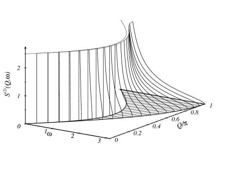
Figure 8: Exact 2-spinon dynamic spin structure factor. The expression is nonzero only in the shaded region of the $(Q,\omega)$-plane bounded by $\omega_{L}(Q)$ and $\omega_{U}(Q)$.

6 Solitons Excited from Néel State

Near the Ising limit ($\Delta\to-\infty$), the exact result (36) can be expanded in powers of the anisotropy parameter $\kappa$. To leading order, we obtain

$$S_{xx}^{(2)}(Q,\omega)\to\frac{1}{2\cos^{2}Q}\sqrt{\cos^{2}Q-\left(\frac{\Omega}{\kappa}\right)^{2}\Theta(\kappa|\cos Q|-|\Omega|)}$$ (42)

with $\Omega\equiv\omega/2I-1$, which is identical (in that order) to the result obtained by Ishimura and Shiba[23] from a first-order perturbation calculation about the Ising limit. In their calculation, the two vacuum states are approximated by the pure Néel states (see Fig. 9). The spinons are kink solitons (domain walls),[24] which produce two adjacent up or down spins in an otherwise unperturbed Néel configuration. The only states which contribute to $S_{xx}(Q,\omega)$ in leading order of the perturbation calculation are states which contain two solitons with equal spin orientation. The states with solitons of opposite spin orientation dominate the spectrum of $S_{zz}(Q,\omega)$ except for the central peak at $\omega=0,\;Q=\pi$, which involves a transition between the two vacuum states.

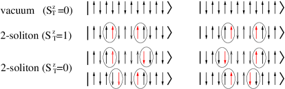
Figure 9: Local basis states from which translationally invariant Néel states and 2-soliton states are constructed. The latter are limiting cases of the 2-spinon states discussed in Sec. 5.

The 2-soliton spectrum with boundaries $|\Omega|\leq\kappa\cos Q$, is akin to the generic 2-spinon spectrum shown in Fig. 6, but it does not capture any of the features that characterize the regime $Q_{\kappa}\leq Q\leq\pi-Q_{\kappa}$ around the Brillouin zone boundary. The limitations of the perturbation results are much less severe near the center of the Brillouin zone. This illustrated in Fig. 10, which compares the line shapes of Eq. (36) and (42) at $Q=\pi$. Here a fairly strong departure from the Ising limit is required before a significant difference between the two results is produced.

Figure 10: Line shapes of $S_{xx}^{(2)}(Q,\omega)$ at the zone center $Q=\pi$ as established by the exact result (36) (solid line) and predicted by the first order perturbation result (42) (dashed line).

Two intensively studied physical realizations of $H_{XXZ}$ at $\Delta<-1$ are $\rm CsCoCl_{3}$ and $\rm CsCoBr_{3}$. Spectroscopic data which probe both the quantum and thermal fluctuations of those materials are available from several neutron scattering experiments.[25]

References

- [1] B. J. Berne and G. D. Harp, Adv. Chem. Phys. XVII, 63 (1970);
- [2] U. Schollwöck, T. Jolicoeur, and T. Garel, Phys. Rev. B 53, 3304 (1996).
- [3] L. A. Takhtajan, Phys. Lett. A 87, 479 (1982); H. M. Babujian, Nucl. Phys. B 215, 317 (1983); G. V. Uimin, JEPT Lett. 12, 225 (1970); C. K. Lai, J. Math. Phys. 15, 1675 (1974); B. Sutherland, Phys. Rev. B 12, 3795 (1975);
- [4] V. S. Viswanath and G. Müller, The Recursion Method, LNP m23 (Springer-Verlag, Heidelberg, 1994); A. Fledderjohann, M. Karbach, K.-H. Mütter, and P. Wielath, J. Phys.: Condens. Matter 7, 8993 (1995).
- [5] A. Schmitt et al., Phys. Rev. B 58, 5498 (1998).
- [6] I. Affleck, T. Kennedy, E. Lieb, and H. Tasaki, Phys. Rev. Lett. 59, 799 (1987); D. P. Arovas, A. Auerbach, and F. D. M. Haldane, Phys. Rev. Lett. 60, 531 (1988);
- [7] S. Ma et al., Phys. Rev. Lett. 69, 3571 (1992).; A. Zheludev et al., Phys. Rev. B 53, 15004 (1996).
- [8] F. J. Dyson, Phys. Rev. 102, 1217 (1956).
- [9] H. Bethe, Z. Phys. 71, 205 (1931).
- [10] M. Karbach and G. Müller, Comp. in Phys. 11, 36 (1997).
- [11] M. Karbach, K. Hu, and G. Müller, Comp. in Phys. 12, 565 (1998).
- [12] L. D. Faddeev and L. A. Takhtajan, Phys. Lett. A85, 375 (1981).
- [13] J. des Cloizeaux and J. J. Pearson, Phys. Rev. 128, 2131 (1962); T. Yamada, Prog. Theor. Phys. 41, 880 (1969).
- [14] F. Woynarovich, J. Phys. C: Solid St. Phys. 15, 6397 (1982).
- [15] S. E. Nagler et al., Phys. Rev. B 44, 12361 (1991); D. A. Tennant, T.G. Perring, R. A. Cowley, and S. E. Nagler, Phys. Rev. Lett. 70, 4003 (1993); D. A. Tennant, R. A. Cowley, S. E. Nagler, and A. M. Tsvelik, Phys. Rev. B 52, 13368 (1995); D. C. Dender et al., Phys. Rev. B 53, 2583 (1996); R. Coldea et al., Phys. Rev. Lett. 79, 151 (1997); P. R. Hammar et al., Phys. Rev. B 59, 1008 (1999).
- [16] M. Arai et al., Phys. Rev. Lett. 77, 3649 (1996); K. Fabricius et al., Phys. Rev. B 57, 1102 (1998).
- [17] M. Karbach, D. Biegel, K. Hu, and G. Müller (unpublished)
- [18] M. Jimbo and T. Miwa, Algebraic Analysis of Solvable Lattice Models, CBMS (American Mathematical Society, Providence, 1995).
- [19] J. D. Johnson and B. M. McCoy, Phys. Rev. A 6, 1613 (1972).
- [20] R. J. Baxter, J. Stat. Phys. 9, 145 (1973).
- [21] A. H. Bougourzi, M. Karbach, and G. Müller, Phys. Rev. B 57, 11429 (1998).
- [22] M. Karbach et al., Phys. Rev. B 55, 12510 (1997).
- [23] N. Ishimura and H. Shiba, Prog. Theor. Phys. 63, 743 (1980).
- [24] J. Villain, Physica B 79, 1 (1975).
- [25] H. Yoshizawa, K. Hirakawa, S. K. Satija, and G. Shirane, Phys. Rev. B 23, 2298 (1981); S. E. Nagler, W. J. L. Buyers, R. L. Armstrong, and B. Briat, Phys. Rev. B 27, 1784 (1983); J. P. Goff, D. A. Tennant, and S. E. Nagler, Phys. Rev. B 52, 15992 (1995); S. E. Nagler, W. J. L. Buyers, R. L. Armstrong, and B. Briat, Phys. Rev. B 27, 1784 (1983); J. P. Boucher et al., Phys. Rev. B 31, 3015 (1985).