[

Composite fermions close to the one-half filling of the lowest Landau level revisited

Abstract

By strictly adhering to the microscopic theory of composite fermions (CFs) for the Landau-level filling fractions $\nu_{\rm e}=p/(2p+1)$, we reproduce, with remarkable accuracy, the surface-acoustic-wave (SAW)-based experimental results by Willett and co-workers concerning two-dimensional electron systems with $\nu_{\rm e}$ close to $1/2$. Our results imply that the electron band mass $m_{b}$, as distinct from the CF mass $m_{\star}$, must undergo a substantial increase under the conditions corresponding to $\nu_{\rm e}\approx 1/2$. We further establish that a finite mean-free path $\ell_{0}$ is essential for the observed linearity of the longitudinal conductivity $\sigma_{xx}(q)$ as deduced from the SAW velocity shifts.

]

The fractional quantum Hall effect (FQHE) owes its existence to the electron-electron (e-e) interaction. The fermionic Chern-Simons field theory in $2+1$ dimensions unifies the FQHE with the integer QHE (IQHE) whose existence does not depend on e-e interaction [1, 2, 3]. This is effected through the binding, brought about by the mediation of the Chern-Simons action, of $2n$, $n=1,2,\dots$, magnetic flux quanta to electrons, whereby the composite particles, that is CFs [4], are exposed to an effective magnetic flux density $\Delta B$ whose corresponding IQH state determines the FQH state for the electrons; the FQH state associated with $\nu_{\rm e}=p/(2np+1)$ is the IQH state of CFs in which $p$ lowest Landau levels (LLs) are fully occupied. The sequence $\nu_{\rm e}=p/(2np+1)$ and its particle-hole conjugate $\nu_{\rm e}^{\prime}{:=}1-p/(2np+1)$ approach $\nu_{\rm e}=1/(2n)$ for $p\to\infty$. In this work we deal with the case where $n=1$ and states whose $\nu_{\rm e}$ are close to $1/2$. With $\Delta B\equiv hn_{e}/(ep)$, where $-e<0$ stands for the charge of an electron and $n_{e}$ the planar number density of electrons, these states thus correspond to small $\Delta B$. The state corresponding to $\nu_{\rm e}=1/2$ was proposed by Halperin, Lee and Read [3] to be a compressible state of degenerate fermions which, in the case of full polarisation of the electron spins, is characterised by a cylindrical Fermi surface of radius $k_{F}^{\sc cf}=\sqrt{4\pi n_{e}}$. This has been borne out by several experiments [5, 6, 7, 8, 9].

In this work we particularly concentrate on a series of experimental results by Willett and co-workers [5, 6, 10], concerning 2DESs with $\nu_{\rm e}$ at and close to $1/2$ and establish that these can be remarkably accurately reproduced within the framework of the microscopic Chern-Simons field theory. To achieve this, it turns out to be essential that the band-electron mass $m_{b}$ be by one order of magnitude larger than the customarily-assumed value: for GaAs heterostructures, in which the 2DESs under consideration were realised, $m_{b}$ is customarily taken to be $0.067\times m_{e}$, where $m_{e}$ is the electron mass in vacuum. In what follows, we use the notation $m_{b}^{0}=0.067\times m_{e}$ and denote the electron band mass, as required for reproducing the indicated experimental results, by $m_{b}$. Since quantum fluctuations, with respect to the mean-field approximation for CFs give rise to mass renormalisation [3], we reserve $m_{\star}$ to denote the renormalised CF mass. Our numerical results imply $m_{b}{\mathstrut{}_{\displaystyle{\sim}}^{\displaystyle>}}16\times m_{b}^{0}$ and $m_{\star}\approx 0.5\times m_{b}{\mathstrut{}_{\displaystyle{\sim}}^{\displaystyle>}}8\times m_{b}^{0}\approx 0.54\times m_{e}$. This value is in good accord with the CF mass as deduced both from the values of the energy gaps $\Delta_{\nu_{e}}$ separating the CF LLs (determined from the activated temperature dependence of the longitudinal resistivities, $\varrho_{xx}$, centred around $\nu_{e}$’s close to $1/2$) [11, 12, 13, 10] and the amplitude of the oscillations in $\varrho_{xx}$, for varying $\Delta B$, viewing these as the Shubnikov-de Haas oscillations corresponding to CFs [14, 15, 16, 13, 10]. For completeness, according to Park and Jain [17], the scale of the low-energy excitations of a 2DES may be determined by either the ‘activation mass’ $m_{a}$ or the ‘polarisation mass’ $m_{p}$, the latter being often the case for $\nu_{\rm e}>1$. For $\nu_{\rm e}=1/2$ ($n_{e}=1.26\times 10^{11}$ cm^-2) Kukushkin, et al. [18] have reported a CF mass equal to $2.27\times m_{e}$ which the authors suggest to be the $m_{p}$ of CFs. In view of the fact that the experiments in Ref. [18] are based on optical excitations, involving $q\approx 0$, we suggest the possibility that the mass measured by these authors may be not $m_{p}$, but $m_{b}$, consistent with the requirement of a Kohn’s theorem [19] (note the aspect $q\approx 0$).

In the experiments by Willett, et al. [5, 6, 10], the relative change $\Delta v_{s}/v_{s}$ in the velocity $v_{s}$ of SAWs as well as the damping $\kappa$ in their amplitudes, while propagating on the surface of samples at distance $d$ from the 2DES, were measured; here the change $\Delta v_{s}$ is relative to the $v_{s}$ corresponding to the case where the conductivity of the 2DES is infinitely large (see further on). Theoretically, $\Delta v_{s}/v_{s}$ is determined by the ‘on-the-mass-shell’ value of the longitudinal conductivity $\sigma_{xx}(q,\omega)$ of the 2DES as follows

$$\frac{\Delta v_{s}}{v_{s}}=\frac{\alpha^{2}/2}{1+[\sigma_{xx}(q)/\sigma_{m}]^{2}},$$ (1)

where $\sigma_{xx}(q)\equiv\sigma_{xx}(q,\omega=v_{s}q)$, $\sigma_{m}$ is a constant to be specified below, and [20] $\alpha^{2}/2=$ $(e_{14}^{2}\tilde{\epsilon}_{r}/\{H\epsilon_{0}\epsilon_{r}^{2}\})$ $|F(qd)|^{2}$; here $e_{14}\approx 0.145$ Cm^-2 is the piezoelectric constant for Al_xGa_1-xAs, $\tilde{\epsilon}_{r}=\epsilon_{r}\big{(}1+\{(\epsilon_{r}-1)/(\epsilon_{r}+1)\}\exp(-2qd)\big{)}^{-1}$ (c.f. Eq. (A4) in Ref. [20]), $H\approx 28.8\times 10^{10}$ Nm^-2, $\epsilon_{0}=8.854\dots\times 10^{-12}$ Fm^-1 denotes the vacuum permittivity, $\epsilon_{r}$ is the relative dielectric constant of the bulk of the host material which we take to be equal to $12.4$, and $F(x){:=}A_{1}\exp(-ax)\sin(bx+c)+A_{2}\exp(-x)$ (c.f. Eq. (51) in Ref. [20]), where $A_{1}\approx 3.18$, $a\approx 0.501$, $b\approx 0.472$, $c\approx 2.41$ and $A_{2}\approx-3.10$; further,

$$\sigma_{m}{:=}\left.\frac{\omega e^{2}}{q^{2}v(q)}\right|_{\omega=v_{s}q}\equiv 2\epsilon_{0}\tilde{\epsilon}_{r}v_{s},$$ (2)

where in the second expression on the right-hand side we have replaced the e-e interaction function $v(q)$ by the Coulomb function $v(q)=e^{2}/(2\epsilon_{0}\tilde{\epsilon}_{r}q)$; we have further made use of the dispersion of acoustic phonons and employed $\omega=v_{s}q$, where $v_{s}$ stands for the sound velocity which in GaAs amounts to $3010$ ms^-1.

Our calculations are based on [3] (see also Eq. (208) in Ref. [21]) $\Delta v_{s}/v_{s}+i\kappa/q=(\alpha^{2}/2)\big{(}\gamma-v(q)K_{00}(q,\omega=v_{s}q)\big{)}$, where $-K_{00}(q,\omega)$ describes the change in $n_{e}$ to linear order in the external potential [1, 2, 3, 22]; the minus sign here has its origin in our convention with regard to the sign of $e$. In the literature, the constant $\gamma$ is invariably identified with unity, this on account of the fact that $\Delta v_{s}$ is the deviation of the measured $v_{s}$ with respect to the $v_{s}$ pertaining to the case where $\sigma_{xx}(q)\to\infty$. We maintain $\gamma$ in our considerations, following the fact that, experimentally, the reference $v_{s}$ does not correspond to an infinitely large $\sigma_{xx}(q)$ (owing to impurities, and $q\not\approx 0$).

In the present work we employ the ‘modified random phase approximation’ (MRPA) for $K_{00}(q,\omega)$ due to Simon and Halperin [22] which takes account of the renormalisation of the mass of CFs and which approaches the RPA for $K_{00}(q,\omega)$ as $q\to 0$, the latter coinciding to leading order (proportional to $q^{2}$) with the exact $K_{00}(q,\omega)$ for $q\to 0$ and any $\omega$ at which both $K_{00}^{\sc rpa}(q,\omega)$ and $K_{00}(q,\omega)$ are bounded, which is the case for $|\omega|<\Delta\omega_{c}{:=}e\Delta B/m_{b}$ (see in particular Eq. (5.6) in Ref. [23]). The $K_{00}^{\sc mrpa}$ has thus the property that it conforms with the requirement of a Kohn’s theorem [19] according to which $K_{00}(q\to 0,\omega)$ must be determined by $m_{b}$ rather than $m_{\star}$. For the explicit expression concerning $K_{00}^{\sc mrpa}(q,\omega)$ corresponding to $\nu_{\rm e}=p/(2np+1)$ in terms of elementary functions, we refer the reader to Ref. [22] (we have presented and employed $K_{00}^{\sc mrpa}(q,\omega=0)$ in Ref. [24]). We mention that for the purpose of calculating $K_{00}^{\sc mrpa}(q,\omega)$, which depends on $p$ and $n$, for a continuous range of $\Delta B$ around zero, we first determine $\nu_{\rm e}$ from $\nu_{\rm e}=hn_{e}/(eB)$, with $B$ the total applied magnetic flux density, and subsequently obtain the required $p$ from $p=[\nu_{\rm e}/(1-2\nu_{\rm e})]$ if $\nu_{\rm e}<1/2$, and $p=[(1-\nu_{e})/(1-2(1-\nu_{\rm e}))]$ if $\nu_{\rm e}>1/2$, where $[x]$ denotes the greatest integer less than or equal to $x$. The $\nu_{\rm e}$ corresponding to the thus-obtained $p$ remains constant for certain ranges of values of $B$, which causes artificial stepwise-constant behaviour in the functions of $\Delta B$ that depend on $K_{00}^{\sc mrpa}(q,\omega)$.

We model the effects of the impurity scattering through substituting $\omega+i/\tau_{0}$ for $\omega$ in $K_{00}^{\sc mrpa}(q,\omega)$. Here $\tau_{0}$ stands for the scattering time which is related to the mean-free path $\ell_{0}=v_{F}\tau_{0}$, where $v_{F}$ stands for the Fermi velocity. In general, the substitution $\omega\rightharpoonup\omega+i/\tau_{0}$ amounts to solving the Boltzmann equation within the framework of the relaxation-time approximation, neglecting the so-called current-conservation correction which has been found to have no significant consequences in contexts similar to that of our present considerations (see Sec. 4.1.4 in Ref. [21]). With (from here onwards we suppress ‘mrpa’) $K^{\prime}_{00}(q,\omega+i/\tau_{0})\equiv{\rm Re}\big{\{}K_{00}(q,\omega+i/\tau_{0})\big{\}}$ and $\gamma^{\prime}{:=}{\rm Re}\{\gamma\}$, from the above-presented expression for $\Delta v_{s}/v_{s}+i\kappa/q$ we obtain

$$\frac{\Delta v_{s}}{v_{s}}=\frac{\alpha^{2}}{2}\big{(}\gamma^{\prime}-v(q)K_{00}^{\prime}(q,v_{s}q+i/\tau_{0})\big{)}.$$ (3)

We eliminate $\gamma^{\prime}$, whose value has no influence on the form of $\Delta v_{s}/v_{s}$, by requiring that $\Delta v_{s}/v_{s}$, as a function of $\Delta B$, coincide with the experimental $\Delta v_{s}/v_{s}$ for $\Delta B\approx 0$.

In Fig. 1 we present $\Delta v_{s}/v_{s}$ as a function of $\Delta B$ for the cases where $n_{e}=6.92\times 10^{10}$ cm^-2, $f{:=}\omega/(2\pi)=8.5$ GHz (left panel), to be compared with Fig. 4 in Ref. [6], and $n_{e}=1.6\times 10^{11}$ cm^-2, $f=10.7$ GHz (right panel), to be compared with Fig. 1 in Ref. [10]. The excellent agreement between the theoretical results corresponding to an enhanced $m_{b}$ (with respect to $m_{b}^{0}$) and experimental results, in particular when these are compared with those obtained within the same theoretical framework in which $m_{\star}$ retains the same enhanced value as compared with $m_{b}^{0}$ but $m_{b}=m_{b}^{0}$ (curves (c)), strongly support the viewpoint that under the conditions where $\nu_{\rm e}\approx 1/2$, the bare band mass $m_{b}^{0}$ should be enhanced. This observation is compatible with the experimental finding with regard to the stronger than the theoretically-predicted divergence [3] of the CF mass for $\nu_{\rm e}\to 1/2$ [12, 13, 15, 16]. In this connection we should emphasise that the closer one approaches $\nu_{\rm e}=1/2$, the less sensitive $\Delta v_{s}/v_{s}$ becomes with respect to the further increase of $m_{\star}$ (or $m_{b}$ for that matter); our choices $m_{b}=16\times m_{b}^{0}$ and $m_{\star}=0.5\times m_{b}$ are based on the consideration that the experimental features corresponding to $\Delta B$ in the range $\sim 0.1-1$ T be reproduced. The results in Fig. 1 obtained through employing the semi-classical $\sigma_{\mu\nu}$, due to Cohen, Harrison and Harrison (CHH) [25] (see also Appendix B in Ref. [3] as well as Eqs. (2) and (3) in Ref. [6]), bring out the inadequacy of the semi-classical approach; curves marked by (d) unequivocally demonstrate the shortcoming of strictly adhering to the viewpoint that CFs behaved like non-interacting electrons exposed to a reduced magnetic field — curves marked by (b), which are similarly based on the CHH $\sigma_{\mu\nu}$, owe their resemblance to the experimental results to the fact that in their calculation explicit account has been taken of the conditions which are specific to the regime corresponding to $\nu_{\rm e}\approx 1/2$. With reference to our earlier work [24], it is appropriate to compare curve (a) in the right panel of Fig. 1 with the curves in Fig. 1 of the work by Mirlin and Wölfle [26] and compare both with the experimental trace in Fig. 1 of Ref. [10]. One observes that our present result, in contrast with those in Ref. [26], precisely reproduces almost all features of the experimental trace, such as the values of $\Delta v_{s}/v_{s}$ at $\Delta B\approx 0,0.38,0.54,1.0$ T.

From Eqs. (1) and (3) we obtain

$$\frac{\sigma_{xx}(q)}{\sigma_{m}}=\Big{(}\big{(}\gamma^{\prime}-v(q)K^{\prime}_{00}(q,v_{s}q+i/\tau_{0})\big{)}^{-1}-1\Big{)}^{1/2},$$ (4)

according to which $\sigma_{xx}(q)$ interestingly does not explicitly depend upon $\alpha^{2}/2$. Unless we set $\gamma^{\prime}=1$, we eliminate $\gamma^{\prime}$ in Eq. (4) by requiring that for given values of $\sigma_{m}$ and $q$, $\sigma_{xx}(q)$ according to Eq. (4) yield the corresponding experimental SAW velocity shift.

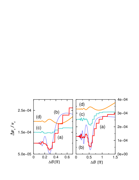
FIG. 1.: (colour) The relative shift of the SAW velocity. (a) and (c) are obtained from Eq. (3), while (b) and (d) are based on Eq. (1) in which the semi-classical result for $\sigma_{\mu\nu}$, due to CHH [25], has been employed: for (d), $\sigma_{xx}(q)$ has been directly used, whereas for (b) $\sigma_{xx}(q)$ has been obtained from $\sigma_{yy}(q)$ according to $\sigma_{xx}(q)\approx(\nu_{e}e^{2}/h)^{2}|_{\nu_{e}=1/2}/\sigma_{yy}(q)$ — this expression takes explicit account of the fact that for $\nu_{e}\approx 1/2$, $\varrho_{xx}\varrho_{yy}\ll\varrho_{xy}^{2}$ and $\varrho_{yy}\approx 1/\sigma_{yy}$; in both cases we have scaled $\sigma_{xx}/\sigma_{m}$ by a constant such that for $\nu_{\rm e}=1/2$ the corresponding $\Delta v_{s}/v_{s}$ coincide with the experimental value (for clarity we have offset (d) by $10^{-4}$ in the left panel and by $2\times 10^{-4}$ in the right). The equality of (a) and (c) (we have offset (c) by $5\times 10^{-5}$ in the left panel and by $1.75\times 10^{-4}$ in the right) with the associated experimental results at $\nu=1/2$ has been enforced through appropriate choices for $\gamma^{\prime}$ ($\approx 1.1$). Left panel: $n_{e}=6.92\times 10^{10}$ cm^-2, $\ell_{0}=0.4$ $\mu$m, $d=10$ nm, $f=8.5$ GHz. Right panel: $n_{e}=1.6\times 10^{11}$ cm^-2, $\ell_{0}=0.6$ $\mu$m (corresponding to $\tau_{0}=19.6$ ps), $d=100$ nm, $f=10.7$ GHz. Both panels: (a), $m_{b}=16\times m_{b}^{0}$, $m_{\star}=0.5\times m_{b}$; (c), $m_{b}=m_{b}^{0}$, $m_{\star}=8\times m_{b}$. For the origin of the step-like behaviour in curves (a) and (c) see the main text.

In Fig. 2 we present our theoretical $\sigma_{xx}(q)$ in comparison with its SAW-derived experimental $\sigma_{xx}(q)$ by Willett, et al. [5] (see the middle panel of Fig. 2 herein). The details in Fig. 2 again support our above finding with regard to $m_{b}$ and $m_{\star}$, that a mere enhancement of $m_{\star}$ with respect to $m_{b}^{0}$ is not sufficient (see inset [B]). We also observe that a finite $\ell_{0}$ is most crucial to the experimentally-observed linear behaviour of the SAW-deduced $\sigma_{xx}(q)$ for $q$ in the range $\sim(0.015/a_{0},0.075/a_{0}$), with $a_{0}$ the Bohr radius (see curve (c)); the original observation with regard to $\sigma_{xx}(q)\propto q$ for $q\gg 2/\ell_{0}$ [3] thus turns out to be relevant for values of $q$ far outside the experimental range. We note that $\ell_{0}\approx 0.5$ $\mu$m coincides with that reported in the pertinent experimental articles. A further aspect that our present results in Fig. 2 clarify is that, in contrast to earlier observations (see the paragraph following Eq. (7.6) in Ref. [3] and that following Eq. (211) in Ref. [21]), the available experimental results by no means are in conflict with the predictions of Eq. (2): our theoretical results for $\sigma_{xx}(q)$ in Fig. 2 have been obtained through multiplying $\sigma_{xx}(q)/\sigma_{m}$ by the same [27] $\sigma_{m}$ that has been employed to determine $\sigma_{xx}(q)$ from the SAW-deduced $\sigma_{xx}(q)/\sigma_{m}$. Thus, rather than Eq. (2) being inadequate, the empirical method of determining $\sigma_{m}$ (which employs the dc conductivity [10, 27]) should be considered as inappropriate.

We now briefly focus on the physical significance of the expression for $\Delta v_{s}/v_{s}$ in Eq. (1). To this end, let $\delta v_{\rm ext}({\bf r},t)$ denote an applied time-dependent external potential, representing that corresponding to the SAWs. The change in the Hamiltonian of the system, following the application of $\delta v_{\rm ext}$, has the form $\delta\widehat{H}(t)=\int{\rm d}^{2}r\,\delta v_{\rm ext}({\bf r},t)\hat{\psi}^{{\dagger}}({\bf r}t)\hat{\psi}({\bf r}t)$, where $\hat{\psi}^{{\dagger}}({\bf r}t)$, $\hat{\psi}({\bf r}t)$ denote creation and annihilation field operators. Denoting the change in the energy of the system corresponding to $\delta\widehat{H}(t)$ by $\delta E(t)$, we have [28] $\delta E(t)=$ $\int{\rm d}^{2}r$ $\delta v_{\rm ext}({\bf r},t)\bar{n}_{e}({\bf r},t)$, where $\bar{n}_{e}({\bf r},t){:=}\int_{0}^{1}{\rm d}\lambda\,n_{e}^{(\lambda)}({\bf r},t)$. Here $n_{e}^{(\lambda)}({\bf r},t)$ stands for the instantaneous number density of the system corresponding to $\delta v_{\rm ext}^{(\lambda)}({\bf r},t){:=}\lambda\delta v_{\rm ext}({\bf r},t)$. By assuming $\delta v_{\rm ext}({\bf r},t)\equiv\delta v_{\rm ext}({\bf r})\exp(-i\omega_{0}t)$, one obtains for $\delta{\cal E}(\omega){:=}\int{\rm d}t$ $\delta E(t)\exp(i\omega t)$, $\delta{\cal E}(\omega)=-\int{\rm d}^{2}r{\rm d}^{2}r^{\prime}\,\delta v_{\rm ext}({\bf r})\overline{K}_{00}({\bf r},{\bf r}^{\prime};\omega-\omega_{0})\delta v_{\rm ext}({\bf r}^{\prime})$, where $\overline{K}_{00}({\bf r},{\bf r}^{\prime};\omega){:=}\int_{0}^{1}{\rm d}\lambda\,(1-\lambda)\,K^{(\lambda)}({\bf r},{\bf r}^{\prime};\omega)$ [28]. Under the assumption that $\delta v_{\rm ext}({\bf r})$ be weak, the dependence upon $\lambda$ of $K^{(\lambda)}_{00}$ can be neglected so that $\overline{K}_{00}\approx 2^{-1}K^{(0)}_{00}$ where $-K^{(0)}_{00}$ stands for the density-density response function of the uniform, unperturbed, system. To second order in $\delta v_{\rm ext}(q)$, one thus obtains $\delta{\cal E}(\omega)=-2^{-1}K_{00}(q,\omega-\omega_{0})|\delta v_{\rm ext}(q)|^{2}$. Let now $\overline{\delta E}_{t}{:=}\int_{0}^{t}{\rm d}\tau\,\delta E(\tau)$, from which one readily obtains $\overline{\delta E}_{t}\approx-2^{-1}|\delta v_{\rm ext}(q)|^{2}\int{\rm d}\omega\,K_{00}(q,\omega-\omega_{0})\{1-\exp(-i\omega t)\}/(2\pi i\omega)$. For large $t$, the integrand of the $\omega$ integral becomes highly oscillatory so that to the leading order in $1/t$, $\int{\rm d}\omega\,K_{00}(q,\omega-\omega_{0})\{1-\exp(-i\omega t)\}/(2\pi i\omega)\sim K_{00}(q,-\omega_{0})\int{\rm d}\omega\,\{1-\exp(-i\omega t)\}/(2\pi i\omega)=K_{00}(q,-\omega_{0})$. Since $K_{00}(q,\omega)$ is an even function of $\omega$, we eventually obtain $\overline{\delta E}_{t}\sim-2^{-1}K_{00}(q,\omega_{0})|\delta v_{\rm ext}(q)|^{2}$, for $t\gg 1/\omega_{0}$. This expression, which coincides with Eq. (14) in Ref. [20], is the fundamental link between $K_{00}(q,\omega)$ and $\Delta v_{s}/v_{s}+i\kappa/q$ presented above. These details make explicit first, that only small-amplitude perturbations are correctly accounted for by Eq. (1) (and similarly, Eq. (3)), and second, that the observation of “geometric resonance” and the “cyclotron frequency deduced from dc transport” though, as suggested by Willett, et al. [10], inconsistent with “a non-interacting, semi-classical quasiparticle model [for CFs]”, are in fact not inconsistent with the physical picture that the above derivation brings out: that the mechanism underlying the SAW-based experiments does not involve any resonance phenomenon in the usual sense and that the SAW experiments, which involve a long-time integration of the fluctuations in the total energy of 2DESs, unveil $K_{00}(q,\omega)$ at $\omega=\omega_{0}\equiv v_{s}q$ and $q=\omega_{0}/v_{s}$, independent of the magnitude of the CF cyclotron frequency $\Delta\omega_{c\star}$ and consequently of that of the CF mass $m_{\star}$.

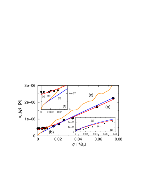
FIG. 2.: (colour) The longitudinal conductivity as deduced from the SAW $\Delta v_{s}/v_{s}$ at $\nu=1/2$ (here $a_{0}=9.79$ nm) corresponding to $n_{e}=6.27\times 10^{10}$ cm^-2 ($k_{F}^{\sc cf}=0.87/a_{0}$). Solid dots are experimental results by Willett, et al. [5], and (a), (b) and (c) have been calculated according to Eq. (4); for all three cases we have assumed $m_{b}=16\times m_{b}^{0}$, $m_{\star}=0.6\times m_{b}$, $d=10$ nm (for this value of $d$, $\sigma_{m}=3.57\times 10^{-7}$ ${=:}\sigma_{m}^{\rm th}$ according to Eq. (2)); in order to compare our results with those in Ref. [5], we have multiplied the theoretical $\sigma_{xx}(q)/\sigma_{m}$ by the value for $\sigma_{m}$ employed in this reference, namely [27] $\sigma_{m}=1.67\times 10^{-6}$ S. (a) has been determined with $\ell_{0}=0.6$ $\mu$m, (b) with $\ell_{0}=0.9$ $\mu$m and (c) with $\ell_{0}=2.4$ $\mu$m. (b) and (c) have been calculated with $\gamma^{\prime}=1$, while (a) has been obtained by following the procedure outlined in the text: taking the experimental result $\sigma_{xx}(q=0.004/a_{0})=0.44\times 10^{-6}$ S, we have obtained and used $\gamma^{\prime}=0.952$. Inset [A] is a focus on the small-$q$ region of the main diagram (the $q^{1/2}$-behaviour of (b) and (c) for $q\to 0$ is associated with $v(q)K_{00}(q,\omega)\propto q$ in this region), while inset [B] shows the counterparts of curves (a) and (b) for $m_{b}=m_{b}^{0}$, $m_{\star}=8\times m_{b}$ (for (a), $\gamma^{\prime}=1.008$).

In conclusion, by strictly adhering to the microscopic theory of CFs, we have established that the SAW-based experimental results by Willett and co-workers close to $\nu_{\rm e}=1/2$ can be remarkably accurately reproduced provided the electron band mass $m_{b}$ be substantially enhanced with respect to $m_{b}^{0}$; in this picture, the (observed) large value of the CF mass $m_{\star}$ follows from a subsequent reduction of $m_{b}$ (owing to quantum fluctuations) rather than a direct enhancement of $m_{b}^{0}$. We have further established that a finite mean-free path $\ell_{0}$ is essential to the experimentally-observed linearity in the SAW-deduced $\sigma_{xx}(q)$ in the range $1.56{\mathstrut{}_{\displaystyle{\sim}}^{\displaystyle<}}q{\mathstrut{}_{\displaystyle{\sim}}^{\displaystyle<}}7.68$ $\mu$m^-1, and that there exists no discrepancy between the theoretical and experimental values for $\sigma_{m}$.

I thank Professors D. E. Khmel’nitskiǐ and P. B. Littlewood for a discussion and Professor B. I. Halperin and Drs S. H. Simon and R. L. Willett for kindly clarifying some aspects concerning the empirical $\sigma_{m}$. With appreciation I acknowledge hospitality of Cavendish Laboratory.

REFERENCES

[1]
Q. Dai, et al.,
Phys. Rev. B 46, 5642 (1992).
[2]
A. Lopez, and E. Fradkin,
Phys. Rev. B 44, 5246 (1991).
[3]
B. I. Halperin, P. A. Lee, and N. Read,
Phys. Rev. B 47, 7312 (1993).
[4]
J. K. Jain,
Phys. Rev. Lett. 63, 199 (1989);
Phys. Rev. B 40, 8079 (1989);
Adv. Phys. 41, 105 (1992).
[5]
R. L. Willett, et al.,
Phys. Rev. B 47, 7344 (1993).
[6]
R. L. Willett, et al.,
Phys. Rev. Lett. 71, 3846 (1993).
[7]
W. Kang, H. L. Störmer, and L. N. Pfeiffer,
Phys. Rev. Lett. 71, 3850 (1993).
[8]
V. J. Goldman, B. Su, and J. K. Jain,
Phys. Rev. Lett. 72, 2065 (1994).
[9]
J. H. Smet, et al.,
Phys. Rev. Lett. 77, 2272 (1996).
[10]
R. L. Willett, K. W. West, and L. N. Pfeiffer,
Phys. Rev. Lett. 75, 2988 (1995).
[11]
R. R. Du, et al.,
Phys. Rev. Lett. 70, 2944 (1993).
[12]
R. R. Du, et al.,
Phys. Rev. Lett. 73, 3274 (1994).
[13]
H. C. Manoharan, M. Shayegan, and S. J. Klepper,
Phys. Rev. Lett. 73, 3270 (1994).
[14]
D. R. Leadly, et al.,
Phys. Rev. Lett. 72, 1906 (1994).
[15]
R. R. Du, et al.,
Solid State Commun. 90, 71 (1994).
[16]
P. T. Coleridge, et al.,
Phys. Rev. B 52, R11 603 (1995).
[17]
K. Park, and J. K. Jain,
Phys. Rev. Lett. 80, 4237 (1998).
[18]
I. V. Kukushkin, K. von Klitzing, and K. Eberl,
Phys. Rev. Lett. 82, 3665 (1999).
[19]
W. Kohn,
Phys. Rev. 123, 1242 (1961).
[20]
S. H. Simon,
Phys. Rev. B 54, 13878 (1996).
[21]
S. H. Simon, in Composite Fermions, edited by O. Heinonen
(World Scientific, Singapore, 1998).
[22]
S. H. Simon, and B. I. Halperin,
Phys. Rev. B 48, 17368 (1993);
S. H. Simon,
J. Phys. C 8, 10127 (1996).
[23]
S. C. Zhang,
Int. J. Mod. Phys. B 6, 25 (1992).
[24]
B. Farid,
arXiv:cond-mat/9912156; submitted.
[25]
M. H. Cohen, M. J. Harrison, and W. A. Harrison,
Phys. Rev. 117, 937 (1960).
[26]
A. D. Mirlin and P. Wölfle,
Phys. Rev. Lett. 78, 3717 (1997).