Statistical Properties of Eigenstates in three-dimensional Mesoscopic Systems with Off-diagonal or Diagonal Disorder

Abstract

The statistics of eigenfunction amplitudes are studied in mesoscopic disordered electron systems of finite size. The exact eigenspectrum and eigenstates are obtained by solving numerically Anderson Hamiltonian on a three-dimensional lattice for different strengths of disorder introduced either in the potential on-site energy (“diagonal”) or in the hopping integral (“off-diagonal”). The samples are characterized by the exact zero-temperature conductance computed using real-space Green function technique and related Landauer-type formula. The comparison of eigenstate statistics in two models of disorder shows sample-specific details which are not fully taken into account by the conductance, shape of the sample and dimensionality. The wave function amplitude distributions for the states belonging to different transport regimes within the same model are contrasted with each other as well as with universal predictions of random matrix theory valid in the infinite conductance limit.

The disorder induced localization-delocalization (LD) transition in solids has been one of the most vigorously pursued problems in condensed matter physics since the seminal work of Anderson. [1] In thermodynamic limit, strong enough disorder generates a zero-temperature critical point in $d>2$ dimensions [2] as a result of quantum interference effects (in $d\leq 2$ even weakly disordered metal turns into an Anderson insulator for sufficiently large sample size). Thus, research in the “pre-mesoscopic” era [3] was mostly directed toward the viewpoint provided by the theory of critical phenomena. [4] The advent of mesoscopic quantum physics [5] has unearthed large fluctuations, induced by quantum coherence and randomness of disorder, [6] of various physical quantities [7] (e.g., conductance, local density of states, current relaxation times, etc.), even well into the delocalized phase. Thus, complete understanding of the LD transition requires to examine full distribution functions of relevant quantities. [8] Especially interesting are the deviations of their asymptotic tails, a putative signature of incipient localization, [7] from the (usually) Gaussian distributions expected in the limit of infinite dimensionless conductance $g=G/G_{Q}$ ($G_{Q}=2e^{2}/h$ is the conductance quantum).

This paper presents the study of such type—numerical computation of the statistics of eigenfunction amplitudes in finite-size three-dimensional (3D) nanoscale (composed of $\sim 1000$ atoms) mesoscopic disordered conductors. The 3D conductors are often “neglected” in favor of the more popular and tractable playgrounds—two-dimensional systems (2D), where one can study states resembling 3D critical wave functions in a wide range of systems sizes and disorder strengths, [9, 10] or quasi one-dimensional systems [11] where analytical techniques [12, 13] can handle even non-perturbative phenomena [14] (like the ones at small $g$). For example, in $d=2+\epsilon$ dimensions LD transition occurs at weak disorder (weak-coupling regime of the corresponding field-theoretical description [12]), while in $d\geq 3$ small parameter needed for analytical treatment is lacking. In 3D systems critical eigenfunctions, exhibiting multifractal scaling, [6] are expected only at the mobility edge $E_{c}$ which separates extended and localized states inside the energy band.

The essential physics of disordered conductors is captured by studying the quantum dynamics of a non-interacting (quasi)particle in a random potential. This problem is classically non-integrable, thereby exhibiting quantum chaos. The concepts unifying disordered electron physics with the standard ‘clean’ (i.e., without stochastic disorder) examples of quantum chaos [15] come from statistical approaches to the properties of energy spectrum and corresponding eigenstates, which cannot be computed analytically. While level statistics of disordered systems have been explored to a great extent, [16, 17] investigation of the statistics of eigenfunctions has been initiated only recently. [9] These studies are not only revealing peculiar spectral properties of random Hamiltonians, but are relevant for the thorough understanding of various unusual features of quantum transport in diffusive metallic conductors (including the ones which are proximity coupled to a superconductor [18]). The standard examples are long-time tails in the relaxation of current [19] or log-normal tails (in $d=2+\epsilon$) of the distribution function of mesoscopic conductances. [7] Distribution of eigenfunction amplitudes is found to be relevant for tunneling measurements on quantum dots probing the coupling to external leads, which depends sensitively on the local properties of wave functions. [20]

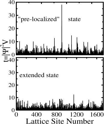
FIG. 1.: An example of eigenstates in the band center of a delocalized phase. The average conductance at half filling is $g(E_{F}=0)\approx 17$, entailing anomalous rarity of the “pre-localized” states. The disordered conductor is modeled by an Anderson model with diagonal disorder $W_{\rm DD}=4$ on a simple cubic lattice $12^{3}$. For plotting of the eigenfunction values in 3D, the sites ${\bf m}$ are mapped onto the lattice site numbers $\in\{1,...,1728\}$ in a lexicographic order, i.e., ${\bf m}\equiv(m_{x},m_{y},m_{z})\mapsto 144(m_{x}-1)+12(m_{y}-1)+m_{z}$.

Experiments which are the closest to directly delving into the microscopic structure of quantum chaotic or disordered wave functions exploit the correspondence between the Schrödinger and Maxwell equations in microwave cavities. [21]

The study of fluctuations and correlations of eigenfunction amplitudes [9, 22] in mesoscopic systems has led to a concept of the so-called “pre-localized” states. [7, 19, 23] In 3D delocalized phase, this notion refers to the states which have sharp amplitude peaks on the top of an extended background. [24] These kind of states appear even in the diffusive, $\ell\ll L<\xi$, metallic ($g\gg 1$) regime, but are anomalously rare in such samples (here $\ell$ is the elastic mean free path and $\xi$ is the localization length). In order to get “experimental” feeling for the structure of states with unusually high amplitude spikes, an example is given in Fig. 1; this state is found in a special realization of quenched disorder (out of many randomly generated impurity configurations) inside the sample characterized by large average conductance. Thus, pre-localized states are putative precursors of LD transition and determine asymptotics of some of the distribution functions [6, 9] studied in open or closed mesoscopic systems. In $d\leq 2$, where all states are considered to be localized, [4] pre-localized states have anomalously short localization radius [9] when compared to “ordinary” localized states in low-dimensional systems. They underlie [23] the multifractal scaling in weakly localized ($g\gg 1$) 2D conductors of size $L$ smaller than exponentially large $\xi$ (which plays the role of a phase transition correlation length [6] $\xi_{c}=\xi$ in $d\leq 2$). In 3D, the correlation length $\xi_{c}$ (defined as the size of a hypercube for which [6] $g(\xi_{c})={\mathcal{O}}(1)$) is always microscopic ($\xi_{c}\sim\lambda_{F}$) in good metallic samples, and no multifractal scaling is expected. The appearance of small regions inside disordered solids where eigenstates can have large amplitudes seems to be a “strongly pronounced” analog [10, 21] of the phenomenon of scarring [25] (anomalous enhancement or suppression of quantum chaotic wave function intensity on the unstable periodic orbits in the corresponding classical system) introduced in the guise of generic quantum chaos.

In general, the study of properties of wave functions on a scale smaller than $\xi$ should probe quantum effects causing evolution of extended into localized states upon approaching the LD critical point. In the marginal two-dimensional case, the divergent (in the limit $L\rightarrow\infty$) weak localization (WL) correction [26] to the semiclassical Boltzmann conductivity provides an explanation of localization in terms of the interference between two amplitudes to return to initial point along the same classical path in the opposite directions. [27] This simple quantum interference effect leads to a coherent backscattering (i.e., suppression of conductivity) in a time-reversal invariant systems without spin-orbit interaction. However, in 3D systems WL correction is not “strong” enough to provide a full microscopic picture of complicated quantum interference processes which are responsible for LD transition, and facilitate the expansion of quantum intuition.

The paper presents the statistics of eigenfunction intensities $|\Psi_{\alpha}({\bf r})|^{2}$ in isolated 3D mesoscopic conductors characterized by two different types of microscopic disorder. Numerical methods employed here make it possible to treat phenomena in both semiclassical (described by Bloch-Boltzmann formalism and perturbative quantum corrections [12]) and fully quantum transport regime (dominated by non-perturbative effects, where semiclassical concepts, like $\ell$, loose their meaning [28]), as well as in the crossover realm. Since mesoscopic physics has provided efficient techniques [29] for “measuring” exactly the transport properties of finite-size samples on the computer, this study connects the eigenstates statistics of a closed sample to its zero-temperature conductance. The statistical properties of eigenstates are described by the disorder-averaged distribution function [14, 23]

$$f(t)=\frac{1}{\rho(E)N}\left\langle\sum_{{\bf r},\alpha}\delta(t-|\Psi_{\alpha}({\bf r})|^{2}V)\delta(E-E_{\alpha})\right\rangle,$$ (1)

on $N$ discrete points ${\bf r}$ inside a sample of volume $V$. Here $\rho(E)=\langle\sum_{\alpha}\delta(E-E_{\alpha})\rangle$ is the mean level density at energy $E$. Averaging over disorder is denoted by $\langle\ldots\rangle$. Normalization of eigenstates gives $\bar{t}=\int dt\,t\,f(t)=1$. A finite-size disordered sample is modeled by a tight-binding Hamiltonian (TBH) with nearest neighbor hopping integral $t_{{\bf m}{\bf n}}$

$$\hat{H}=\sum_{\bf m}\varepsilon_{\bf m}|{\bf m}\rangle\langle{\bf m}|+\sum_{\langle{\bf m},{\bf n}\rangle}t_{{\bf m}{\bf n}}|{\bf m}\rangle\langle{\bf n}|,$$ (2)

on a simple cubic lattice $16\times 16\times 16$ of lattice constant $a$. Each site ${\bf m}$ contains a single $s$-orbital $\langle{\bf r}|{\bf m}\rangle=\psi({\bf r}-{\bf m})$. Periodic boundary conditions are chosen in all directions. In a random hopping (RH) model the disorder is introduced by taking the off-diagonal matrix elements to be a uniformly distributed random variable, [30] $1-2W_{\text{RH}}<t_{{\bf m}{\bf n}}<1$, while diagonal elements are zero $\varepsilon_{\bf m}=0$. The strength of the disorder is measured by $W_{\text{RH}}$. The other system studied is described by a diagonally disordered (DD) Anderson model with potential energy $\varepsilon_{\bf m}$ on site ${\bf m}$ drawn from the uniform distribution, $-W_{\text{DD}}/2<\varepsilon_{\bf m}<W_{\text{DD}}/2$, and $t_{{\bf m}{\bf n}}=1$ is the unit of energy. The Hamiltonian (2) is a real symmetric matrix because time-reversal symmetry is assumed. The results for $f(t)$ in the samples described by the RH and DD Anderson models are shown on Figs. 2, 3 and Fig. 4, respectively. Although some of the samples are characterized by similar values of conductance, the eigenstates in the two models show different statistical behavior.

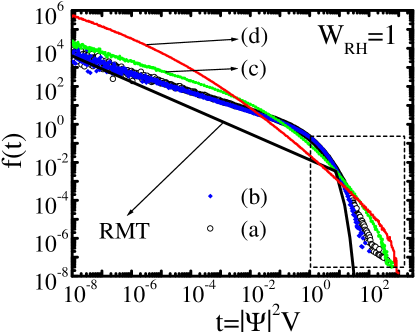
FIG. 2.: Statistics of wave function intensities in the RH Anderson model, with $W_{\text{RH}}=1$, on a simple cubic lattice $16^{3}$. The distribution function $f(t)$ in Eq. (1) is computed for the states around the following energies: (a) $E=0$, (b) $E=1.5$, (c) $E=2.55$, and (d) $E=2.75$. Disorder averaging is performed over $N_{\text{Ens}}=40$ different samples. The Porter-Thomas distribution (3) is denoted by RMT. The part of the distributions inside the dashed box in enlarged on Fig. 3.

In what follows the meaning of these findings is explained in the context of statistical approach to quantum systems with non-integrable classical dynamics. In particular, the results are compared to the universal predictions of random matrix theory (RMT).

In the statistical approach [17] of RMT, the Hamiltonian of a quantum chaotic system is replaced [31] by a random matrix drawn from an ensemble defined by the symmetries under time-reversal and spin-rotation. This leads to the Wigner-Dyson (WD) statistics for eigenvalues and Porter-Thomas (PT) distribution for eigenfunction intensities. For the Gaussian orthogonal ensemble (GOE), relevant for studies of time-reversal-invariant Hamiltonians like (2), the PT distribution is given by

$$f_{\text{PT}}(t)=\frac{1}{\sqrt{2\pi t}}\exp(-t/2).$$ (3)

The function $f_{\text{PT}}(t)$ is plotted as a reference in Figs. 2, 3 and Fig. 4. The predictions of RMT are universal, depending only on the symmetry properties of the relevant ensemble. They apply to the statistics of real disordered systems [33] in the limit $g\rightarrow\infty$ ($g=\pi E_{\text{Th}}/\Delta$, where $\Delta=1/\rho(E)$ is the mean energy level spacing and $E_{\text{Th}}=\hbar{\mathcal{D}}/L^{2}$ is the Thouless energy, set by the classical diffusion across a sample of size $L$ with diffusion constant ${\mathcal{D}}$). The spectral correlations in RMT are determined by logarithmic level repulsion which is independent of true dynamics. [17]

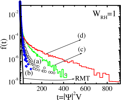
FIG. 3.: Statistics of wave function intensities in the RH Anderson model, with $W_{\text{RH}}=1$, on a simple cubic lattice with $N=16^{3}$ sites. This Figure plots the same distributions $f(t)$ as the ones plotted in Fig. 2, in the range defined by the dashed square in Fig. 2. The same labels apply to both Figures.

All sample-specific details are absorbed into the mean level spacing [17] $\Delta$. Also, the level correlations are independent of the eigenstate correlations. The RMT answer (3) for the distribution function (1) was derived by Porter and Thomas [34] by assuming that the coordinate-representation eigenstate $\langle{\bf r}|\Psi_{\alpha}\rangle$ in a disordered (or classically chaotic system) is a Gaussian random variable. The behavior of $\Psi_{\alpha}({\bf r})$, even within the framework of RMT, is simple only in the systems with unbroken or completely broken time-reversal symmetry [the only difference between the two limiting ensembles is the functional form of $f(t)$]. [35] Thus, RMT implies statistical equivalence of eigenstates which equally test the random potential all over the sample—typical wave function has more or less uniform amplitude $1/\sqrt{V}$, up to inevitable Gaussian fluctuations.

Microscopic theory brings corrections to the RMT results in the

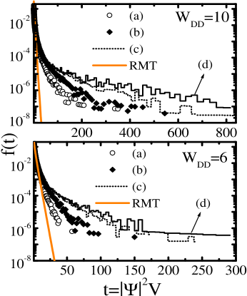
FIG. 4.: Statistics of wave function intensities in the DD Anderson model on a simple cubic lattice $16^{3}$. The distribution function $f(t)$, Eq. (1), is computed for the states around following energies. Upper panel, $W_{\text{DD}}=10$: (a) $E=0$, (b) $E=6.0$, (c) $E=7.45$, and (d) $E=7.85$. Lower panel, $W_{\text{DD}}=6$: (a) $E=0$, (b) $E=4.1$, (c) $E=6.56$, and (d) $E=6.7$. Disorder averaging is performed over $N_{\text{Ens}}=40$ different samples. The Porter-Thomas distribution (3) is denoted by RMT.

case of samples with finite $g$. In the finite-size systems level statistics follow RMT predictions in the ergodic regime, i.e., on the energy separation scale smaller than $E_{\text{Th}}$. Non-universal corrections to the spectral statistics [36] or eigenfunction statistics [9, 23, 37] (which describe the long-range correlations of wave functions) depend on dimensionality, shape of the sample, and conductance $g$. These deviations from RMT predictions grow with increasing disorder (i.e., lowering of $g$). At the LD transition wave functions acquire multifractal properties, while the critical level statistics become scale-independent. [38] For strong disorder or, at fixed disorder, for energies $|E|$ above the mobility edge $|E_{c}|$, wave functions are exponentially localized. The simple (and usually invoked) picture is that of a wave function which decays as $\Psi(r)=p(r)\exp(-r/\xi)$ from its maximum centered at some point inside the sample of size $L>\xi$. Here $p(r)$ is a random function and approximately spherical symmetry of decay is assumed. Since two states close in energy are localized at different points in space, there is almost no overlap between them. Therefore, the levels become uncorrelated and obey Poisson statistics. If $p(r)=c$ is simplified to a normalization constant, the distribution function of intensities is given by

$$f_{\xi}(t) = \frac{4\pi}{V}\int\limits_{0}^{L/2}dr\,r^{2}\delta(t-|\Psi(r)|^{2}V)=\frac{\pi\xi^{3}}{4V}\frac{\ln^{2}(c^{2}V/t)}{t},$$ (4)

$$c^{2} = \frac{2}{\pi\xi^{3}}\left[1-\left(1+\frac{L}{\xi}+\frac{L^{2}}{2\xi^{2}}\right)e^{-L/\xi}\right]^{-1},$$ (5)

where a spherically symmetric sample of radius $L/2$ is assumed. In the localized phase $\xi\ll L$, $f_{\xi}(t)$ is expected to be insensitive to the assumed shape of the sample, and is determined by the ratio of these two relevant length scales.

The distribution function $f(t)$ is equivalently given in term of its moments $b_{q}=\int dt\,t^{q}\,f(t)$ (this statement is not rigorous since examples of different distribution functions which possess exactly the same sets of moments are encountered in various statistical problems [39, 40]). For GOE, the PT distribution (3) has moments $b_{q}^{\text{PT}}=2^{q}V^{-q+1}\Gamma(q+1/2)/\Gamma(1/2)$. They are related to the moments $I_{\alpha}(q)=\int d{\bf r}\,|\Psi_{\alpha}({\bf r})|^{2q}$ of the wave function intensity.

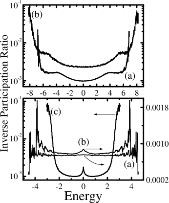
FIG. 5.: Inverse Participation Ratio $I(2)$ ,averaged over both 40 different conductors and small energy bins, of eigenstates in the RH and DD Anderson models on a simple cubic lattice with $N=16^{3}$ sites. Top: diagonal disorder with (a) $W_{\text{DD}}=6$, and (b) $W_{\text{DD}}=10$. Bottom: off-diagonal disorder with (a) $W_{\text{RH}}=0.25$, (b) $W_{\text{RH}}=0.375$, and (c) $W_{\text{RH}}=1$.

In the universal regime $g\rightarrow\infty$ wave functions cover the whole volume with only short-range correlations (on the scale $|{\bf r}_{1}-{\bf r}_{2}|\lesssim\ell$) persisting between $\Psi_{\alpha}({\bf r}_{1})$ and $\Psi_{\alpha}({\bf r}_{2})$. This means that integration in the definition of $I_{\alpha}(q)$ provides self-averaging, and $I_{\alpha}(q)$ does not fluctuate in the universal limit, [37] i.e., $I_{\alpha}(q)=b_{q}^{\text{PT}}$. On the other hand, at finite $g$ spatial correlations of wave function amplitudes at distances comparable to the system size are non-negligible. Therefore, $I_{\alpha}(q)$ fluctuates from state to state and from sample to sample. [22, 41] Although these long-range spatial correlations necessitate to study the full distribution function [37, 41] of $I_{\alpha}(q)$, for the subsequent analysis in this study it is enough to use an ensemble average of $I_{\alpha}(q)$, i.e., following Wegner [42]

$$I(q)=\Delta\left\langle\sum_{{\bf r},\alpha}\,|\Psi_{\alpha}({\bf r})|^{2q}\delta(E-E_{\alpha})\right\rangle.$$ (6)

The moment $I_{\alpha}(2)$ is usually called inverse participation ratio (IPR). It is a one-number measure of the degree of localization (i.e., it measures the portion of space where the amplitude of the wave function differs markedly from zero). This becomes obvious from the scaling properties of the average moments $I(q)$ with respect to the system size

$$I(q)\propto\cases{L^{-d(q-1)}\ \ \ \ \ \ \ \ {\text{ metal}},\cr L^{0}\ \ \ \ \ \ \ \ \ \ \ \ \ {\text{insulator}},\cr L^{-d^{*}(q)(q-1)}\;\;\;\,{\text{critical}}.\cr}$$ (7)

Here $d^{*}(q)<d$ is the fractal dimension. Its dependence on $q$ is the hallmark of multifractality of wave functions. The multifractal wave functions are delocalized, but extremely inhomogeneous occupying only an infinitesimal fraction of the sample volume in thermodynamic limit. The IPR is affected by mesoscopic fluctuations which scale in metallic samples as [22] $\delta I_{\alpha}(2)\sim 1/g^{2}\propto L^{4-2d}$. In the critical region ($g\sim 1$) fluctuations [22] are of the same order as the average value, which is then not enough to characterize the critical eigenstates (even though multifractal wave function extend throughout the whole sample, their IPR is not self-averaging [41]).

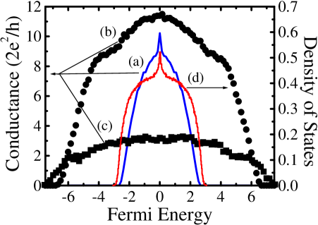
FIG. 6.: Conductance and density of states in the RH and DD Anderson models on a simple cubic lattice $16^{3}$: RH disorder, (a) and (d), of strength $W_{\text{RH}}=1$ (mobility edge is at $|E_{c}|\simeq 2.53$); diagonal disorder of strength (b) $W_{\text{DD}}=6$ ($|E_{c}|\simeq 6.5$), and (c) $W_{\text{DD}}=10$ ($|E_{c}|\simeq 7.4$). Disorder averaging is performed over $N_{\text{Ens}}=20$ different samples for conductance and $N_{\text{Ens}}=40$ for DoS.

I use $I(2)$ as a rough guide in selecting eigenstates with different properties in the delocalized phase (Fig. 5). The second parameter used in the selection procedure is the conductance $g(E_{F})$ computed for a band filled up to the Fermi energy $E_{F}$ equal to the state eigenenergy (see Fig. 6). The conductance as a function of band filling allows one to delineate delocalized from localized phase as well as to narrow down the critical region around LD transition point (which is defined by $g(E_{c})\sim 1$). Upon inspection of these two parameters, a small window is placed around chosen energy, and $f(t)$ is computed for all eigenenergies whose eigenvalues fall inside the window. This provides more detailed information on the structure of eigenstates than is encoded in IPR.

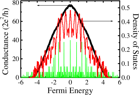
FIG. 7.: Conductance and density of states in the RH Anderson models on a simple cubic lattice $16^{3}$. The strenght of the RH disorder is $W_{\rm RH}=0.25$, which is so weak that features of a discrete spectrum of a finite-size lattice are still visible in the disorder-averaged DOS. Sharp lines correspond to the DoS of a clean system on the same lattice (scaled by $1/10$ for clarity). Disorder averaging is performed over $N_{\text{Ens}}=20$ different samples for conductance and $N_{\text{Ens}}=40$ for DoS.

The average IPR for both RH and DD Anderson model is shown in Fig. 5. The models with random hopping have been around for a long time, [43, 44] but have attracted considerable attention only recently, inasmuch as they show a disorder induced quantum critical point in less than three dimensions, [30, 45, 46, 47] where delocalization occurs in the band center. Furthermore, several models used for strongly correlated electron systems share similar mathematical structure with the random hopping 2D models formulated in the framework of (non-interacting) disorder electron physics. [48] Real solids which could be described by TBH (2) with off-diagonal disorder include doped semiconductors, [44] such as P-doped Si, where hopping integrals $t_{\bf mn}$ vary exponentially with the distances between the orbitals they connect, while diagonal on-site energies $\varepsilon_{\bf m}$ are nearly constant. The behavior of low-dimensional RH Anderson model goes against the standard mantra of the scaling theory of localization for non-interacting systems [4] that all electron states are localized in $d\leq 2$ for arbitrarily weak disorder. The possibility of delocalization transition in one dimension [49] goes back to the work of Dyson [50] on glasses. Also, the scaling theory for quantum wires with off-diagonal disorder requires two parameters [51] which depend on the microscopic model, thus breaking the celebrated universality in disordered electron problems. In 3D case explored here, the states in the band center are less extended than other delocalized states inside the band (Fig. 5). However, the off-diagonal disorder is not strong enough [52] to localize all states in the band, in contrast to the usual case of diagonal disorder where whole band becomes localized [53] for $W_{\text{DD}}^{c}\gtrsim 16.5$.

The mobility edge for the strongest RH disorder $W_{\text{RH}}=1$, as well as for DD models, is found by looking at an exact zero-temperature static conductance. This quantity (which is a Fermi surface property) is computed from the Landauer-type formula [54]

$$g(E_{F})=\text{Tr}\,[{\bf t}(E_{F}){\bf t}^{{\dagger}}(E_{F})],$$ (8)

where transmission matrix ${\bf t}(E_{F})$ is expressed in terms of the real-space (lattice) Green functions [29, 55] for the sample attached to two clean semi-infinite leads. To study the conductance in the whole band of the DD model, $t_{{\bf m}{\bf n}}=1.5$ is used [55] for the hopping integral in the leads. This mesoscopic computational technique “opens” the sample, thereby smearing the discrete levels of an initially isolated system. Thus, the spectrum of sample+leads=infinite system becomes continues and conductance can be calculated at any $E_{F}$ inside the band. However, the computed conductance, for not too small disorder [55, 56] or coupling to the leads [57] (which are of the same transverse width as the sample [56]) is practically equal to the “intrinsic” conductance $g=\pi E_{\rm Th}/\Delta$ determined by the spectral properties of a closed sample.

The conductance and density of states (DoS)

$$N(E)=2\frac{\rho(E)}{V},$$ (9)

are plotted in Fig. 6 for the samples whose eigenstates are investigated (the factor of two is for spin degeneracy). The DoS is obtained from the histogram of the number of eigenvalues which fall into equally spaced energy bins along the band. The conductance and DoS of the RH model have a peak at $E=0$, which becomes a logarithmic singularity in the limit of infinite system size. [50] To get an insight into the “general weakness” of the off-diagonal disorder, Fig. 7 plots $g(E_{F})$ and $N(E)$ for the low $W_{\text{RH}}=0.25$. In this case $N(E)$ still resembles the DoS of a clean system, even after ensemble averaging. On the other hand, the conductance is a smooth function of energy since discrete levels of an isolated sample are broadened by the coupling to leads. The same is true for the DoS computed from the imaginary part of the Green function for an open system. The mobility edge is absent at low RH disorder ($W_{\rm RH}=0.25$ and $W_{\rm RH}=0.375$) for system sizes $L\leq 16a$. This means that localization length $\xi$ is greater than $16a$ for all energies inside the band of these systems. For other samples on Fig. 6 the mobility edge appears inside the band. This is clearly shown for $W_{\rm RH}=1$ case where band edge $E_{b}$ ($N(E_{b})=0$) differs from $E_{c}$. The mobility edge is located at the minimum energy $|E_{c}|$ for which $g(E_{c})$ is still different from zero. The conductance of finite samples is always finite, although exponentially small at $|E_{F}|>|E_{c}|$. The approximate values of $|E_{c}|$ listed in Fig. 6 are such that conductance satisfies: $g(E_{F})<0.1$, for $|E_{F}|>|E_{c}|$; typically $g(E_{c})\in(0.2,0.5)$ is obtained, like in the recent detailed studies [58] of conductance properties at $E_{c}$. Thus found $E_{c}$ is virtually equal to the true mobility edge, which is properly defined only in thermodynamic limit (and usually obtained from some numerical finite-size scaling procedure [2]). Namely, the position of mobility edge extracted in this way will not change [59] when going to larger system sizes if $\xi<L$ for all energies $|E|>|E_{c}|$.

The distribution $f(t)$ of eigenfunction intensities has been studied analytically for diffusive conductors close to the universal RMT limit (where conductance is large and localization effects are small) in Refs. [9, 23] using the supermatrix $\sigma$-model (NLSM), [12] or by means of a “direct optimal fluctuations method” of Ref. [60]. Numerical studies of statistics of eigenstates in DD Anderson model were conducted in 2D for all disorder strengths, [10] while in 3D the focus has been on the states appearing in the semiclassical transport regime where comparison with analytical predictions (parameterized by semiclassical quantities, like $k_{F}\ell$) can be made in the regions of small [61] and large [62] deviations of $f(t)$ from PT distribution. Here I show how $f(t)$ evolves with the strength of (different types of) disorder in 3D samples, where genuine LD transition occurs in the strong coupling regime of the corresponding field-theoretical formulation.

In the weakly disordered ($k_{F}\ell\gg 1$) metallic ($g\gg 1$) conductors pre-localized states are extremely rare. For example, in an ensemble of 20 000 samples ($W_{\rm DD}=4$), whose typical transport properties are well-described by semiclassical theories, only four states would show up in the band center which exhibit similar amplitude splashes like the one in Fig. 1. Thus, to get a far tail (where deviations from PT distribution are large) of $f(t)$ in such conductors one has to search through enormous ensemble and locate special configurations of a random potential. [62] The maximum wave function amplitudes which can be observed in this pursuit are, plausibly, determined by the strength of disorder, i.e., conductance $g$. It is, however, interesting that tails at small but finite $g$ in the strong disorder (like $W_{\rm DD}=10$) can be longer than the tails of states in the localized phase, where $g$ is vanishingly small, for $|E|>|E_{c}|$ at some smaller fixed disorder (like in the case of $W_{\rm DD}=6$; compare the two panels in Fig. 4 using respective conductances from Fig. 6). For strong enough disorder long tails of $f(t)$ are found, even by investigating small ensembles of disordered conductors (as shown below), since the frequency of appearance of pre-localized states is greatly enhanced (while system is still on the delocalized side of LD transition).

The complete eigenproblem of a single particle random Hamiltonian is solved exactly by numerical diagonalization. Then, $f(t)$ is computed as a histogram of intensities for the chosen eigenstates in: delocalized ($|E|<|E_{c}|$), localized phase ($|E|>|E_{c}|$), and critical region around the mobility edge $|E_{c}|$. The two delta functions in Eq. (1) are approximated by a box function $\bar{\delta}(x)$. The width of $\bar{\delta}(E-E_{\alpha})$ is small enough at a specific energy that $\rho(E)$ is constant inside that interval. For each sample, 5–10 states are picked by the energy bin, which effectively provides additional averaging over the disorder (according to ergodicity [17] in RMT). The amplitudes of wave functions are sorted in the bins defined by $\bar{\delta}(t-|\Psi_{\alpha}({\bf r})|^{2}V)$ whose width is constant on a logarithmic scale. The function $f(t)$ is computed at all points inside the sample, i.e., $N=16^{3}$ in Eq. (1).

The evolution of $f(t)$, when sweeping the band through the interesting states, is plotted in Figs. 2, 3 for the RH disordered sample. Since pre-localized states generate slow decay of $f(t)$ at high wave function intensities (where PT distribution is negligible), [12] this region is enlarged on Fig. 3. This is obvious from the pre-localized example in Fig. 1 where state with large amplitude spikes, highly unlikely in the framework of RMT, was found in a very good metal. The same is trivially true for the localized states which determine extremely long tails of $f_{\xi}(t)$. Thus, the long asymptotic tails of $f(t)$, appreciably deviating from PT distribution, are signaling the onset of localization. It is interesting that states in the band center of RH model, which define the largest zero-temperature conductance $[g(E_{F}=0)\approx 10.2$, Var $g(E_{F}=0)\approx 0.63]$, are in fact mostly pre-localized. Moreover, both the frequency of their appearance and high amplitude splashes resemble the situation at criticality (NLSM-type calculation [47] shows that 3D wave functions, sufficiently close to the band center, are always extended for any disorder strength). It might be conjectured that these pre-localized states would generate multifractal scaling of IPR in the band center. This result, together with the DoS and conductance from Figs. 6, 7, shows that phenomena in the band center of 3D conductors with off-diagonal disorder are as intriguing as their much studied counterparts in low-dimensional systems. [30, 45, 46] The origin of these phenomena can be traced back to a special sublattice, or “chiral”, [44, 63] symmetry obeyed by TBH (2) with random hopping and constant on-site energy (leading to an eigenspectrum which for $E_{\alpha}$ contains $-E_{\alpha}$, with a special role played by $E=0$). In the $W_{\text{RH}}=0.25$ and $W_{\text{RH}}=0.375$ cases all states are extended. Their $f(t)$ looks similar to the distribution function for the delocalized states at $E=1.5$ in the sample characterized by $W_{\text{RH}}=1$. The distribution function $f_{\xi}(t)$ defined in Eq. (4) fits reasonably well the numerical $f(t)$ generated by the states around $E=2.75$, where $\xi\simeq 1.2a$ is extracted for the localization length. Thus, one can measure approximately $\xi$ in this way [10] even though the structure of localized eigenstates can be more complicated [2] than the simple radially symmetric exponential decay used to derive $f_{\xi}(t)$ [e.g., in the case of DD disorder $\xi\simeq 1.3a$ is obtained for examined localized states in Fig. 4 for $W_{\rm DD}=10$ ensemble, while corresponding states in $W_{\rm DD}=6$ ensemble seem to be too close to the mobility edge to follow $f_{\xi}(t)$].

The same statistical analysis is performed for the eigenstates of DD Anderson model—a “standard model” in the localization theory. Figure 4 plots $f(t)$ at specific energies $E_{i}$ in samples characterized by different conductances $g(E_{F}=E_{i})$. The conductance $g(E=0)$ of TBH with $W_{\text{DD}}=6$ is numerically close to the conductance of RH disordered samples with $W_{\text{RH}}=1$. Nevertheless, comparison of the corresponding distribution functions reveals disorder-dependent features [9] which are beyond universal corrections (i.e., independent of the details of random potential) accounted by the properties of a classical diffusion operator [14, 37] (the spectrum of $-{\mathcal{D}}\nabla^{2}$, with appropriate boundary conditions, depends on $g$, shape of the sample and dimensionality; note that conductors at $W\simeq 6$ with half-filled band lie on the boundary of applicability of such semiclassical concepts [28]). To get the far tail of the eigenstate statistics in the band center a much larger statistics is needed than used here. [62] This then makes the observed $f(t)$ in a special case of the band center of $W_{\text{RH}}=1$ disordered conductor even more spectacular because of very large amplitudes found in the small ensemble of conductors. Thus, the strong dependence on the microscopic details of random potential demonstrated in this study is somewhat different from the disorder-specific short length scale (“ballistic” [9]) contributions [9, 62] to the standard picture of diffusive NLSM. Namely, here it seems that special features of off-diagonal disorder in the band center generate completely different functional form of the far tail, and not just some disorder-specific values of the parameters [9, 62] in the exp-log-cube asymptotics. [9, 23, 60].

In both models, all computed $f(t)$ intersect PT distribution (from below) around $6\lesssim t\lesssim 10$, and then develop tails far above PT values. The length of the tails is defined by the largest amplitude exhibited in the pre-localized state (like that in Fig. 1). For strong DD, $W_{\text{DD}}=10$, the conductance $g(E_{F})$ is smaller than $3.5$. In this regime transport becomes “intrinsically diffusive”, [28] but one can still extract resistivity from the approximate Ohmic scaling of disorder-averaged resistance [28] (for those fillings where [64] $g(E_{F})>2$). However, the close proximity to the critical region $g\sim 1$ induces long tails of $f(t)$ at all energies throughout the band—a sign of increased frequency of appearance of highly inhomogeneous states. This provides an insight into the microscopic structure of eigenstates which carry the current in a non-semiclassical transport regime [12] (characterized by the lack of simple intuitive concepts, like mean free path $\ell$, since unwarranted use of the Boltzmann theory would give [28] $\ell<a$ in this transport regime although the sample is still far away from the LD transition).

In conclusion, the statistics of eigenstates in 3D mesoscopic conductors, modeled by the tight-binding Hamiltonian on the finite-size simple cubic lattice, have been studied. The disorder is introduced either in the potential energy (diagonal) or in the hopping integrals (off-diagonal). Also calculated are the average inverse participation ratio of eigenfunctions and the exact zero-temperature conductance as a function of Fermi energy. This comprehensive set of parameters makes it possible to compare the eigenstates in nanoscale samples with different types of disorder, but characterized by similar values of conductance. Disorder-specific details, which are not parameterized by the conductance alone, are found. This is in spite of the fact that dimensionality, shape of the sample, and conductance are expected to determine the finite-size corrections to the universal predictions of random matrix theory, at least in the samples which are in the semiclassical transport regime. The appearance of states with large amplitude spikes on the of top of RMT like background is clearly demonstrated even in good metals. At criticality, the proliferation of such “pre-localized” states is directly related to the extensively studied multifractal scaling of IPR. However, even in the delocalized phase with good metallic properties ($g\gg 1$), where the correlation length [6] $\xi_{c}\sim\lambda_{F}$ defined by the sample conductance $g(\xi_{c})\sim 1$ is microscopic ($L<\xi_{c}$ would naturally account for the multifractal scaling, [6] like in 2D), pre-localized state with unexpectedly high amplitudes are found in the band center of random hopping disordered systems. They are inhomogeneous enough to generate extremely long tails of the distribution of eigenfunction amplitudes, akin to the ones observed at criticality.

Inspiring discussions with V. Z. Cerovski are acknowledged. Valuable guidance have been provided by P. B. Allen. The important improvements of the initial cond-mat preprint have resulted from criticism provided by B. Shapiro and I. E. Smolyarenko. This work was supported in part by NSF grant no. DMR 9725037.

${\ddagger}$ Present address: Department of Physics, Georgetown University, Washington, DC 20057-0995.

REFERENCES

- [1] P. W. Anderson, Phys. Rev. 109, 1492 (1958).
- [2] B. Kramer and A. MacKinnon, Rep. Prog. Phys. 56, 1469 (1993).
- [3] P.A. Lee and T.V. Ramakrishnan, Rev. Mod. Phys. 57, 287 (1985).
- [4] E. Abrahams, P. W. Anderson, D. C. Licciardello, and T. V. Ramakrishnan, Phys. Rev. Lett. 42, 673 (1979).
- [5] Mesoscopic Quantum Physics, edited by E. Akkermans, J.-L. Pichard, and J. Zinn-Justin, Les Houches, Session LXI, 1994 (North-Holland, Amsterdam, 1995).
- [6] M. Janssen, Phys. Rep. 295, 1 (1998).
- [7] B. L. Altshuler, V. E. Kravtsov, and I. V. Lerner, in Mesoscopic phenomena in solids, edited by B. L. Altshuler, P. A. Lee, and R. A. Webb (North-Holland, Amsterdam, 1991).
- [8] B. Shapiro, Phil. Mag. B 56, 1031 (1987).
- [9] For a recent comprehensive review see: A. D. Mirlin, Phys. Rep. 326, 259 (2000).
- [10] K. Müller, B. Mehlig, F. Milde, and M. Schreiber, Phys. Rev. Lett. 78, 215 (1997).
- [11] V. Uski, B. Mehlig, R. A. Römer, and M. Schreiber, Phys. Rev. B 62, R7699 (2000).
- [12] K. B. Efetov, Supersymmetry in Disorder and Chaos (Cambridge University Press, Cambridge, 1997).
- [13] P.W. Brouwer and K. Frahm, Phys. Rev. B 53, 1490 (1996).
- [14] A. D. Mirlin and Y. V. Fyodorov, J. Phys. A 26, L551 (1993); Y. V. Fyodorov and A. D. Mirlin, Int. J. Mod. Phys. B 8, 3795 (1994).
- [15] Chaos in Quantum Physics, edited by M.-J. Jianonni, A. Voros, and J. Zinn-Justin, Les-Houches, Session LII, 1989 (North-Holland, Amsterdam, 1991).
- [16] E. Akkermans and G. Montambaux, Phys. Rev. Lett. 68, 642 (1992).
- [17] T. Ghur, A. Müller-Groeling, and H. A. Widenmüller, Phys. Rep. 299, 189 (1998).
- [18] P. M. Ostrovsky, M. A. Skvortsov, and M. V. Feigel’man, cond-mat/0012478.
- [19] B. A. Muzykantskii and D. E. Khmelnitiskii, Phys. Rev. B 51, 5480 (1995).
- [20] J. A. Folk et al., Phys. Rev. Lett. 76, 1699 (1996); A. M. Chang et al., Phys. Rev. Lett. 76, 1695 (1996).
- [21] P. Pradhan and S. Sridhar, Phys. Rev. Lett. 85, 2360 (2000).
- [22] Y. V. Fyodorov and A. D. Mirlin, Phys. Rev. B 51, 13 403 (1995).
- [23] V. I. Fal’ko and K. B. Efetov, Phys. Rev. B 52, 17 413 (1995).
- [24] The usage of the term “pre-localized” (or anomalously localized) in 3D systems is somewhat ambiguous, e.g., compare Refs. [6, 9, 23, 60].
- [25] E. J. Heller, Phys. Rev. Lett. 53, 1515 (1984).
- [26] L. P. Gor’kov, A. I. Larkin, and D. E. Khmel’nitskii, Pis’ma Zh. Eksp. Teor. Fiz. 30, 248 (1979) [JETP Lett. 30, 228 (1979)].
- [27] A. I. Larkin and D. E. Khmelnitskii, Usp. Fiz. Nauk 136, 536 (1982) [Sov. Phys. Usp. 25, 185 (1982)]; D. E. Khmelnitskii, Physica B 126, 235 (1984).
- [28] B. K. Nikolić and P. B. Allen, Phys. Rev. B 63, R020201 (2001).
- [29] S. Datta, Electronic Transport in Mesoscopic Systems (Cambridge University Press, Cambridge, 1995).
- [30] V. Z. Cerovski, Phys. Rev. B 62, 12775 (2000).
- [31] Note that random Hamiltonians of real disordered solids are tied to the real-space representation (i.e., matrix elements in this representation are spatially dependent, and e.g., TBH (2) is a band diagonal matrix). Therefore, they do not satisfy the statistical assumptions of standard RMT ensembles since all elements of random matrices in RMT are non-zero and spatially independent. [32] Nevertheless, the connection to RMT statistics is provided by Efetov’s supersymmetric approach. [12]
- [32] Y. V. Fyodorov, in Ref. [5].
- [33] L. P. Gor’kov and G. M. Eliashberg, Zh. Eksp. Teor. Fiz. 48, 1407 1965 [Sov. Phys. JETP 21 1965].
- [34] C. E. Porter and R. G. Thomas, Phys. Rev. 104, 483 (1956).
- [35] V. I. Fal’ko and K. B. Efetov, Phys. Rev. B 50, R11 267 (1994).
- [36] B. L. Altshuler and B. I. Shklovskii, Zh. Eksp. Teor. Fiz. 91, 220 (1986) [Sov. Phys. JETP 64, 127 (1986)]; V. E. Kravtsov and A. D. Mirlin, Pis’ma Zh. Eskp. Theor. Fiz. 60, 645 (1994) [JETP Lett. 60, 656 (1994)]; A. V. Andreev and B. L. Altshuler, Phys. Rev. Lett 75, 902 (1995).
- [37] V. N. Prigodin and B. L. Altshuler, Phys. Rev. Lett. 80, 1944 (1998).
- [38] B. I. Shklovskii, B. Shapiro, B. R. Sears, P. Lambrianides, and H. B. Shore, Phys. Rev. B 47, 11 487 (1993).
- [39] B. Shapiro, Phys. Rev. Lett. 65, 1510 (1990).
- [40] J.-P. Bouchaud and M. Potters, Theory of Financial Risks: From Statistical Physics to Risk Management (Cambridge University Press, Cambridge, 2000).
- [41] A. D. Mirlin and F. Evers, Phys. Rev. B 62, 7920 (2000).
- [42] F. Wegner, Z. Phys. B 36, 209 (1980).
- [43] R. Oppermann and F. Wegner, Z. Phys. B 34, 327 (1979).
- [44] M. Inui, S. A. Trugman, and E. Abrahams, Phys. Rev. B 49, 3190 (1994), and references therein.
- [45] P. W. Brouwer, C. Mudry, B. D. Simons, and A. Altland, Phys. Rev. Lett. 81, 862 (1998).
- [46] A. Eilmes, R. A. Römer, and M. Schreiber, Euro. Phys. J. B 1, 29 (1998).
- [47] M. Fabrizio and C. Castellani, Nucl. Phys. B 583, 542 (2000).
- [48] N. Nagaosa and P. A. Lee, Phys. Rev. Lett. 64, 2450 (1990); V. Kalmeyer and S. C. Zhang, Phys. Rev. B 46, 9889 (1992); B. I. Halperin, P. A. Lee, and N. Read, Phys. Rev. B 47, 7312 (1993).
- [49] G. Theodorou and M. H. Cohen, Phys. Rev. B 13, 4597 (1976).
- [50] F. J. Dyson, Phys. Rev. 92, 1331 (1953).
- [51] P. W. Brouwer, C. Mudry, and A. Furusaki, Nucl. Phys. B 565, 653 (2000).
- [52] P. Cain, R. A. Römer, and M. Schreiber, Ann. Phys. (Leipzig) 8, 507 (1999).
- [53] K. Slevin, T. Ohtsuki, and T. Kawarabayashi, Phys. Rev. Lett, 84 3915 (2000).
- [54] R. Landauer, Phil. Mag. 21, 863 (1970); C. Caroli, R. Combescot, P. Nozieres, and D. Saint-James, J. Phys C 4, 916 (1971); Y. Meir and N. S. Wingreen, Phys. Rev. Lett. 68, 2512 (1992).
- [55] B. K. Nikolić and P. B. Allen, J. Phys.: Condens. Matter 12, 9629 (2000).
- [56] D. Braun, E. Hofstetter, A. MacKinnon, and G. Montambaux, Phys. Rev. B 55, 7557 (1997).
- [57] H. A. Weidenmüller, Physica A 167, 28 (1990).
- [58] P. Markoš, Phys. Rev. Lett. 83, 588 (1999).
- [59] M. J. Calderon, J. A. Vergés, and L. Brey, Phys. Rev. B 59, 4170 (1999).
- [60] I. E. Smolyarenko and B. L. Altshuler, Phys. Rev. B 55, 10 451 (1997).
- [61] V. Uski, B. Mehlig, R.A. Römer, M. Schreiber, Ann. Phys. (Leipzig) 7, 437 (1998).
- [62] B. K. Nikolić, cond-mat/0012503.
- [63] A. Altland and B. D. Simons, J. Phys A 32, L353 (1999).
- [64] T. N. Todorov, Phys. Rev. B 54, 5801 (1996).