Analytic Theory of fractal growth patterns in 2 dimensions

Diffusion Limited Aggregation (DLA) is a model of fractal growth that was introduced in 1981 by Witten and Sander [1]. It had since attained a paradigmatic status due to its simplicity and its underlying role for a variety of pattern forming processes including dielectric breakdown [2], viscous fingering[3], electro-chemical deposition [4, 5], dendritic and snowflake growth [6], chemical dissolution [7], geological phenomena [8] and certain biological phenomena such as bacterial growth [9] and viscous fingering through gastric mucin [10]. The algorithm begins with fixing one particle at the center of coordinates in $d$-dimensions, and follows the creation of a cluster by releasing random walkers from infinity, allowing them to walk around until they hit any particle belonging to the cluster. The fundamental difficulty of such growth processes is that their mathematical description calls for solving equations with boundary conditions on a complex, evolving interface. Despite tremendous efforts this and related difficulties defied all attempts to develop analytic theory of DLA. In fact, even the numerical estimates [11] of the fractal dimension $D$ of DLA turned out to converge extremely slowly with the number of particles $n$ of the cluster, leading even to speculations [12] that asymptotically the clusters were plane filling (i.e. $D=2$). In this Letter we offer a theory for fractal growth patterns in 2-d, including DLA as a particular case. In this theory the fractal dimension of the asymptotic cluster manifests itself as a renormalization exponent observable already at very early growth stages. Using early stage dynamics we compute $1.6896<D<1.7135$, and explain why traditional numerical estimates converged so slowly. The present theory is equally applicable to other fractal growth processes in 2-dimensions, and we discuss similar computations for such growth models as well.

For continuous time processes in 2-dimensions the above mentioned difficulty was efficiently dealt with in the past [13, 14, 15] by considering the conformal map from the exterior of the unit circle in the complex plane to the exterior of the (simply connected) growing pattern. In this way the “interface” in the mathematical plane remains forever simple, and the complexity of the evolving interface is delegated to the dynamics of the conformal map. For discrete particle growth such a language was developed recently [16, 17, 18, 19], showing that a large variety of fractal clusters in two dimensions can be grown by iterating conformal maps. In this Letter we employ this language to show that the fractal dimension of the asymptotically large clusters has a surprising and useful role as a renormalization exponent in a rescaling theory of these clusters in their early growth phases. This finding allows us to compute the fractal dimension to desired accuracy.

Once a fractal object is well developed, it is extremely difficult to find a conformal map from a smooth region to its boundary, simply because the conformal map is terribly singular on the tips of a fractal shape. The derivative of the inverse map is the growth probability for a random walker to hit the interface (known as the “harmonic measure”) which has been shown to be a multifractal measure [20] characterized by infinitely many exponents [21, 22]. Accordingly, in the present approach one grows the cluster by iteratively constructing the conformal map starting from a smooth initial interface. Consider $\Phi^{(n)}(w)$ which conformally maps the exterior of the unit circle $e^{i\theta}$ in the mathematical $w$–plane onto the complement of the (simply-connected) cluster of $n$ particles in the physical $z$–plane [16, 17, 18, 19]. The unit circle is mapped to the boundary of the cluster. The map $\Phi^{(n)}(w)$ is made from compositions of elementary maps $\phi_{\lambda,\theta}$,

$$\Phi^{(n)}(w)=\Phi^{(n-1)}(\phi_{\lambda_{n},\theta_{n}}(w))\ ,$$ (1)

where the elementary map $\phi_{\lambda,\theta}$ transforms the unit circle to a circle with a “bump” of linear size $\sqrt{\lambda}$ around the point $w=e^{i\theta}$. An example of a good elementary map $\phi_{\lambda,\theta}$ was proposed in [16], endowed with a parameter $a$ in the range $0<a<1$, determining the shape of the bump. We employ $a=2/3$ which is consistent with semicircular bumps. Accordingly the map $\Phi^{(n)}(w)$ adds on a new bump to the image of the unit circle under $\Phi^{(n-1)}(w)$. The bumps in the $z$-plane simulate the accreted particles in the physical space formulation of the growth process. Since we want to have fixed size bumps in the physical space, say of fixed area $\lambda_{0}$, we choose in the $n$th step

$$\lambda_{n}=\frac{\lambda_{0}}{|{\Phi^{(n-1)}}^{\prime}(e^{i\theta_{n}})|^{2}}\ .$$ (2)

The recursive dynamics can be represented as iterations of the map $\phi_{\lambda_{n},\theta_{n}}(w)$,

$$\Phi^{(n)}(w)=\phi_{\lambda_{1},\theta_{1}}\circ\phi_{\lambda_{2},\theta_{2}}\circ\dots\circ\phi_{\lambda_{n},\theta_{n}}(\omega)\ .$$ (3)

The difference between various growth models will manifest itself in the different itineraries $\{\theta_{1}\cdots\theta_{n}\}$. To grow a DLA we have to choose random positions $\theta_{n}$. This way we accrete fixed size bumps in the physical plane according to the harmonic measure (which is transformed into a uniform measure by the analytic inverse of $\Phi^{(n)}$). The DLA cluster is fully determined by the stochastic itinerary $\{\theta_{k}\}_{k=1}^{n}$. In Fig. 1 we present a typical DLA cluster grown by this method to size $n=$100 000.

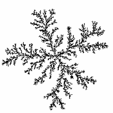
FIG. 1.: A DLA cluster, $n=100000$.

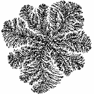
FIG. 2.: A deterministic cluster with a Golden Mean itinerary, $n=100000$.

Other fractal clusters can be obtained by choosing a non-random itinerary [19]. A beautiful family of growth patterns is obtained from quasi-periodic itineraries,

$$\theta_{k+1}=\theta_{k}+2\pi W\ ,$$ (4)

where $W$ is a quadratic irrational number. An example is shown in Fig. 2, in which $W$ is the golden mean $(\sqrt{5}+1)/2$. In [19] it was argued that itineraries obtained from (4) using for $W$ other values of quadratic irrationals lead to clusters of different appearance but the same dimension, which was estimated numerically to be $D=1.86\pm 0.03$. In the same paper other deterministic itineraries (not obtained from circle maps) where shown to lead to clusters with different dimensions. One (trivial) example that is nevertheless useful for our consideration below is the itinerary $\theta_{k}=0$ for all $k$. Such an itinerary grows a 1 dimensional wire of width $\sqrt{\lambda_{0}}$.

The great advantage of the availability of a conformal map is that it affords us analytic power that is not obtainable otherwise. To understand this consider the Laurent expansion of $\Phi^{(n)}(w)$ :

$$\Phi^{(n)}(w)=F^{(n)}_{1}w+F^{(n)}_{0}+F^{(n)}_{-1}w^{-1}+F^{(n)}_{-2}w^{-2}+\dots$$ (5)

The recursion equations for the Laurent coefficients of $\Phi^{(n)}(w)$ can be obtained analytically, and in particular one shows that [16]

$$F_{1}^{(n)}=\prod_{k=1}^{n}[1+\lambda_{k}]^{a}\,.$$ (6)

The first Laurent coefficient $F_{1}^{(n)}$ has a distinguished role in determining the fractal dimension of the cluster, being identical to the Laplace radius which is the radius of a charged disk having the same field far away as the charged cluster [17]. Moreover, defining $R_{n}$ as the minimal radius of all circles in $z$ that contain the $n$-cluster, one can prove that [23]

$$R_{n}\leq 4F_{1}^{(n)}\ .$$ (7)

Accordingly one expects that for sufficiently large clusters (to be made precise below)

$$F^{(n)}_{1}\sim n^{1/D}\sqrt{\lambda_{0}}\ ,\quad n\to\infty\ ,$$ (8)

as $\sqrt{\lambda_{0}}$ remains the only length scale in the problem when the radius of the cluster is much larger than the radius of the initial smooth interface (which we take as the unit circle in this discussion, $\Phi^{(0)}(\omega)=\omega)$).

These observations lead now to the central development of this Letter, and to the most important result. Consider a renormalization process in which we fix the initial smooth interface, but change $\lambda_{0}$, and then rescale $n$ such as to get the “same” cluster. Of course we need to specify what do we mean by the “same” cluster, and a natural requirement is that the electrostatic field on coarse scales (i.e. far from the cluster) will remain invariant. In other words, we should require the invariance of the Laplace radius $F_{1}^{(n)}$ (and possibly of additional low order Laurent coefficients) under renormalization. Clearly, for a given itinerary $\{\theta_{k}\}_{k=1}^{n}$, $F_{1}^{(n)}$ is a function of $n$ and $\lambda_{0}$ only. Accordingly, considering Eq.(8), we note that such a renormalization process can reach a fixed point if and only if $F_{1}^{(n)}(\lambda_{0})$ attains a nontrivial fixed point function $F_{1}^{*}$ of the single “scaling” variable $x=\sqrt{\lambda_{0}}n^{1/D}$. Obviously in the asymptotic limit $x\gg 1$ $F_{1}^{(n)}(\lambda_{0})$ must converge to $F_{1}^{*}$ which is linear in $x$ in this regime. The main new findings of this Letter are that $F_{1}^{*}$ exists as a nonlinear function of $x$, and that $F_{1}^{(n)}(\lambda_{0})$ converges (within every universality class) to its fixed point function $F_{1}^{*}$ already for $x\ll 1$.

In principle one can demonstrate the convergence to $F_{1}^{*}$ analytically. This is easy to do in the case of the degenerate itinerary growing a wire. In this case we can demonstrate convergence after the addition of 2-3 bumps, even in the limit $\lambda_{0}\to 0$, see Fig. 3 . For $x\to 0$ $F_{1}^{*}(x)-1\sim x^{2}$ in this case.

FIG. 3.: The one dimensional wire. We plot $F_{1}(x)-1$ vs. $x=n{\lambda^{1/2}_{0}}$ and demonstrate the convergence to the asymptotic nonlinear function $F_{1}^{*}$. The values of $\lambda_{0}$ used are $10^{-3}$, $10^{-4}$, $10^{-5}$ and $10^{-6}$.

For other nontrivial itineraries it becomes increasingly cumbersome to demonstrate the convergence by hand. With the assistance of the machine we can demonstrate the convergence in all the other cases. In Fig. 4 we present $F_{1}^{(n)}(\lambda_{0})-1$ as a function of $x$ for a typical DLA itinerary and for values of $\lambda_{0}$ ranging between $10^{-8}$ to $10^{-3}$. We note that for $\lambda_{0}\to 0$ the convergence to the fixed point function is obtained infinitesimally close to the initial circle for which $F_{1}^{(n=0)}=1$. In fact, data collapse (with $D$ chosen right) for this itinerary, as well as for all other nontrivial itineraries, is obtained for $n\geq n_{c}$ where $n_{c}\approx 2\pi/\sqrt{\lambda_{0}}$. This is the number of bumps required to obtain one-layer coverage of the original circular interface. Obviously $n^{1/D}_{c}\sqrt{\lambda_{0}}\to 0$ for $\lambda_{0}\to 0$, demonstrating the convergence to $F_{1}^{*}$ for $x\ll 1$. In Fig.5 we exhibit the convergence for the Golden Mean itinerary. Note that the fixed point functions are different, and they both differ from the wire case. The main point of this analysis is that convergence to $F_{1}^{*}$ can be obtained for $x$ arbitrarily small by going to the limit $\lambda_{0}\to 0$.

FIG. 4.: Convergence to $F_{1}^{*}$ for the DLA. We plot $F_{1}(x)-1$ vs. $x=n^{1/D}\lambda^{1/2}_{0}$ with $D=1.7$. The values of $\lambda_{0}$ used are $10^{-3}$ (upper solid line), $10^{-4}$ (upper dashed), $10^{-5}$ (thin solid) $10^{-6}$ (dotted), $10^{-7}$ (lower dashed) and $10^{-8}$ (lower solid). The fixed point function $F_{1}^{*}$ is best approximated by the lowest curve in the figure. Convergence to the asymptotic nonlinear function $F_{1}^{*}$ is seen for smaller $x$ values when $\lambda_{0}$ decreases.

FIG. 5.: Convergence to $F_{1}^{*}$ for the Golden Mean itinerary. Data are same as in Fig. 4 but $x=n^{1/D}\lambda^{1/2}_{0}$ with $D=1.83$. The fixed point function $F_{1}^{*}$ is best approximated by the lowest curve for $x>3\times 10^{-2}$ where the data with $\lambda_{0}=10^{-8}$ converges to $F_{1}^{*}$.

The existence of a fixed point function translates immediately to a calculational scheme. Consider a given itinerary $\{\theta_{k}\}_{k=1}^{N}$ of one of the above classes, and calculate $F_{1}^{(n)}(\lambda_{0})$ for $N>n>n_{c}(\lambda_{0})$. Rescale now $\lambda_{0}\to\lambda_{0}/s$, and calculate $F_{1}^{(n^{\prime})}(\lambda_{0}/s)$ for $N>n^{\prime}>n_{c}(\lambda_{0}/s)$. We can compute $D$ from finding the value $n^{\prime}$ which preserves the Laplace radius under rescaling of $\lambda_{0}$ by $s$:

$$\left(\frac{n^{\prime}}{n}\right)^{1/D}=\sqrt{s}\ .$$ (9)

Since $F_{1}^{*}$ is monotonic (as is immediately seen from Eq.(6)), there is only one solution to this equation,

$$D=\frac{2[\log{n^{\prime}}-\log{n}]}{\log{s}}\ .$$ (10)

As a first example consider the wire case. Computing $F_{1}^{(10)}(10^{-6})$ we find that for $\lambda_{0}=10^{-5}$ the same value of $F_{1}^{(n)}$ is obtained for $n$ between 3 and 4. Eq.(10) with $s=10$ then predicts $0.796<D<1.045$. Repeating for $F_{1}^{(100)}(10^{-6})$ we find the same value of $F_{1}^{(n)}(10^{-5})$ for $n$ between 31 and 32. From Eq.(10) $0.9897<D<1.0173$. We stress that this precision is obtained when $F_{1}^{(n)}-1$ is still 0.0133! Lastly, using $F_{1}^{(500)}(10^{-6})=1.18254$ we compute $0.9951<D<1.0006$, and any desired accuracy can be achieved by increasing $n$. The reader should note that the fractal dimension of the asymptotic cluster ($D=1$ in this case) can be extracted from growth events infinitesimally close to the initial unit circle by decreasing $\lambda_{0}$ (even without increasing $n$ in this specific case). Secondly we consider the deterministic itinerary (4) with Golden Mean winding number. Using values of $F_{1}^{(n)}(10^{-6})$ and $F_{1}^{(n)}(10^{-5})$ between 1.10 and 1.20 we can bound the dimension of the cluster to $1.8305<D<1.8380$. Note that in this case we need to have at least one layer covering which is obtained only when $n_{c}\approx 2\pi/\sqrt{\lambda_{0}}$. Finally, we consider DLA. Here the itineraries are stochastic and one c ould imagine that only under extensive ensemble averaging one would obtain tight bounds on $D$. In fact we find that using values of $F_{1}^{(n)}(10^{-8})$ and $F_{1}^{(n)}(2\times 10^{-8})$ between 1.002 and 1.01 we can bound $D$ as tightly as $1.6896<D<1.7135$. Note that to achieve this accuracy we did not need to go to high values of $F_{1}^{(n)}$, but rather used small values of $\lambda_{0}$ to reach convergence very early. This demonstrates again the unexpected fact that the asymptotic dimension appears as a renormalization exponent right after one or a few layers of particles cover the circle, and very much before $F_{1}^{(n)}\sim n^{1/D}$.

At this point we need to address a few questions:

(i) Why classical numerical estimates [11, 12] of the fractal dimension of DLA converge so slowly?

In standard numerical experiments the radius of gyration of the grown cluster was plotted in log-log coordinates against the number of particles, with $D$ estimated from the slope. Examining our fixed point functions $F_{1}^{*}$ (see Figs.3-5) we note the slow crossover to linear behaviour, which is not fully achieved even for extremely high values of $n$. In this respect we understand from Eq.(7) that a reliable estimate of $D$ from radius of gyration calculation requires inhuman effort, as was indeed experienced by workers in the field [12]. In the present formulation the appearance of the asymptotic $D$ as a renormalization exponent already at early stages of the growth allows a convergent calculation.

(ii) Is a typical DLA cluster self-averaging?

It was demonstrated in [17] that an ensemble of DLA clusters exhibits statistics of $F_{1}^{(n)}$ with standard deviation that shrinks to zero when $n\to\infty$. Nevertheless in [24] it was argued that there may remain residual fluctuations of the dimension $D$ as extracted from (8). The numerics presented above is not sufficient to resolve this question, but additional highly accurate numerics in the limit $\lambda_{0}\to 0,n\to\infty$ should do.

(iii) Is the problem co-dimension 1?

The multi-scaling properties of the harmonic measure have left the impression that computing the fractal dimension of DLA will require a simultaneous control of the host of exponents characterizing the measure. For example the scaling relation $D_{3}=D/2$ (with $D_{3}$ beeing a generalized dimension in the Hentschel-Procaccia sense [21]) that was derived first by Halsey [25] strengthened this impression. The approach presented here indicates that an appropriate fixed point structure can be obtained with only one relevant exponent, i.e. $1/D$, and this exponent appears in the dynamics much before the measure becomes multiscaling.

- [1] T.A. Witten and L.M. Sander, “Diffusion-limited aggregation, a kinetic critical phenomenon”, Phys. Rev. Lett, 47, 1400-1403 (1981).
- [2] L. Niemeyer, L. Pietronero and H.J. Wiessmann, “Fractal dimension of dielectric breakdown” Phys. Rev. Lett. 52, 1033-1036 (1984).
- [3] J. Nittman, G. Daccord and H.E. Stanley, “Fractal growth of viscous fingers: A quantitative characterization of a fluid instability phenomenon”, Nature, 314, 141-144(1985).
- [4] D. Grier, E. Ben-Jacob, R. Clarke, and L.M. Sander, “Morphology and microstructure in electrochemical deposition in zinc”, Phys. Rev. Lett. 56, 1264-1267 (1986).
- [5] R.M. Brady and R.C. Ball, “Fractal growth of copper electrodeposits”, Nature 309, 225-229 (1984);
- [6] J. Kerte’cz and T. Vicsek, “Diffusion-limited aggregation and regular patterns: Fluctuations versus anisotropy”, J. Phys. A 19 L257-L260 (1986).
- [7] G. D’accord and R. Lenormand, “Fractal patterns from chemical dissolution”, Nature 325 41-43 (1987).
- [8] A.D. Fowler, H.E. Stanley and G. D’accord “Disequilibrium silicate mineral textures: Fractal and non-fractal features”, Nature 341, 134-138 (1989).
- [9] E. Ben-Jacob, O. Shochet, A. Tenenbaum, I. Cohen, A. Cziro’k and T. Viscek, “Communicating walkers model for cooperative patterning of bacterial colonies”, Nature 368, 46-49 (1994).
- [10] K.R. Bhaskar, B.S. Turner, P. Garik, J.D. Bradley, R. Bansil, H.E. Stanley and J.T. Lamont, “Viscous fingering of HCl through gastric mucin”, Nature 360, 458-461 (1992).
- [11] P. Meakin “Diffusion-controlled cluster formation in 2-6 dimensional space”, Phys. Rev A 26 1495-1507 (1983).
- [12] B.B. Mandelbrot, “Plane DLA is not self-similar; is it a fractal that becomes increasingly compact as it grows?”, Physica A 191, 95-107 (1992).
- [13] P.Ya. Polubarinova-Kochina, Dokl. Akad. Nauk. SSSR 47, 254 (1945).
- [14] P.G. Saffman and G.I. Taylor, “The penetration of a fluid into a porous medium or Hele-Shaw cell containing a more viscous liquid”, Proc. Roy. Soc. London Series A, 245,312-329 (1958).
- [15] B. Shraiman and D. Bensimon, “Singularities in nonlocal interface dynamics”, Phys.Rev. A30, 2840-2842 (1984).
- [16] M.B. Hastings and L.S. Levitov, “Laplacian growth as one-dimensional turbulence”, Physica D 116, 244-252 (1998).
- [17] B. Davidovitch, H.G.E. Hentschel, Z. Olami, I.Procaccia, L.M. Sander, and E. Somfai, “Diffusion Limited Aggregation and iterated conformal maps”, Phys. Rev. E, 59 1368-1378 (1999).
- [18] B. Davidovitch and I. Procaccia, “Conformal theory of the dimensions of diffusion-limited aggregates”, Euro. Phys. Lett, 48, 547-553 (1999)
- [19] B. Davidovitch, M.J. Feigenbaum, H.G.E. Hentschel and I. Procaccia, “Conformal Theory of Fractal Growth Patterns without Randomness”, Submitted to Phys. Rev. E, also cond-mat/0002420.
- [20] T.C. Halsey, P. Meakin and I. Procaccia, “Scaling structure of the surface layer of diffusion limited aggregates”, Phys. Rev. Lett. 56, 854-857 (1986).
- [21] H.G.E. Hentschel and I. Procaccia, “The infinite number of generalized dimensions of fractals and strange attractors”, Physica D 8, 435-444 (1983).
- [22] T.C. Halsey, M.H. Jensen, L.P. Kadanoff, I. Procaccia and B. Shraiman, “Fractal measures and their singularities: the characterization of strange sets”, Phys. Rev. A, 33, 1141-1151 (1986).
- [23] P.L. Duren, Univalent Functions, (Springer-Verlag, New York, 1983).
- [24] E Somfai, L.M. Sander and R.C. Ball, “Scaling and Crossovers in Diffusion Limited Aggregation”, cond-mat/9909040.
- [25] T.C. Halsey, “Some consequences of an equation of motion for diffuse growth”, Phys. Rev. Lett, 59 2067-2070 (1987).