Ordered phase in the two-dimensional randomly coupled ferromagnet

Abstract

True ground states are evaluated for a $2d$ Ising model with random near neighbor interactions and ferromagnetic second neighbor interactions (the Randomly Coupled Ferromagnet). The spin glass stiffness exponent is positive when the absolute value of the random interaction is weaker than the ferromagnetic interaction. This result demonstrates that in this parameter domain the spin glass like ordering temperature is non-zero for these systems, in strong contrast to the $2d$ Edwards-Anderson spin glass.

75.10.Nr, 75.40.Mg, 02.10.Jf

Introduction

For more than two decades the intensive numerical work on the spin glass (SG) problem has been concentrated almost exclusively on the Edwards-Anderson Ising spin glass : Ising spins on a regular [hyper]cubic lattice with random near neighbor Gaussian or binomial interaction distributions [1]. The many possible alternative Ising systems with a randomness ingredient have hardly been touched on and such results as exist have been largely ignored.

One such family of alternative systems was proposed in [2]. It consists of a 2d square lattice of $L\times L$ Ising spins $\sigma_{i}=\pm 1$ with uniform ferromagnetic second near neighbor interactions of strength $J$, plus random near neighbor interactions $J_{ij}=\pm\lambda J$; we will refer to it as the RCF (Randomly Coupled Ferromagnet) model [3]. It is described by the following Hamiltonian:

$$H=-\sum_{\langle i,j\rangle}J_{ij}\sigma_{i}\sigma_{j}-\sum_{[i,j]}J\sigma_{i}\sigma_{j}\,.$$ (1)

For each realization of the randomness the $J_{ij}$ are drawn with the constraint $\sum_{\langle i,j\rangle}J_{ij}=0$ to reduce fluctuations.

As the spins are coupled through the ferromagnetic second near neighbor interactions, the system can be partitioned into two inter-penetrating sublattices in checkerboard-like fashion. In the limit $\lambda=0$ the two sublattices order ferromagnetically and independently below the Onsager temperature $T=2.27J$. Because each sublattice can order up or down, there are four degenerate ground states. As was pointed out in [2], for non-zero $\lambda$ the near neighbor interactions can be considered in terms of effective random fields exerted by each sublattice on the other, so that for finite $\lambda$ and large enough $L$ the ferromagnetic sublattice ordering is expected to be broken up, as in the $2d$ random field Ising (RFI) model [6]. The ground state will consist of coexisting domains of each of the four types : up/up, up/down, down/up and down/down. The question is: is the break-up accompanied by paramagnetic order down to $T=0$ ?

A number of Monte Carlo simulations were performed, and it was concluded on the basis of standard numerical criteria [2, 3] that when the ratio $\lambda$ is less than about $1$, the RCF systems show spin glass like ordering at a finite temperature, whereas 2d Edwards Anderson ISGs are paramagnetic down to $T=0$ [4]. The finite ordering temperature interpretation was strongly questioned by Parisi et al [5] who criticized the initial work [2] on the grounds that the results were restricted to relatively small sample sizes L. On the basis of Monte Carlo data obtained on rather larger samples Parisi et al suggested that the RCF systems are always paramagnetic down to $T=0$, like the Edwards Anderson ISGs. Further large sample Monte carlo results [3] however indicated finite-temperature ordering.

Here we present data from ground-state configuration evaluations which show unambiguously that RCF systems indeed exhibit finite temperature SG like ordering for $\lambda$ less than about $1$. This opens up new and intriguing possibilities for the testing of fundamental properties of complex ordered systems at finite temperatures in a $2d$ context.

Algorithm

In the present work, ground state configurations have been found for periodic boundary conditions, and for the case where in one direction the boundary conditions are switched to anti-periodic. By comparing the ground state energies of the different boundary conditions for each realization conclusions on the ordering behavior can be obtained. Similar studies were performed for simple $d$-dimensional EA spin glasses in $d=2$ [4], $d=3$ [7], and $d=4$ [8].

For readers not familiar with the calculation of spin-glass ground states now a short introduction to the subject and a description of the algorithm used here are given. A detailed overview can be found in [9]

The concept of frustration [10] is important for understanding the behavior of $\pm J$ Ising spin glasses. The simplest example of a frustrated system is a triple of spins where all pairs are connected by antiferromagnetic bonds, see fig. 1. A bond is called satisfied if it contributes with a negative value to the total energy by choosing the values of its adjacent spins properly. For the triangle it is not possible to find a spin-configuration were all bonds are satisfied. In general a system is frustrated if closed loops of bonds exists, where the product of these bond-values is negative. For square and cubic systems the smallest closed loops consist of four bonds. They are called (elementary) plaquettes.

As we will see later the presence of frustration makes the calculation of exact ground states of such systems computationally hard. Only for the special case of the two-dimensional system with periodic boundary conditions in no more than one direction and without external field a polynomial-time algorithm is known [11]. In general only methods with exponential running times are known, on says the problem is NP-hard [12]. Now for the general case three basic methods are briefly reviewed and the largest system sizes which can be treated are given for three-dimensional systems, the standard spin-glass model, were data for comparison is available.

The simplest method works by enumerating all $2^{N}$ possible states and has obviously an exponential running time. Even a system size of $4^{3}$ is too large. The basic idea of the so called Branch-and-Bound algorithm [13] is to exclude the parts of the state space, where no low-lying states can be found, so that the complete low-energy landscape of systems of size $4^{3}$ can be calculated [14].

A more sophisticated method called Branch-and-Cut [15, 16] works by rewriting the quadratic energy function as a linear function with an additional set of inequalities which must hold for the feasible solutions. Since not all inequalities are known a priori the method iteratively solves the linear problem, looks for inequalities which are violated, and adds them to the set until the solution is found. Since the number of inequalities grows exponentially with the system size the same holds for the computation time of the algorithm. With Branch-and-Cut anyway small systems up to $8^{3}$ are feasible.

The method used here is able to calculate true ground states [7] up to size $14^{3}$. For two-dimensional systems, as considered in this paper, sizes up to $50^{2}$ can be treated. The method is based on a special genetic algorithm [17, 18] and on Cluster-Exact Approximation [19]. CEA is an optimization method designed specially for spin glasses. Its basic idea is to transform the spin glass in a way that graph-theoretical methods can be applied, which work only for systems exhibiting no frustrations. Next a description of the genetic CEA is given.

Genetic algorithms are biologically motivated. An optimal solution is found by treating many instances of the problem in parallel, keeping only better instances and replacing bad ones by new ones (survival of the fittest). The genetic algorithm starts with an initial population of $M_{i}$ randomly initialized spin configurations (= individuals), which are linearly arranged using an array. The last one is also neighbor of the first one. Then $n_{o}\times M_{i}$ times two neighbors from the population are taken (called parents) and two new configurations called offspring are created. For that purpose the triadic crossover is used which turned out to be very efficient for spin glasses: a mask is used which is a third randomly chosen (usually distant) member of the population with a fraction of $0.1$ of its spins reversed. In a first step the offspring are created as copies of the parents. Then those spins are selected, where the orientations of the first parent and the mask agree [20]. The values of these spins are swapped between the two offspring. Then a mutation with a rate of $p_{m}$ is applied to each offspring, i.e. a fraction $p_{m}$ of the spins is reversed.

Next for both offspring the energy is reduced by applying CEA: The method constructs iteratively and randomly a non-frustrated cluster of spins. Spins adjacent to many unsatisfied bonds are more likely to be added to the cluster. During the construction of the cluster a local gauge-transformation of the spin variables is applied so that all interactions between cluster spins become ferromagnetic.

Fig. 2 shows an example of how the construction of the cluster works using a small spin-glass system. For 2d $\pm J$ spin glasses each cluster contains typically 70 percent of all spins. The non-cluster spins act like local magnetic fields on the cluster spins, so the ground state of the cluster is not trivial. Since the cluster has only ferromagnetic interactions, an energetic minimum state for its spins can be calculated in polynomial time by using graph theoretical methods [21, 22]: an equivalent network is constructed [23], the maximum flow [24, 25] is calculated and the spins of the cluster are set to their orientations leading to a minimum in energy. This minimization step is performed $n_{\min}$ times for each offspring.

Afterwards each offspring is compared with one of its parents. The pairs are chosen in the way that the sum of the phenotypic differences between them is minimal. The phenotypic difference is defined here as the number of spins where the two configurations differ. Each parent is replaced if its energy is not lower (i.e. not better) than the corresponding offspring. After this whole step is done $n_{o}\times M_{i}$ times, the population is halved: From each pair of neighbors the configuration which has the higher energy is eliminated. If more than 4 individuals remain the process is continued otherwise it is stopped and the best individual is taken as result of the calculation.

The representation in fig. 3 summarizes the algorithm.

The whole algorithm is performed $n_{R}$ times and all configurations which exhibit the lowest energy are stored, resulting in $n_{g}$ statistical independent ground state configurations. The running time of the algorithm with suitable parameters chosen (see Table I) grows exponentially with the system size. On a 80Mhz PowerPC processor a typical $L=40$ instance takes 3 hours (15 hours for $L=56$).

Results

In this work ground states of the RCF are studied for system sizes up to $L=56$ and values of $\lambda=0.5$, $0.7$, $0.9$, and $1.1$. Usually 1000 different realizations were treated, each submitted to periodic (pbc) and antiperiodic (apbc) boundary conditions in one direction and always pbc in the other direction. The apbc are realized by inverting one line of bonds in the system with pbc. Because of the enormous computational effort, for the largest system sizes only realizations with $\lambda=0.7$ where considered with large statistics (and about 100 realizations with $L=56,\lambda=0.9$).

The periodic ground states give a direct measurement of the $T=0$ break up length $L_{b}$ at each value of $\lambda$, which is defined as follows: For small enough $L$ the ground states will always be such that there is a full ferromagnetic ordering within each sublattice. With increasing $L$, more and more samples will be found with ground states having at least one of the sublattices incompletely ferromagnetic. The break up length $L_{b}$ is defined [26] as the value of $L$ above which more than half the samples do not have pure ferromagnetic order in each sublattice. For the binomial RFI model, $L_{b}\sim 5.5\exp(2/\Delta^{2})$ where $\Delta$ is the strength of the random field [26]. For the RCF the values of $L_{b}$ are shown against $\lambda^{-2}$ in Figure 1. It was suggested in [3] that by analogy with the RFI results [26] $L_{b}(\lambda)$ could be expected to vary as $\exp(1/(4\lambda^{2}))$. In fact the data points for the true ground states lie on the line $L_{b}\sim 3.2\exp(0.62/\lambda^{2})$. For the particular cases $\lambda=0.5$ and $\lambda=0.7$, $L_{b}\approx 45$ and $\approx 10$ respectively. With the wisdom of hindsight, it can be seen that the measurements done in [2, 3, 5] for $\lambda=0.5$ were mainly in the regime $L<L_{b}$ while for $\lambda=0.7$ the larger samples were well in the regime $L>L_{b}$.

A “typical” ground state for $\lambda=0.7$ and $L=56$ is shown in Figure 5. All four possible types of domains occur. Because of the discrete structure of the interaction usually the ground state is degenerate. But in contrast to the EA spin glasses with only $\pm J$ near neighbor interactions, where a complex ground-state landscape exists, the structure of the degeneracy is trivial for $\lambda\leq 1$: the whole system may be flipped, sometimes it is possible to flip both sublattices independently, and usually some small clusters occur with can take two orientations.

But for studying whether the model exhibits long range order or not, it is sufficient to concentrate on the ground-state energies $E_{P},E_{AP}$ for periodic and antiperiodic boundary conditions. The energy differences $\Delta=E_{P}-E_{AP}$ give information about whether a system exhibits some kind of stiffness against perturbations of the boundary, i.e. about the presence of order. $\Delta$ is called the stiffness energy. For samples with the same set of interactions the stiffness can be analyzed in terms of the size dependence of the average $\langle\Delta\rangle$ and of the width $W\equiv\sqrt{\sigma^{2}(\Delta)}$ of the distribution $P(\Delta)$. For $\lambda=0.7$ the distribution is presented in Fig. 6. The inset shows the behavior of the average stiffness energy as a function of $L$ for all four values of $\lambda$. For system sizes larger the breakup length and $\lambda\geq 0.7$ the stiffness energy decreases, indicating that no ferromagnetic long range order is present in the system. For $\lambda=0.5$ the breakup length is very large, so the asymptotic behavior is hardly visible, but $\langle\Delta\rangle$ seems to fall for $L\geq 28$. From direct evaluation of the magnetization (see Fig 7 and Fig. 8) we conclude that no ferromagnetic order should be present beyond an upper limit $\lambda=0.27(8)$. For smaller values of $\lambda$ nothing can be concluded from our data. Furthermore, for smaller values of $\lambda$ it remains possible that the ground states of the RCF model do not exhibit ferromagnetic ordering ordering for any finite value of the relative coupling constant $\lambda$.

From standard relationships [27, 28] one can write $\langle\Delta\rangle\sim L^{\theta_{F}}$ with $\theta_{F}$ the ferromagnetic stiffness exponent, and $W\sim L^{\theta_{SG}}$ with $\theta_{SG}$ the spin glass stiffness exponent. Positive values of the exponents indicate a long range order. Because of the small system sizes an evaluation of the ferromagnetic exponent is difficult. From the results presented in Fig. 6 we find an asymptotic ($L\to\infty$) value of $\theta_{F}=-2$ ($\lambda=0.9,1.1$).

Now we turn to the question whether some kind of spin-glass order is present in the system. This can be investigated by analyzing The dependence of the variance $\sigma^{2}(\Delta)$ of the stiffness-energy distributions on the system size, the result is shown in Fig. 9. For small system sizes the variance grows for all values of the coupling constant $\lambda$. In order to exclude finite-size effects, only systems larger than the breakup length $L_{b}(\lambda)$ should be taken into account. Above $L_{b}$ there is a good linear size dependence of $\log W(L)$ against $\log L$, with $\theta_{SG}=0.59(8)$, $0.29(1)$, $0.09(5)$, and $-0.16(2)$ respectively for $\lambda=0.5,0.7,0.9$, and $1.1$.

The values of $\theta_{SG}$ against $\lambda$ are shown in the inset of Figure 9. The result for $\lambda=0.5$ is not very reliable, because the largest system size is of the order of the breakup length. In the log-log plot the datapoints for $\lambda=0.5$ exhibit a negative curvature, thus the asymptotic value of $\theta_{SG}$ may be smaller than $0.59$. For the other systems the breakup length is quite small, so the results give unambiguous evidence for spin glass like ordering in the large size limit, with a non-zero ordering temperature. Especially for $\lambda=0.7$, where $L_{b}\approx 10$, the result $\sigma(\Delta)>0$ is very reliable. Thus, it is indeed not necessary to carry out further calculations with larger systems to prove the fact, there there are values of the coupling constant giving rise to an ordered spin glass phase in the RCF. The limiting value $\lambda_{c}$ above which $\theta_{SG}$ is negative is very close to $1.0$; $\lambda_{c}$ would correspond to the highest value at which the ordering temperature is non-zero, in good agreement with the initial estimate from the Monte Carlo work [2].

Conclusion

We have calculated ground states of the Randomly Coupled Ferromagnet for different values of the spin-glass coupling constant $\lambda$ and with periodic as well as antiperiodic boundary conditions. By using the genetic cluster-exact approximation algorithm, we were able to treat system sizes up to $N=56\times 56$. The breakup length was calculated for each value of $\lambda$. From the calculation of $T=0$ stiffness energy it could be concluded that below $\lambda_{c}\approx 1$ the RCF exhibits an ordered spin glass like phase at finite temperature. It should be stressed again that for $\lambda>0.5$ the largest system sizes are well beyond the breakup length, so no changes are to be expected for larger system sizes. For $\lambda<0.5$, especially if one likes to test whether the model exhibits ferromagnetic ordering, ground states calculations of larger systems are needed to study the behavior in more detail. Unfortunatley, these studies are beyond the power of current computers and algorithms.

Although the zero-temperature stiffness exponent values give no direct information on the ordering temperatures, the present results are consistent with the the conclusions drawn in [2, 3] where Monte Carlo estimates of the critical temperatures were made using the finite-size scaling of the spin glass susceptibility and the form of the time dependence of the autocorrelation function relaxation. Ordering temperatures were estimated to be close to $2.0$ for $\lambda=0.5$ and $0.7$, dropping to zero near $\lambda=1$. Rather remarkably the $T=0$ crossover as a function of $L$ at $L_{b}$ appears to have little effect on the behavior of the SG susceptibility as a function of size in the temperature region close to $T_{g}$ [3]. However for $\lambda=0.5$ Parisi et al [5] observed weakly non-monotonic behavior of the Binder parameter with $L$ for sizes that we now know to be in the region of the crossover.

Since the existence of a spin glass like phase at finite temperature now has been established definitely, it would be instructive to carry out further careful Monte Carlo measurements for sample sizes well in the regime $L>L_{b}$ and over a range of $\lambda$ values. Is the physics of the $2d$ RCF above, at, and below the ordering temperature strictly analogous to that of the standard Edwards Anderson ISG at dimensions where there is finite temperature ordering? To what extent could the RCF enlighten us concerning problems which in the Edwards Anderson ISG context have remained conflictual for more than twenty years ? The fact that the RCF lives on a $2d$ lattice rather than in a higher dimension should facilitate understanding of the fundamental physics of ordering in complex systems.

Finally, there may even be possible experimental realizations of systems where quasi-two-dimensional magnets form short range clusters with local ferromagnetic or antiferromagnetic order, with random frustrated interactions linking these clusters together. Examples of promising behaviour of this sort are Fe compound with halogens [29] where it might be interesting to look at the data again in view of the present results.

$L$	$M_{i}$	$n_{o}$	$n_{\min}$	$p_{m}$	$n_{R}$
5	8	1	1	0.05	5
10	16	1	2	0.05	5
14	16	2	2	0.05	5
20	32	8	2	0.05	5
28	128	16	2	0.05	5
40	512	16	2	0.05	5
56	1024	16	2	0.05	5

TABLE I.: Simulation parameters: $L$ = system size, $M_{i}$ = initial size of population, $\nu$ = average number of offsprings per configuration, $n_{\min}$ = number of CEA minimization steps per offspring, $p_{m}$ = mutation rate, $n_{R}$=number of independent runs per realization.

FIG. 1.: The simplest frustrated system: a triple of spins, each pair of spins connected by antiferromagnetic bonds (dashed lines). It is not possible to satisfy all bonds.

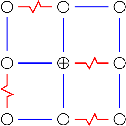
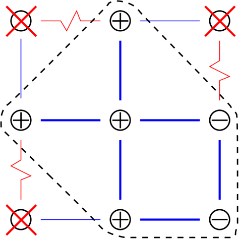
FIG. 2.: Example of the Cluster-Exact Approximation method. A part of a spin glass is shown. The circles represent lattice sites/spins. Straight lines represent ferromagnetic bonds the jagged lines antiferromagnetic interactions. The top part shows the initial situation. The construction starts with the spin at the center. The bottom part displays the final stage. The spins which belong to the cluster carry a plus or minus sign which indicates how each spin is transformed, so that only ferromagnetic interactions remain inside the cluster. All other spins cannot be added to the cluster because it is not possible to multiply them by $\pm 1$ to make all adjacent bonds positive. Please note that many other combinations of spins can be used to build a cluster without frustration.

algorithm genetic CEA($\{J_{ij}\}$, $M_{i}$, $n_{o}$, $p_{m}$, $n_{\min}$)
begin
	create $M_{i}$ configurations randomly
	while ($M_{i}>4$) do
	begin
		for $i=1$ to $n_{o}\times M_{i}$ do
		begin
			select two neighbors
			create two offspring using triadic crossover
			do mutations with rate $p_{m}$
			for both offspring do
			begin
				for $j=1$ to $n_{\min}$ do
				begin
					construct unfrustrated cluster of spins
					construct equivalent network
					calculate maximum flow
					construct minimum cut
					set new orientations of cluster spins
				end
				if offspring is not worse than related parent
				then
					replace parent with offspring
			end
		end
		half population; $M_{i}=M_{i}/2$
	end
	return one configuration with lowest energy
end

FIG. 3.: Genetic Cluster-exact Approximation.

FIG. 4.: Breakup length $L_{b}$ as a function of $1/\lambda^{2}$. The solid line shows a fit to the function $L_{b}(\lambda)=a\exp(-b/\lambda^{2})$.

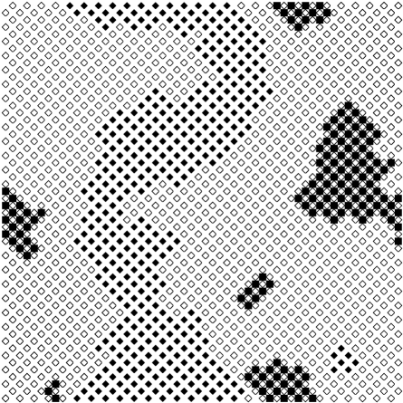
FIG. 5.: Typical ground state of one RCF realization ($L=56$) for $\lambda=0.70$ with periodic boundary conditions in all directions. Two different symbols (white/black square), (unfilled/filled diamond) are used to represent the orientations on the different sublattices.

FIG. 6.: Distribution of stiffness energies $\Delta$ at $\lambda=0.7$ for different system sizes $L=14,28,56$. The inset shows the mean stiffness energy $\langle\Delta\rangle$ as a function of $L$ for $\lambda=0.5$, $0.7$, $0.9$, and $1.1$.

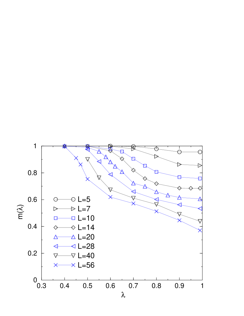
FIG. 7.: Average magnetization $m$ as a function of the strength $\lambda$ of the spin-glass couplings for different systems sizes $5\leq L\leq 56$.

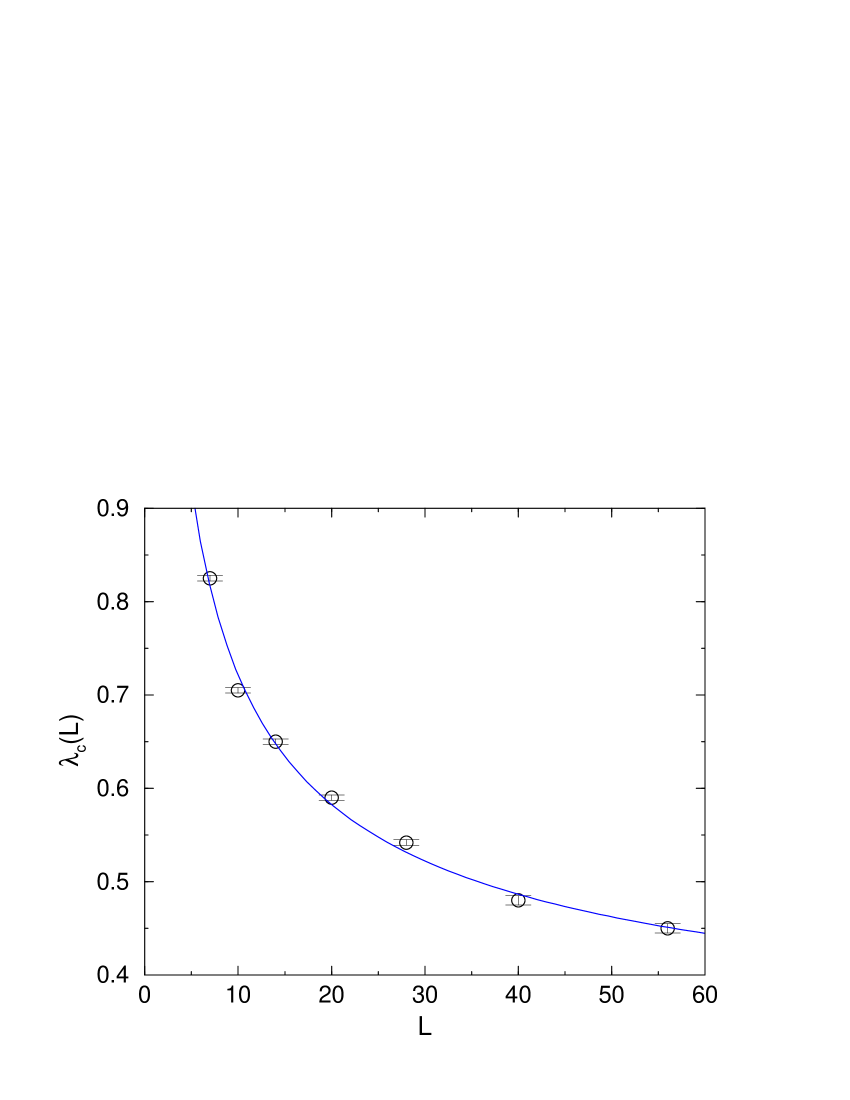
FIG. 8.: Threshold value $\lambda_{c}$ as a function of the system size $L$. The threshold value is determined from $m(\lambda_{c})=0.9$. The solid line shows a fit to a function $\lambda_{c}(L)=\lambda_{\infty}+eL^{-f}$, resulting in $\lambda_{\infty}=0.27(8)$, $f=-0.53(10)$.

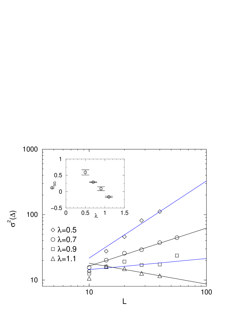
FIG. 9.: Width $\sigma^{2}(\Delta)$ of the distribution of stiffness energies as a function of the system size $L\geq 10$ for $\lambda=0.5,0.7,0.9,1.1$. The solid lines are fits to algebraic functions of the form $\sigma^{2}(L)=gL^{\theta_{SG}}$. The inset shows the values of the exponent for different values of $\lambda$.

REFERENCES

- [1] For reviews on spin glasses see: K. Binder and A.P. Young, Rev. Mod. Phys. 58, 801 (1986); M. Mezard, G. Parisi, M.A. Virasoro, Spin glass theory and beyond, World Scientific, Singapore 1987; K.H. Fisher and J.A. Hertz, Spin Glasses, Cambridge University Press, 1991
- [2] N. Lemke and I.A. Campbell, Phys. Rev. Lett. 76, 4616 (1996)
- [3] N. Lemke and I.A. Campbell, J. Phys.A 32, 7851 (1999)
- [4] N. Kawashima and H. Rieger, Europhys. Lett. 39, 85 (1997)
- [5] G. Parisi, J.J. Luiz-lorenzo, and D.A. Stariolo, J. Phys A 31 4657, (1998)
- [6] Y. Imry and S.-K. Ma, Phys. Rev. Lett. 35, 1399 (1975), M. Aizenman and J. Wehr, Phys. Rev. Lett. 62, 2503 (1989)
- [7] A.K. Hartmann, Phys. Rev. E 59, 84 (1999)
- [8] A.K. Hartmann, Phys. Rev. E 60, 5135 (1999)
- [9] H. Rieger, in: Advances in Computer Simulation, ed. J. Kertesz and I. Kondor, Lecture Notes in Physics 501, (Springer-Verlag, Heidelberg, 1998)
- [10] G. Toulouse, Commun. Phys. 2, 115 (1977)
- [11] F. Barahona, R. Maynard, R. Rammal and J.P. Uhry, J. Phys. A 15, 673 (1982).
- [12] F. Barahona, J. Phys. A 15, 3241 (1982)
- [13] A. Hartwig, F. Daske and S. Kobe, Comp. Phys. Commun. 32 133 (1984)
- [14] T. Klotz and S. Kobe, J. Phys. A: Math. Gen. 27, L95 (1994)
- [15] C. De Simone, M. Diehl, M. Jünger, P. Mutzel, G. Reinelt and G. Rinaldi, J. Stat. Phys. 80, 487 (1995)
- [16] C. De Simone, M. Diehl, M. Jünger, P. Mutzel, G. Reinelt and G. Rinaldi, J. Stat. Phys. 84, 1363 (1996)
- [17] K.F. Pál, Physica A 223, 283 (1996)
- [18] Z. Michalewicz, Genetic Algorithms + Data Structures = Evolution Programs, Springer, Berlin 1992
- [19] A.K. Hartmann, Physica A 224, 480 (1996)
- [20] K.F. Pál, Biol. Cybern. 73, 335 (1995)
- [21] J.D. Claiborne, Mathematical Preliminaries for Computer Networking, Wiley, New York 1990
- [22] M.N.S. Swamy and K. Thulasiraman, Graphs, Networks and Algorithms, Wiley, New York 1991
- [23] J.-C. Picard and H.D. Ratliff, Networks 5, 357 (1975)
- [24] J.L. Träff, Eur. J. Oper. Res. 89, 564 (1996)
- [25] R.E. Tarjan, Data Structures and Network Algorithms, Society for industrial and applied mathematics, Philadelphia 1983
- [26] E.T. Seppälä, V. Petäjä and M.J. Alava, Phys.Rev.E 58 5217, (1998)
- [27] A.J. Bray and M.A. Moore, J. Phys. C 17, L463 (1984)
- [28] W.L. McMillan, Phys. Rev. B 30, 476 (1984)
- [29] J. Vetel, M. Yahiaoui, D. Bertrand, A.R. Fert, J.P. Redoules and J. Ferre J. Physique, Colloque C8, 49 1067 (1988), D. Bertrand, F. Bensamka, A.R. Fert, J. Gelard, J.P. Redoules and S. Legrand J. Phys. C: Solid State Phys. 17 1725 (1984)