Mean parameter model for the Pekar-Fröhlich polaron
in a multilayered heterostructure

Abstract

The polaron energy and the effective mass are calculated for an electron confined in a finite quantum well constructed of $GaAs/Al_{x}Ga_{1-x}As$ layers. To simplify the study we suggest a model in which parameters of a medium are averaged over the ground-state wave function. The rectangular and the Rosen-Morse potential are used as examples.

To describe the confined electron properties explicitly to the second order of perturbations in powers of the electron-phonon coupling constant we use the exact energy-dependent Green function for the Rosen-Morse confining potential. In the case of the rectangular potential, the sum over all intermediate virtual states is calculated. The comparison is made with the often used leading term approximation when only the ground-state is taken into account as a virtual state. It is shown that the results are quite different, so the incorporation of all virtual states and especially those of the continuous spectrum is essential.

Our model reproduces the correct three-dimensional asymptotics at both small and large widths. We obtained a rather monotonous behavior of the polaron energy as a function of the confining potential width and found a peak of the effective mass. The comparison is made with theoretical results by other authors. We found that our model gives practically the same (or very close) results as the explicit calculations for potential widths $L\geq 10\AA$.

I Introduction

Quasi-two-dimensional (2D) systems have attracted a lot of attention during the last decade because of their practical realization. If a heterostructure is made of polar materials such as $GaAs$, $InAs$ etc., the electron-phonon interaction modifies the properties of the electron confined to a 2D-structure resulting in a shift of the binding energy and the effective band mass.

The polaron effects in a 2D electron gas have extensively been studied. At earlier stages the attention was paid to the properties of a polaron confined to an infinite thin 2D layer[3, 4, 5]. The binding energy and the effective mass were calculated for a $GaAs/Al_{x}Ga_{1-x}As$ infinitely deep quantum well of a finite length[6, 7]. In these papers only the interaction with the bulk LO-phonon mode has been taken into account. Actually, LO-phonon modes are modified in a 2D layer (the so-called confined slab LO-phonon modes). Besides, there exist interface optical-phonon modes as well as half-space LO-phonon modes in a barrier material[8, 9, 10, 11, 12]. For the review of these modes (also in complicated multi-layer structures) see the book by Pokatilov, Fomin and Beril[13] and also more recent publications [14, 15] of this group. The influence of the mentioned modes on polarons were studied in Refs. [16, 17, 18, 19].

While different phonon modes were studied in details, the quantum well potential was supposed to be infinitely deep in the cited papers. On the other hand, the properties of the system would be quite different if a confining potential had a finite depth. Indeed, for an infinitely deep confining potential the binding energy is the monotonous function of the potential width which varies between limiting values $E^{(in)}_{3D}=\alpha_{in}\hbar\omega_{in}$ for the three-dimensional (3D) space and $E^{(in)}_{2D}=(\pi/2)\,\alpha_{in}\hbar\omega_{in}$, where $\alpha_{in}$ is the standard Fröhlich electron-phonon coupling constant and $\omega_{in}$ is the LO-phonons frequency for the quantum well material. If a particle is confined to a finite potential well, the limiting value of the binding energy should be the same at large width of the well. But when the width becomes too small, the energy level approaches the edge of the well, so that effectively the particle is spread over the 3D space. Thus, the limiting value of the binding energy should coincide with the 3D limiting value rather than with the 2D one. This means, the binding energy takes the value $E^{(out)}_{3D}=\alpha_{out}\hbar\omega_{out}$ at small widths where the parameters $\omega_{out}$ and $\alpha_{out}$ are now related to the barrier material. The binding energy evidently has a peak at some intermediate value of the width if $E^{(out)}_{3D}\leq E^{(in)}_{3D}$. If this is not the case, the existence of the peak should be checked in more detail.

Different rectangular quantum wells of a finite height have been investigated by Hai, Peeters and Devreese[20, 21] and Shi, Zhu et al.[22] in the scope of the second order perturbation theory in powers of the electron-phonon coupling constant $\alpha$ with all phonon modes being incorporated. Peaks of the phonon induced energy shift and the polaron effective mass were found for some values of the confining potential widths.

In principle, the same approach can be used while dealing with a quantum well constructed of layers of different materials. But the problem becomes then too complicated because one has to take into account interface phonon modes at each frontier of different materials as well as quantized phonon modes inside each of the layers. The main goal of the present paper is to formulate a simplified model to take these effects into account and to deal with the effective confining potential and only one bulk phonon mode. We calculate polaron characteristics for the same rectangular quantum well as in Refs. [20, 21, 22] to compare the results. Another example is given of a quantum well of the finite depth for which the second-order correction due to the electron-phonon interaction can be calculated explicitly. Namely, we take the Rosen-Morse potential to confine electrons to a 2D-multilayered heterostructure and calculate the shift of the ground-state energy and the effective mass perturbatively, that is, in the weak-coupling limit. In contrast with the rectangular potential we should not worry about the correct including of all virtual states because the Green function is known analytically for this system.

II Formulation of the model

Let us consider a quantum well in the $z$ direction constructed of the $xy$ plane layers of $GaAs/Al_{x}Ga_{1-x}As$. That is, the $AlAs$ mole fraction $x$ depends on the coordinate $z$: $x=x(z)$. The energy gap between different materials forms the confining potential $V(z)$ which serves us as the main entity. Given the potential $V(z)$, one can find the corresponding mole fractions $x(z)$ and a dependence on $z$ of any of the medium parameters (such as the electron band mass $m(z)$, phonon frequencies $\omega(z)$, dielectric constants $\varepsilon_{0}(z),\varepsilon_{\infty}(z)$, Fröhlich coupling constants $\alpha(z)$, etc.).

To avoid difficulties with mass mismatch in different layers we suggest to use a mean band mass $m$ which is common for all layers. Then we start with the following expression for the electronic part of the Hamiltonian:

$$H_{el} = H_{el,\parallel}+H_{el,\perp},$$ (1)

$$H_{el,\parallel} = {\vec{p}_{\parallel}^{\,2}\over 2m},\quad H_{el,\perp}={p_{z}^{\,2}\over 2m}+V(z),$$ (2)

where the electron mean band mass is defined by the relation

$${1\over m}=\int dz\,{|\psi_{1}(z)|^{2}\over m(z)}$$ (3)

and the ground state wave function $\psi_{1}(z)$ for the electron motion in $z$ direction is a solution to the Schrödinger equation

$$H_{el,\perp}\psi_{1}=E_{1}\psi_{1}$$ (4)

with $E_{1}$ being a ground state energy. As the wave function $\psi_{1}$ also depends on the mean band mass $m$, the latter can be found as a self-consistent solution of Eqs. (3), (4).

In a similar way we define the free LO-phonon Hamiltonian

$$H_{ph}=\hbar\omega_{\mbox{LO}}\sum\limits_{\vec{k}}a^{{\dagger}}_{\vec{k}}a_{\vec{k}},$$ (5)

where $a^{{\dagger}}_{\vec{k}}\;(a_{\vec{k}})$ are creation (annihilation) operators of a phonon with a wave vector $\vec{k}$, and mean frequency $\omega_{\mbox{LO}}$ can be found from the expression

$$\omega_{\mbox{LO}}=\int dz\,\omega(z)\,|\psi_{1}(z)|^{2}.$$ (6)

Evidently, we have to address why the free phonon Hamiltonian is averaged with respect to the electron wave function. Our motivation is based on the fact that we are going to apply our model to calculate polaron effects. That is, our effective phonons will be considered only in a cloud around the electron, and the properties of this cloud depend on the electron position. So, in our model the effective phonons replace numerous phonon modes whose frequencies depend on the coordinate $z$ of the electron.

Finally, we accept the conventional form of the Hamiltonian describing the interaction of the electron with effective phonons:

$$H_{int}=\sum_{\vec{k}}\,\left(a_{\vec{k}}\,V_{\vec{k}}\,e^{i\vec{k}\cdot\vec{r}}+a^{{\dagger}}_{\vec{k}}\,V^{*}_{\vec{k}}\,e^{-i\vec{k}\cdot\vec{r}}\right),$$ (7)

where the Fourier transforms of the electron-phonon interaction potential are specified as follows:

$$V_{\vec{k}}=-i\hbar\omega_{\mbox{LO}}\left({4\pi\alpha\over Vk^{2}}\sqrt{{\hbar\over 2m\omega_{\mbox{LO}}}}\right)^{1/2}.$$ (8)

Here the use is made of a mean Fröhlich coupling constant $\alpha$ which can be found from the relation

$$\sqrt{\alpha}=\int dz\,|\psi_{1}(z)|^{2}\,{\omega(z)\over\omega_{\mbox{LO}}}\left(\alpha(z)\sqrt{m\omega_{\mbox{LO}}\over m(z)\omega(z)}\right)^{1/2}.$$ (9)

Note that we define the mean parameters in Eqs. (3), (6), (9) according to the way they enter the Hamiltonian.

Thus, we describe a complicated multilayered heterostructure by the Hamiltonian

$$H=H_{el}+H_{ph}+H_{int}$$ (10)

with the bulk phonon mode only which inhabits an effective medium with mean characteristics defined above. The details of the heterostructure are taken into account by the confining potential $V(z)$.

Performing a unitary transformation $H\to H^{\prime}=U^{-1}HU$ with the operator

$$U=\exp\left[-i\vec{r}_{\parallel}\sum_{\vec{k}}\vec{k}_{\parallel}a^{{\dagger}}_{\vec{k}}a_{\vec{k}}\right],$$ (11)

we arrive at the Hamiltonian

$$H^{\prime}=H^{\prime}_{el,\parallel}+H_{el,\perp}+H_{ph}+H^{\prime}_{int},$$ (13)

$$H^{\prime}_{el,\parallel} = {1\over 2m}\left(\vec{p}_{\parallel}-\hbar\sum_{\vec{k}}\vec{k}_{\parallel}a^{{\dagger}}_{\vec{k}}a_{\vec{k}}\right)^{2},$$ (14)

$$H^{\prime}_{int}=\sum_{\vec{k}}\,\left(a_{\vec{k}}\,V_{\vec{k}}\,e^{ik_{z}\cdot z}+a^{{\dagger}}_{\vec{k}}\,V^{*}_{\vec{k}}\,e^{-ik_{z}\cdot z}\right).$$ (15)

The quantity $\vec{p}_{\parallel}$ is a c-number corresponding to the conserved momentum in the $xy$ plane and the Hamiltonians $H_{el,\perp},H_{ph}$ are defined by Eqs. (2), (5), respectively.

Keeping in mind the smallness of the electron-phonon coupling constant $\alpha$ for most of the materials, we calculate the second-order correction to the unperturbed Hamiltonian $H^{\prime}_{0}=H^{\prime}_{el,\parallel}+H_{el,\perp}+H_{ph}$ (note that the quantum-mechanical first-order correction is equal to zero). The unperturbed energy levels are given by the expression

$$E(\vec{p}_{\parallel},n_{\vec{k}},N) = {1\over 2m}\left(\vec{p}_{\parallel}-\hbar\sum_{\vec{k}}\vec{k}_{\parallel}n_{\vec{k}}\right)^{2}+$$ (17)

$$\hbar\omega_{\mbox{LO}}\sum_{\vec{k}}\,n_{\vec{k}}+E_{N},$$

where $n_{\vec{k}}$ is the number of phonons with the wave vector $\vec{k}$. The energy $E_{N}$ is the $N$-th energy level of the one-dimensional system $H_{el,\perp}$ of Eq. (2). Here $N$ is the corresponding quantum number not necessarily a discrete one: it stands for both the quantum number $n$ which varies from 1 to $n_{max}$ and the wave vector $q$ of the continuous spectrum states.

The wave functions of the unperturbed Hamiltonian $H^{\prime}_{0}$ are given by the direct product

$$|\vec{p}_{\parallel};n_{\vec{k}},N\rangle=|n_{\vec{k}}\rangle\otimes|N\rangle$$ (18)

of the corresponding wave functions of different terms in $H^{\prime}_{0}$.

Because of the structure of the interaction term $H^{\prime}_{int}$ only intermediate states with one phonon contribute to the second order correction to the ground-state energy. The latter is then given by the expression

$$\Delta_{2}E(\vec{p}_{\parallel})=$$ (19)

$$-\sum\limits_{N,\vec{k}}{|V_{\vec{k}}|^{2}\ |G(N,k_{z})|^{2}\over E_{N}+\hbar\omega_{\mbox{LO}}+\displaystyle{(\vec{p}_{\parallel}-\hbar\vec{k}_{\parallel})^{2}-{\vec{p}_{\parallel}}^{\,2}\over 2m}-E_{1}},$$ (20)

where

$$G(N,k_{z})=\int\limits_{-\infty}^{\infty}dz\,\psi_{N}(z)\psi_{1}(z)e^{ik_{z}z}$$ (21)

and $\psi_{N}(z)$ are the wave functions of the Hamiltonian $H_{el,\perp}$ in Eq. (2). The concrete application of these formulae is given in the following section.

III Rectangular Potential

A Medium mean characteristics

As an example we now consider the rectangular confining potential

$$V(z)=\left\{\begin{array}[]{ll}0,&|z|\leq L/2\\ V_{0},&|z|>L/2\end{array}\right.$$ (24)

and

$$m(z)=\left\{\begin{array}[]{ll}m_{in},&|z|\leq L/2\\ m_{out},&|z|>L/2\end{array}\right.$$ (27)

with $m_{in}\ (m_{out})$ being the electron band masses in the well (barrier) material, respectively. For concreteness we assume $GaAs$ to be the quantum well material and $Al_{x}Ga_{1-x}As$ to be the barrier material.

Symmetrical wave functions of the discrete spectrum in the rectangular quantum well with the mean band mass $m$ take the form

$$\psi_{s,n}=N_{s,n}\left\{\begin{array}[]{ll}\cos q_{n}z,&|z|\leq L/2\\ \cos\displaystyle{q_{n}L\over 2}e^{-p_{n}(|z|-L/2)},&|z|>L/2,\end{array}\right.$$ (30)

where

$$p_{n}=\sqrt{q_{max}^{2}-q_{n}^{2}},\quad q_{max}^{2}={2mV_{0}\over\hbar^{2}}$$ (31)

and the normalization constant is given by

$$N_{s,n}=\sqrt{2p_{n}\over p_{n}L+2}.$$ (32)

Antisymmetrical wave functions of the discrete spectrum take the form

$$\psi_{a,n}=N_{s,n}\left\{\begin{array}[]{ll}\sin q_{n}z,&|z|\leq L/2\\ \mbox{\rm sgn}(z)\,\sin\displaystyle{q_{n}L\over 2}e^{-p_{n}(|z|-L/2)},&|z|>L/2\end{array}\right.$$ (35)

(36)

with the same normalization constant given by Eq. (32).

The total number $n_{max}$ of the discrete energy levels is given by the expression

$$n_{max}=1+\left[{q_{max}L\over\pi}\right],$$ (37)

where $[A]$ is an integer part of a number $A$. The expression for the discrete energy levels reads as follows:

$${q_{n}L\over 2}=\mbox{\rm atan}\,\sqrt{{q_{max}^{2}\over q_{n}^{2}}-1}+{\pi(n-1)\over 2},\quad n=1,2,\ldots.$$ (38)

Energies with odd (even) $n$ correspond to the symmetrical (antisymmetrical) wave functions.

The energy $E_{q}=\hbar^{2}q^{2}/2m$ of the continuous spectrum state depends on the wave vector $q$. The corresponding symmetrical wave functions are as follows:

$$\psi_{s,q}={N_{s,q}\over\sqrt{L_{z}}}\left\{\begin{array}[]{ll}p\cos qz,&|z|\leq L/2,\\[14.22636pt] p\cos\displaystyle{qL\over 2}\cos\displaystyle p(|z|-L/2)-\\[5.69054pt] q\sin\displaystyle{qL\over 2}\sin p(|z|-L/2),&|z|>L/2,\\ \end{array}\right.$$ (42)

(43)

where

$$p=\sqrt{q^{2}-q^{2}_{max}}$$ (44)

and $L_{z}$ is the (infinite) size of the system in the $z$ direction. The normalization constant is given by the expression

$$N_{s,q}=\sqrt{2\over p^{2}\cos^{2}\displaystyle{qL\over 2}+q^{2}\sin^{2}\displaystyle{qL\over 2}}.$$ (45)

The antisymmetrical wave functions are as follows:

$$\psi_{a,q}={N_{a,q}\ \mbox{\rm sgn}(z)\over\sqrt{L_{z}}}\left\{\begin{array}[]{ll}p\sin q|z|,\quad|z|\leq L/2,\\[14.22636pt] p\sin\displaystyle{qL\over 2}\cos p(|z|-L/2)+\\[5.69054pt] q\cos\displaystyle{qL\over 2}\sin p(|z|-L/2),\\ \qquad\qquad\qquad|z|>L/2,\end{array}\right.$$ (50)

(51)

where the normalization constant is given by the expression

$$N_{a,q}=\sqrt{2\over p^{2}\sin^{2}\displaystyle{qL\over 2}+q^{2}\cos^{2}\displaystyle{qL\over 2}}.$$ (52)

The electron mean band mass is defined as

$${1\over m} = {W_{in}\over m_{in}}+{W_{out}\over m_{out}}\rightarrow$$ (53)

$$m = {m_{in}m_{out}\over W_{in}m_{out}+(1-W_{in})m_{in}},$$ (54)

where $W_{in}$ and $W_{out}=1-W_{in}$ are probabilities to find the electron inside (outside) the quantum well. The expression for $W_{in}$ follows from Eq. (30)

$$W_{in}=2N^{2}_{s,1}\int\limits_{0}^{L/2}dz\,\cos^{2}q_{1}z=1-{(q_{1}/q_{max})^{2}\over 1+p_{1}L/2},$$ (55)

where $q_{1}$ is a solution to Eq. (38) for the ground-state ($n=1$).

To finish this subsection, we note that the exact energy levels in the rectangular potential with different masses $m_{in}$ and $m_{out}$ calculated for the $GaAs/Al_{x}Ga_{1-x}As$ heterostructure practically coincide with the levels obtained with the electron mean band mass $m$. To obtain an inner criterion of the validity of the anzatz concerning the mean band mass we notice that the particle being on lowest energy levels is located mostly inside the well which means that its band mass is almost coincide with $m_{in}$.

One can await the largest discrepancy for a level near the potential edge. The $n$-th discrete level appears at the width $L=L^{(av)}_{n}$, where

$$L^{(av)}_{n}=\pi(n-1){\hbar\over\sqrt{2mV_{0}}}={\pi(n-1)\over q_{\max}},$$ (56)

and the analogous width for the exact solution reads as follows:

$$L^{(ex)}_{n}=\pi(n-1){\hbar\over\sqrt{2m_{in}V_{0}}}.$$ (57)

Thus, the ratio

$${L^{(av)}_{n}\over L^{(ex)}_{n}}=\sqrt{m_{in}\over m}=\sqrt{W_{in}+(1-W_{in}){m_{in}\over m_{out}}}.$$ (58)

can serve us as the numerical criterion of the validity of the anzatz. The largest discrepancy happens at $n=2$ and in this case Eqs. (31), (38) (55) lead to the following expression:

$${L^{(av)}\over L^{(ex)}}=\sqrt{0.844+0.156{m_{in}\over m_{out}}}.$$ (59)

Note that numerical coefficients here do not depend on the material parameters. For the $GaAs/Al_{0.3}Ga_{0.7}As$ quantum well we have $m_{in}/m_{out}\approx 0.7$ and the discrepancy is about $2\%$; in the worst possible case when $m_{in}/m_{out}\ll 1$ the discrepancy is still not large: $100\%\sqrt{0.844}\approx 8\%$.

B Electron-phonon correction to the polaron energy and the effective mass

Summation over the wave vector $\vec{k}$ in Eq. (20) can be reduced to integration in a conventional way

$$\sum\limits_{\vec{k}}|V_{\vec{k}}|^{2}\ (\ldots)={V\over(2\pi)^{3}}\int d{\vec{k}}\,|V_{\vec{k}}|^{2}\ (\dots)=$$ (60)

$$(\hbar\omega_{\mbox{LO}})^{2}\sqrt{\hbar\over 2m\omega_{\mbox{LO}}}\,{\alpha\over 2\pi^{2}}\int{d\vec{k}_{\parallel}\,dk_{z}\over k^{2}_{\parallel}+k^{2}_{z}}\ (\ldots).$$ (61)

Then, the integration over $\vec{k}_{\parallel}$ in Eq. (20) can be performed explicitly. As we are interested in corrections to the ground-state energy and the effective mass $m_{eff}\approx m+\Delta_{2}m$ of the polaron motion in the $xy$ plane, we expand $\Delta_{2}E(\vec{p}_{\parallel})\approx\Delta_{2}E-\displaystyle{\Delta_{2}m\over 2m^{2}}\,{\vec{p}}\,^{2}_{\parallel}$ in powers of the conserved momentum $\vec{p}_{\parallel}$. Doing this the use is made of the integral

$$\int{d^{2}\vec{k}_{\parallel}\over({\vec{k}}^{2}_{\parallel}+k^{2}_{z})[{\vec{k}_{\parallel}}^{\,2}-2\vec{k}_{\parallel}\cdot\vec{p}_{\parallel}/\hbar+b^{2}]}\approx\pi{\ln(k^{2}_{z}/b^{2})\over k^{2}_{z}-b^{2}}+$$ (62)

$$\left({\vec{p}_{\parallel}\over\hbar}\right)^{2}\,\pi\,{k^{4}_{z}-b^{4}-2k^{2}_{z}b^{2}\ln(k^{2}_{z}/b^{2})\over b^{2}(k^{2}_{z}-b^{2})^{3}}.$$ (63)

As the next step we use dimensionless “polaronic” units performing the scaling $k_{z}\to k_{z}\sqrt{2m\omega_{\mbox{LO}}/\hbar},\ z\to z\sqrt{\hbar/2m\omega_{\mbox{LO}}}$ and using the notation

$$l=L\sqrt{2m\omega_{\mbox{LO}}\over\hbar},\quad\varepsilon_{N}={E_{N}\over\hbar\omega_{\mbox{LO}}}.$$ (64)

In these units the correction to the ground-state energy takes the form

$${\Delta_{2}E\over\hbar\omega_{\mbox{LO}}}=$$ (65)

$$-{\alpha\over\pi}\,\sum\limits_{N}\int\limits_{0}^{\infty}dk_{z}{\ln(k^{2}_{z}/b^{2}_{N})\over k^{2}_{z}-b^{2}_{N}}\left(|G_{s}(N,k_{z})|^{2}+|G_{a}(N,k_{z})|^{2}\right),$$ (66)

(67)

where

$$b_{N}=\sqrt{\varepsilon_{N}+1-\varepsilon_{1}}.$$ (68)

The correction to the effective mass reads as follows:

$${\Delta_{2}m\over m}=$$ (69)

$${\alpha\over\pi}\sum\limits_{N}\int\limits_{0}^{\infty}dk_{z}{k^{4}_{z}-b^{4}_{N}-2k^{2}_{z}b^{2}_{N}\ln(k^{2}_{z}/b^{2}_{N})\over b^{2}_{N}(k^{2}_{z}-b^{2}_{N})^{3}}\times$$ (70)

$$\left(|G_{s}(N,k_{z})|^{2}+|G_{a}(N,k_{z})|^{2}\right).$$ (71)

Quantities $G_{j}(N,k_{z})$ in Eqs. (67), (71) are given in dimensionless units by the same Eq. (21); the indices $(a)s$ are related to (anti)symmetrical wave functions being used in Eq. (21):

$$G_{s}(N,k_{z})=2\int\limits_{0}^{\infty}dz\,\psi_{s,N}(z)\psi_{s,1}(z)\,\cos k_{z}z,$$ (72)

$$G_{a}(N,k_{z})=2\int\limits_{0}^{\infty}dz\,\psi_{a,N}(z)\psi_{s,1}(z)\,\sin k_{z}z,$$ (73)

Evidently, the replacement $L\to l$ should be done in the definition of the wave functions and their normalization constants; in addition $L_{z}\to l_{z}$ in Eqs. (43), (51) as well as in Eq. (38) for the energy levels of the discrete spectrum. Eq. (31) now reads as follows:

$$p_{n}=\sqrt{v_{0}-q_{n}^{2}},\quad v_{0}={V_{0}\over\hbar\omega_{\mbox{LO}}},\quad q^{2}_{max}=v_{0}.$$ (74)

Eq. (37) takes the form

$$n_{max}=1+\left[{\sqrt{v_{0}}l\over\pi}\right].$$ (75)

The relation of dimensionless energies of the discrete and continuous spectra with subsequent wave vectors takes the form $\varepsilon_{n}=q^{2}_{n},\ \varepsilon_{q}=q^{2}$. All the changes mentioned should also be done in Eq. (55).

The final note of this section concerns summation over $N$ in Eqs. (67), (71):

$$\sum\limits_{N}\,(\ldots)=\sum_{n=1}^{n_{max}}\,(\ldots)+\lim_{l_{z}\to\infty}{l_{z}\over 2\pi}\int\limits_{0}^{\infty}\!\!dp\,(\ldots).$$ (76)

The replacing of the sum over the continuous spectrum by the integration over the wave vector $p$ follows from Eqs. (43, 51) in the limit $L_{z}\to\infty$. The wave vectors $q$ and $p$ are related to each other because of Eq. (44) which now takes the form $q=\sqrt{p^{2}+v_{0}}$. Note also that only $G_{s}(N,k_{z})$ ($G_{a}(N,k_{z})$) has to be taken into account for odd (even) $n$ in the sum over the discrete quantum number $n$.

The numerical results obtained are plotted in Fig. 1 for $\Delta_{2}E$ and in Fig. 2a for $\Delta_{2}m/m$. Because the mean effective mass $m$ depends on the potential width we also plotted in Fig. 2b the ratio of the mass shift to those in the well material, that is, the ratio

$$\delta_{2}m={\Delta_{2}m\over\Delta_{2}m_{in}},\quad\Delta_{2}m_{in}=m_{in}{\alpha_{in}\over 6}.$$ (77)

The discussion of the numerical results is given in the last section.

IV Rosen-Morse potential

A Energy-dependent Green function

In this section we present another example — a multilayered heterostructure described by a confining potential $V(z)$ which is chosen in the form of the Rosen-Morse potential

$$V(z) = V_{0}\,{\rm tanh}^{2}\left({z\over L_{RM}}\right),$$ (78)

$$V_{0} = {\hbar^{2}\over 2mL_{RM}^{2}}\ \kappa(\kappa+1).$$ (79)

where $L_{RM}$ is the parameter close to the half-width of the Rosen-Morse quantum well and $\kappa$ is the dimensionless parameter to govern the strength of the potential.

The summation (20) over the quantum number $N$ can be represented through the Green function which is known analytically for the Rosen-Morse potential. Namely, the second-order correction to the ground-state energy can be written in the form

$$\Delta_{2}E = -\hbar\omega_{\mbox{LO}}\,\alpha\,{l_{RM}\over\sqrt{2}}\int\limits_{0}^{\infty}dk_{\parallel}\int\limits_{-\infty}^{\infty}dz_{a}\int\limits_{-\infty}^{\infty}dz_{b}\ e^{-k_{\parallel}|z_{a}-z_{b}|}$$ (81)

$$\psi^{*}_{1}(z_{a})\psi_{1}(z_{b})\ G(z_{a},z_{b};E),$$

where we made a scaling $z\to zL_{RM},\ \vec{k}\to\vec{k}/L_{RM}$ to use dimensionless variables $z,\ \vec{k}$ and integrated over $k_{z}$ and angles of $\vec{k}_{\parallel}$. The dimensionless parameter

$$l_{RM}=L_{RM}\sqrt{m\omega_{\mbox{LO}}\over\hbar}$$ (82)

is the width of the confining potential in polaronic units while the potential strength can now be written as follows:

$$V_{0}=\hbar\omega_{\mbox{LO}}{\kappa(\kappa+1)\over 2l_{RM}^{2}}.$$ (83)

The quantity $G(z_{a},z_{b};E)$ is the Green function of the dimensionless Hamiltonian (2) which takes the form

$$H^{\prime\prime}_{el,\perp}=-{1\over 2}{d^{2}\over dz^{2}}+{\kappa(\kappa+1)\over 2}{\rm tanh}^{2}z,$$ (84)

that is $G(z_{a},z_{b};E)=\langle z_{a}|(H^{\prime\prime}_{el,\perp}-E)^{-1}|z_{b}\rangle$, while $\psi_{1}(z)$ is the ground-state wave function of the potential (84)

$$\psi_{1}(z)=\left[{\Gamma(\kappa+1/2)\over\sqrt{\pi}\Gamma(\kappa)}\right]^{1/2}{1\over{\rm cosh}^{\kappa}z}.$$ (85)

The ground-state energy of the Hamiltonian (84) is given by

$$E_{1}={\kappa\over 2}.$$ (86)

The energy $E$ in Eq. (81) reads as follows

$$E=-{k^{2}_{\parallel}\over 2}-l_{RM}^{2}+{\kappa\over 2}.$$ (87)

The energy-dependent Green function of the system can be represented in the form[23, 24]:

$$G(z_{a},z_{b};E)=$$ (88)

$${\Gamma(\nu+\kappa+1)\Gamma(\nu-\kappa)\over\Gamma^{2}(\nu+1)}\,{1\over(4\,{\rm cosh}\,z_{a}\,{\rm cosh}\,z_{b})^{\nu}}\times$$ (89)

$$\phantom{q}{}_{2}F_{1}\left(\nu-\kappa,\nu+\kappa+1;\nu+1;{1-{\rm tanh}\,z_{>}\over 2}\right)\times$$ (90)

$$\phantom{q}{}_{2}F_{1}\left(\nu-\kappa,\nu+\kappa+1;\nu+1;{1+{\rm tanh}\,z_{<}\over 2}\right),$$ (91)

where $z_{>}\ (z_{<})$ denotes the maximum (minimum) of $z_{a}$ and $z_{b}$. The parameter $\nu$ is defined by the relation

$$\nu=\sqrt{-2\left(E-{\kappa(\kappa+1)\over 2}\right)}=\sqrt{k^{2}_{\parallel}+\kappa^{2}+2l_{RM}^{2}}.$$ (92)

The polaron effective mass can be represented in a similar way

$${\Delta_{2}m\over m} = \alpha{l^{3}\over 2\sqrt{2}}\int\limits_{0}^{\infty}dk_{\parallel}\,k^{2}_{\parallel}\int\limits_{-\infty}^{\infty}dz_{a}\int\limits_{-\infty}^{\infty}dz_{b}\ e^{-k_{\parallel}|z_{a}-z_{b}|}$$ (94)

$$\psi_{1}^{*}(z_{a})\psi_{1}(z_{b})\ {\partial^{2}\over\partial E^{2}}G(z_{a},z_{b};E).$$

To simplify numerical calculations we may replace the derivative with respect to $E$ by the derivative with respect to $\nu$

$${\partial^{2}\over\partial E^{2}}={1\over\nu^{2}}{\partial^{2}\over\partial\nu^{2}}-{1\over\nu^{3}}{\partial\over\partial\nu}$$ (95)

and perform once the integration by parts. As the result, we arrive at the following representation equivalent to Eq. (94):

$${\Delta_{2}m\over m}=\alpha{l^{3}\over 2\sqrt{2}}\int\limits_{0}^{\infty}dk_{\parallel}\,\int\limits_{-\infty}^{\infty}dz_{a}\int\limits_{-\infty}^{\infty}dz_{b}\ (1-k_{\parallel}|z_{a}-z_{b}|)$$ (96)

$$e^{-k_{\parallel}|z_{a}-z_{b}|}\psi_{1}^{*}(z_{a})\psi_{1}(z_{b})\ \left[-{1\over\nu}{\partial\over\partial\nu}\right]G(z_{a},z_{b};E).$$ (97)

Note that $m,\alpha,\omega_{\mbox{LO}}$ in all these formulae stand for the mean characteristics of the medium. The wave function in their definitions is given by Eq. (85). The numerical results are plotted in Fig. 3 and discussed in the last Section.

B Effective width

If we decide to compare the results for the rectangular and Rosen-Morse potentials, we have to define a parameter which plays the role of the effective width of the Rosen-Morse potential. That is, this parameter (for which we use a notation $L$) should be close to $2L_{RM}$ of Eq. (79) being also related to the rectangular potential. We accept the following definition: let us call the effective width of the Rosen-Morse potential the width $L$ of the rectangular well of the same height with the same ground-state energy in the absence of the electron-phonon interaction (that is, at $\alpha=0$). The advantage of this definition is that while calculating the polaron binding energy for the Rosen-Morse and rectangular potentials we subtract the same quantity in both the cases and can compare only energy shifts due to the electron-phonon interaction.

The ground-state energy of a rectangular potential with the height $V_{0}$ and width $L$ is given by the relations

$$E_{RC} = {\hbar^{2}k^{2}\over 2m},$$ (98)

$$\mbox{\rm tan}\,{{kL}\over 2} = \sqrt{{V_{0}\over E_{RC}}-1},$$ (99)

while the RM ground-state energy looks like

$$E_{RM}={\hbar^{2}\over mL_{RM}^{2}}\,{\kappa\over 2}$$ (100)

and the height $V_{0}$ of the potential is given by Eq. (79). With the equality $E_{RM}=E_{RC}$ we arrive at the relation between the parameter $L_{RM}$ of the Rosen-Morse potential and its effective width defined as has been discussed:

$${L\over L_{0}} = 2\sqrt{\lambda}\,\mbox{\rm arctg}\sqrt{\lambda-1},$$ (101)

$$\lambda = \kappa+1={1\over 2}\left[1+\sqrt{1+\left({2L_{RM}/L_{0}}\right)^{2}}\right].$$ (102)

Here we introduce the distance scale

$$L_{0}=\sqrt{\hbar^{2}\over 2mV_{0}}.$$ (103)

The relation to the other dimensionless parameter $l_{RM}$ of Eq. (82) is given by

$${L_{RM}\over L_{0}}=l\sqrt{2V_{0}\over\hbar\omega_{\mbox{LO}}}.$$ (104)

At small $L_{RM}\ll L_{0}$ we obtain $L\sim 2L_{RM}$ from Eq. (102), that is indeed the parameter $L_{RM}$ plays a role of the half-width of the Rosen-Morse potential in this case. When $L_{RM}\gg L_{0}$, it follows from Eq. (102) that $L\sim\pi\sqrt{L_{RM}L_{0}}$.

The effective width $L$ defined in this subsection allows us to apply the results for the rectangular potential to the Rosen-Morse quantum well. The example is given in Fig. 3 where we plotted also the energy and the mass shifts for the rectangular potential vs. the parameter $L_{RM}$ related to $L$ as is described.

V Numerical results and discussion

To proceed to the numerical calculations we need now the dependence of medium parameters on the $AlAs$ mole fraction $x$. At first we present the parametrization from the review by Adachi[25]:

$$\alpha(z)=0.068+0.058x,$$ (106)

$$m(z)=m_{e}\cdot(0.0665+0.0835x),$$ (107)

$$\hbar\omega(z)=(36.25+1.83x+17.12x^{2}-5.11x^{3})\ {\rm meV},$$ (108)

which was used in numerical calculations by Hai, Peeters and Devreese[20, 21]. Here $m_{e}$ is the electron mass in vacuum and $m(z)$ — its band mass in the subsequent layer; the values of the electron-phonon coupling constant $\alpha(z)$ and the LO-phonon frequency $\omega(z)$ are also related to this layer.

Some comments are to the point. The expression for the electron band mass is nothing else but the linear interpolation between the values $m=0.0665m_{e}$ for $GaAs$ and $m=0.150m_{e}$ for $AlAs$. As to the LO-phonon frequency there are two phonon modes with different frequencies $\omega^{(G)}(z)$ and $\omega^{(A)}(z)$ for the $GaAs$-like and $AlAs$-like modes in $Al_{x}Ga_{1-x}As$ crystal. Experimental results of Ref. [26] are interpolated by the following formulae:

$$\hbar\omega^{(G)}(z)=(36.25-6.55x+1.79x^{2})\ {\rm meV},$$ (110)

$$\hbar\omega^{(A)}(z) = (44.63+8.78x-3.32x^{2})\ {\rm meV}.$$ (111)

Because the exact theory of the two-phonon interaction in alloys where there are two-mode phonons present has not been reported, Adachi suggested to use the effective phonon frequency $\omega=(1-x)\omega^{(G)}+x\omega^{(A)}$, that is the linear interpolation between these two modes. Inserting here the expressions (V) one arrives at the result (108).

As to the interpolation formula (106) for the Fröhlich coupling constant $\alpha$, the situation seems to be a bit inconsistent. Indeed, $\alpha$ depends on the values of the static $\varepsilon_{0}$ and the high-frequency $\varepsilon_{\infty}$ dielectric constants:

$$\alpha = {1\over\hbar\omega}{{\bar{e}}^{2}\over\sqrt{2}}\sqrt{m\omega\over\hbar}\left({1\over\varepsilon_{\infty}}-{1\over\varepsilon_{0}}\right)$$ (112)

$$= 116.643\left({1\over\varepsilon_{\infty}}-{1\over\varepsilon_{0}}\right)\sqrt{m\over m_{e}}\sqrt{1\ {\rm meV}\over\hbar\omega}.$$ (113)

Earlier measurements of $\varepsilon_{0}$ of $GaAs$ have yielded widely different values ranging from 9.8 to 13.3 (see Ref. [27] and references therein). For instance, Kartheuser[28] reports the values $\varepsilon_{\infty}=10.9$ and $\varepsilon_{0}=12.83$ and $\hbar\omega=36.75\ {\rm meV}$ for $GaAs$. This leads to the result $\alpha=0.068$, which is widely known and used by many people.

On the other hand, Adachi used the more recent results for $GaAs$[29]: $\varepsilon_{0}=13.18\pm 0.40$ and $\varepsilon_{\infty}=10.89$, and for $AlAs$[30]: $\varepsilon_{0}=10.06\pm 0.04$ and $\varepsilon_{\infty}=8.16\pm 0.02$. This gives birth to his interpolation formulae[25]:

$$\varepsilon_{0}=13.18-3.12x,$$ (115)

$$\varepsilon_{\infty}=10.89-2.73x,$$ (116)

Inserting formulae (107), (108) and (V) into Eq. (113) Adachi declared the result $\alpha=0.126$ for $AlAs$. Together with the value $\alpha=0.068$ reported in Ref. [28] this leads to the interpolation formulae (106). The problem is that both these values for $\alpha$ do not follow from the parametrizations mentioned above.

Taking the same values for $AlAs$ as Adachi did take ($m=0.150m_{e},\ \hbar\omega=50.09\ {\rm meV},\ \varepsilon_{0}=8.16,\ \varepsilon_{\infty}=10.06$) we arrive at the result $\alpha=0.1477$. Moreover, if one takes the same interpolation formulae (V) at $x=0$ one obtains the value $\alpha=0.0797$ for GaAs. That is, Adachi had to obtain the formula

$$\alpha(z)=0.0797+0.0680x$$ (117)

as a linear interpolation between the values of $\alpha$ in $GaAs$ and $AlAs$. Note, that this formulae can be presented in the form $\alpha(z)=1.172(0.068+0.058x)$. The expression between the brackets coincide (probably occasionally) with the Adachi interpolation formulae for $\alpha$ (cf. Eq. (106)). That is, the discrepancy of (106) and of our interpolation (117) is about 17% and do not depend on $x$. To be consistent we have to accept the parametrization (117) in what follows.

For the confining potential we take the expression derived from the band-gap energy fit of Ref. [31] and used in Ref. [20, 21]:

$$V(z)=600\cdot(1.155x+0.37x^{2})\ {\rm meV}.$$ (118)

Thus, we use the parametrization (107), (108), (115), (116), (117) and the potential (118) in our numerical calculations.

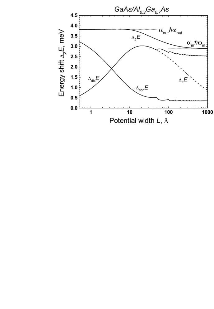
FIG. 1.: Total energy shift $\Delta_{2}E$ is shown vs. the rectangular potential width $L$ for $x=0.3$. The contribution of the discrete ($\Delta_{dis}E$) and continuous ($\Delta_{con}E$) spectra are presented separately as well as the result of the leading term approximation ($\Delta_{lt}E$).

The results of our study for the rectangular potential (which is formed by a layer of $GaAs/Al_{x}Ga_{1-x}As$) are shown in Fig. 1 for the polaronic energy shift and in Fig. 2 for the polaron effective mass at the $AlAs$ mole fraction $x=0.3$. The contribution of the discrete and continuous spectra are plotted separately for this potential. In Fig. 2a the relative mass shift $\Delta_{2}m/m$ is shown where the mean mass $m$ also depends on the potential width $L$. Thus, the ratio $\delta_{2}m=\Delta_{2}m/\Delta_{2}m_{in}$ of the mass shifts in the potential and in $GaAs$ is presented also in Fig. 2b for the same $AlAs$ mole fraction. Evidently, the asymptotics of this curve is equal to the unity at large $L$ and to the ratio $m_{out}\alpha_{out}/m_{in}\alpha_{in}$ at $L\to 0$.

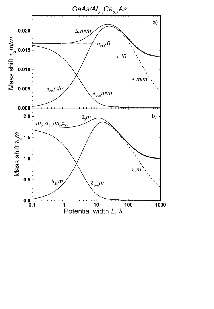
FIG. 2.: The relative shifts $\Delta_{2}m/m$ and $\delta_{2}m=\Delta_{2}m/\Delta_{2}m_{in}$ of the effective polaron mass for the rectangular potential at $x=0.3$. Contributions of the discrete and continuous spectra are shown as well as the result of the leading term approximation.

We may conclude that the continuous spectrum dominates at small potential widths. At large widths its contribution could also be significant although it is smaller than the contribution of the discrete spectrum (especially in deep potential wells). We also confirm the conclusion of the preceding papers that the leading term approximation is not adequate to describe this system and leads to wrong asymptotics at both small and large potential widths (see the dashed lines in Figs 1, 2).

An example of a multilayered heterostructure is presented. The results for the energy and the effective mass for the polaron in the Rosen-Morse potential well are shown in Fig. 3. For the numerical calculations we fix the value $V_{0}=227.9$ meV in Eqs. (79), (83) which corresponds to the limiting mole fraction at large distances $x_{\infty}=\lim_{z\to\infty}x(z)=0.3$. Thus, we obtain the dependence of the mole fraction $x$ on the coordinate $z$:

$$600\cdot(1.155x+0.37x^{2})=227.9\ {\rm tanh}^{2}z.$$ (119)

Now Eqs. (107), (108), (117) allow one to define the dependence of parameters on the coordinate $z$ and to calculate the mean characteristics of the heterostructure.

The calculations were completely different in comparison with the rectangular potential: instead of the direct summation over all intermediate states we used the analytical expression for the Green function of the Rosen-Morse potential. The results obtained demonstrate a similar behavior which is also close numerically to the results for the rectangular potential. The polaronic energy and mass shifts for the rectangular quantum well are also plotted here (dashed line) vs. the Rosen-Morse width $L_{RM}$ obtained from $L$ as is described above. We see that both the energies almost coincide, which gives the opportunity to approximate different quantum wells by the rectangular potential. The discrepancy in the effective mass is larger but not so crucial. This serves also as an additional internal criterion of the validity of our calculations.

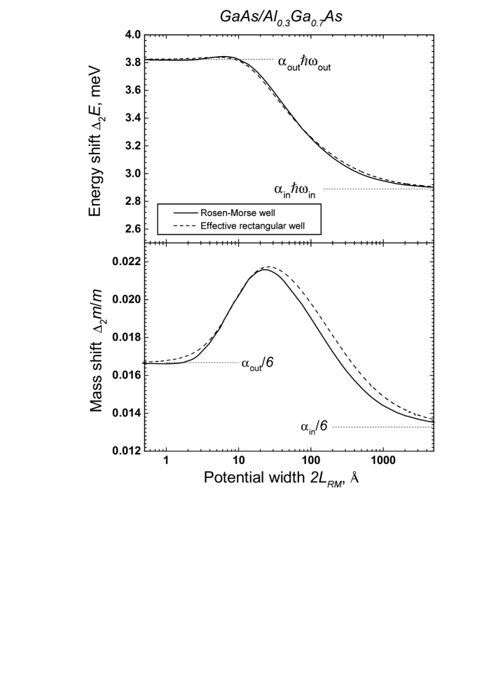
FIG. 3.: Polaron energy and effective mass shifts for the Rosen-Morse potential (solid curves). The dashed lines present results for the rectangular potential at $x=0.3$ as functions of $2L_{RM}$ recalculated from the width $L$ as is described in the text.

Thus, we obtained a monotonous behavior of $\Delta_{2}E$ between the correct 3D limiting values $\alpha_{in}\hbar\omega_{in}$ and $\alpha_{out}\hbar\omega_{out}$ both for the rectangular and the Rosen-Morse potentials (see Fig. 1 and Fig. 3a). Actually the peaks are “hidden” and they reveal themselves if we plot the dimensionless energy shift $\Delta_{2}E/(\hbar\omega_{\mbox{LO}}\alpha)$ which has the same 3D limit (the unity) at both small and large potential widths. But in the “real” units (meV) the peaks are smoothed.

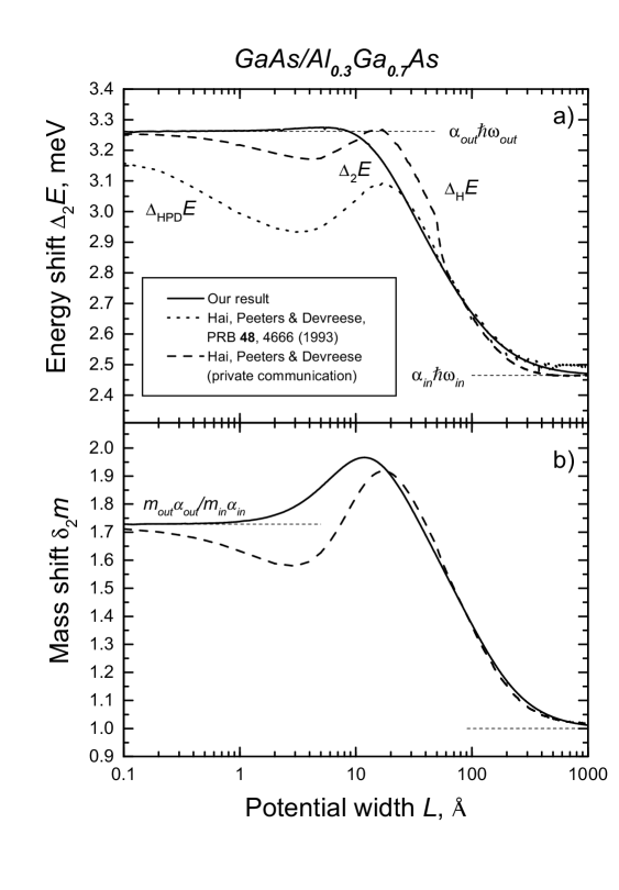
FIG. 4.: Comparison of the results of the present paper (solid lines) and those of Ref. [20] (dotted line) and of Ref. [21] (dashed lines) for the rectangular potential generated by the $GaAs/Al_{0.3}Ga_{0.7}As$ heterostructure. For this plot we used in our calculations the same parametrization (V) and (118) as these authors did.

To compare our results with the calculations performed for the one-layer heterostructure we refer to the papers[20, 21] where the authors took into account the contributions of different phonon modes as well as mass and dielectric constant mismatches in the materials of the barrier and the well. Note that the analytical formulas of Ref. [20] contain a mistake — the wrong expression for the density of states. Namely, in some parts of the continuous spectrum contribution the integration is performed not over the wave vector $p$ but over the wave vector $q$ (that is $\int_{V_{0}}^{\infty}dE_{z}/\sqrt{E_{z}}\,(\ldots)$ in the notations of that paper instead of the correct integration $\int_{V_{0}}^{\infty}dE_{z}/\sqrt{E_{z}-V_{0}}\,(\ldots)$). It is clear that this mistake results in lowering of the resulting curve for the energy, and the discrepancy is larger when the energy is closer to the potential edge, that is at small widths. This is just what we see in Fig. 4a comparing the result of Ref. [20] (the curve $\Delta_{HPD}E$) with the new calculations of the same authors (the curve $\Delta_{HPD}E$) which came to our knowledge when the present paper was already submitted for the publication.

Thus, our model does not reproduce the more complicated structure with the peak and the dip which was obtained in Ref. [21]. Some hints on the existence of peaks can also be seen in our plots but the maximal values are so close to the asymptotics that the peaks are almost invisible. Probably, the dip appears because of the presence of several phonon modes (bulk, interface, etc.). At widths $L\geq 50\ \AA$ our results for the energy practically coincide with those of Ref. [21]. The discrepancy at smaller widths seems to be more crucial. But the difference between the values in the peak and in the dip for the curve $\Delta_{H}E$ in Fig. 4a is about 0.1 eV (3%). This phenomena hardly can be seen experimentally and this discrepancy is in the limits of the accuracy of our model estimated above. This gives indeed a strong support to our model and we may conclude that the latter provides us with the rather accurate approximation and can be used for more complicated calculations in multilayered heterostructures.

As to the shift of the electron band mass we found clear peaks for both the rectangular and the Rosen-Morse potentials (see Figs. 2, 3). As is seen in Fig. 2 the effective mass shift for the polaron in the rectangular quantum well has a peak at $L\approx 20\AA \ (x=0.3)$. Calculations show also that the larger is $x$ the smaller is the potential width corresponding to the peak. For the Rosen-Morse potential at $x_{max}=0.3$ the peaks in the effective mass occur at $2L_{RM}\approx 20\AA$. Note, that again the authors of Ref. [21] obtained curves with peaks and dips in contrast with our results (see Fig. 4b). The maximal discrepancy for the mass is about 11% at $L\approx 3\AA$ which is beyond the region available for experiments. Our results are very close to those of Ref. [21] at $L\geq 10\AA$ and practically coincde with them at $L\geq 20\AA$.

To compare our results with those of Ref. [22] we need now another parametrization used by these authors (although they refer also to the paper by Adachi[25]). Namely, they took a slightly different expression for the confining potential:

$$V(z)=600\cdot(1.266x+0.26x^{2})\ {\rm meV},$$ (120)

which follows from the band gap of Ref. [32]. Furthermore, instead of the effective LO-phonon frequency they used the expression (110) for the energy of the $GaAs$-like phonons. The Fröhlich coupling constant $\alpha$ was calculated then using also the parametrization (107) and (V). Note, that these numerical calculation, as we found, can be approximated by the interpolation formula

$$\alpha(z)=0.0797+0.0772x+0.0295x^{2}.$$ (121)

The results of the comparison are shown in Fig. 5 (we used in our calculations for this plot the same parametrization as was used in Ref. [22]).

The curve $\Delta_{Ch}E$ in Fig. 5a for the energy shift taken from Ref. [22] has also a small dip (qualitatively similar to this of Ref. [21]). But the discrepancy between energy shifts is much more drastic in this case, and we have no explanation for this.

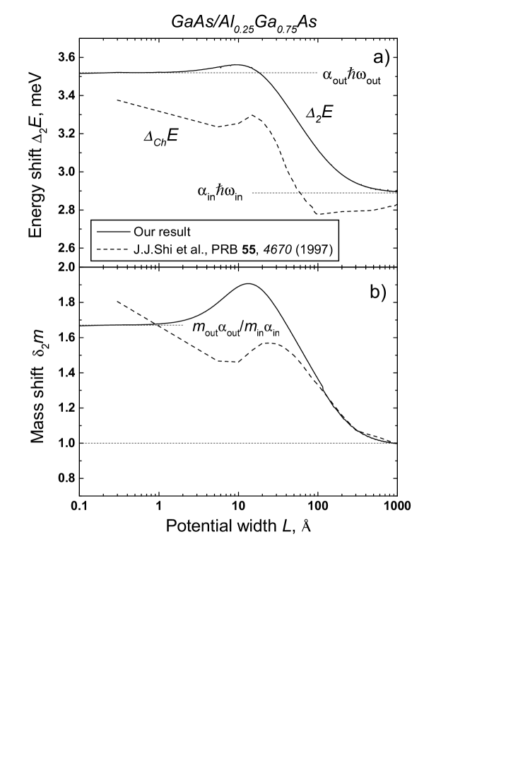
FIG. 5.: Comparison of the results of the present paper and those of Ref. [22] for the rectangular potential generated by the $GaAs/Al_{0.25}Ga_{0.75}As$ heterostructure. For this plot we used the parametrization of these authors as is described in the text.

It is clear that at large potential width only a bulk phonon mode inside the quantum well contributes so these curves should have the same limiting value $\alpha_{in}\omega_{in}$. Numerically we found $\alpha_{in}=0.0797$ and $\omega_{in}=36.25$ meV, so $\alpha_{in}\omega_{in}=2.89$ meV. Moreover, the behavior of the curves at large $L$ should be qualitatively and quantitatively the same which was the case when we compared our model with Refs. [20, 21]. In contrast with our model and the cited results by Hai, Peeters and Devreese the curve $\Delta_{Ch}E$ in Fig. 5b approaches the asymptotics from below and the subsequent mechanism remains unclear. On the other hand there are some reasons why the curve have to approach its asymptotics from above. Indeed, at large potential width the particle does not feel yet the finite height of the potential, and the energy shift takes the same value as in the infinitely high potential which is a bit larger than the free polaron energy.

As to the opposite limit of the small width of the confining potential, it is surprising that the asymptotic value is not reached even at $L\sim 0.3\ \AA ,$ as is found in Ref. [22]. Numerically we obtained $\alpha_{out}=0.1014$ in this scheme and $\omega_{out}=34.72$ meV, so $\alpha_{out}\omega_{out}=3.52$ meV.

Both asymptotic values coincide with what was obtained by the authors of Ref. [22]. Looking at the behavior of the mass shift, we see that both curves coincide at large widths as it should be. At widths smaller than 100 Å the discrepancy becomes evident. But we may conclude that something is wrong with the numerical job of Ref. [22] because their curve approaches the wrong limit at $L\to 0$. Indeed, in this limit the asymptotical value of the plotted ratio should be equal to $\alpha_{out}m_{out}/\alpha_{in}m_{in}$. As it follows from our analysis of the energy shift, we obtained the same values for the Fröhlich coupling constants. The values for the band masses follow from Eq. (107): $m_{in}=0.0665m_{e}$ and $m_{out}=0.0874m_{e}$ at $x=0.25$. Then, the asymptotical value of the plotted ratio should be equal to $1.67$, instead of 1.83 what was found in Ref. [22] That is, the discrepancy is about 10% in this limit and we cannot explain its origin as well.

It would be highly desirable to include a comparison of our results and the results by other authors with corresponding experiments. To the best of our knowledge, no such experiments do exist at the moment.

VI Conclusions

To conclude, we suggested an approximate model to describe a multilayered $GaAs/Al_{x}Ga_{1-x}As$ heterostructure as an effective medium with one (bulk) phonon mode. The fundamental entity is the confining potential generated by these layers which we take into account explicitly. Then we calculate the mean characteristics of the electron in the effective medium (such as its band mass, phonon frequencies etc.) which depend on the form of the confining potential. With these parameters we calculated the energy and the effective mass of a polaron confined to a quasi-2D quantum well $GaAs/Al_{x}Ga_{1-x}As$ for different $AlAs$ mole fractions. The calculations include the full energy spectrum as intermediate states. Peaks are found for the effective mass at some potential widths while the energy demonstrates rather monotonous behavior between the correct 3D-limits. Finally, some discrepancies in the interpolation formulae for the experimental results are discussed as well as discrepancies with the previously obtained theoretical results. We demonstrated that our model gives practically the same (or very close) results as the explicit calculations of Ref. [21] for potential widths $L\geq 10\AA$.

- [1] Electronic mail: smond@thsun1.jinr.dubna.su
- [2] Current address: National High Magnetic Field Laboratory, Florida State University, Tallahassee, Florida, 32304, USA.
- [3] S. Das Sarma and B. A. Mason. Ann. Phys. 163, 78 (1985).
- [4] F. M. Peeters, X. Wu, and J. T. Devreese. Phys. Rev. B 31, 3420 (1985); 33, 3926 (1986)
- [5] O. V. Seljugin and M. A. Smondyrev. Physica A 142, 555 (1987).
- [6] S. Das Sarma. Phys. Rev. B 27, 2590 (1983).
- [7] S. Das Sarma and M. Stopa. Phys. Rev. B 36, 9595 (1987).
- [8] V. V. Bryskin and Yu. A. Firsov. Fiz. Tverd. Tela 13, 496 (1971) [Sov. Phys.—Solid State].
- [9] J. J. Licari and R. Evrard. Phys. Rev. B 15, 2254 (1977).
- [10] V. M. Fomin and E. P. Pokatilov. phys. stat. sol. (b) 132, 69 (1985).
- [11] L. Wendler and R. Pechsted. phys. stat. sol. (b) 138, 196 (1986); 141, 129 (1987).
- [12] L. Wendler and R. Haupt. phys. stat. sol. (b) 143, 487 (1987).
- [13] E. P. Pokatilov, V. M. Fomin, and S. I. Beril. Vibrational excitations, polarons and excitons in multi-layer systems and superlattices (Shtiintsa, Kishinev, 1990).
- [14] V. M. Fomin and E. P. Pokatilov. In: “Formation of Semiconductor Interfaces”. Proc. of the 4th International Conference. Forschungszentrum Jülich, 14-18 June, 1993. — Singapore: World Scientific, 1994, pp. 704 - 707.
- [15] S.N. Klimin, E.P. Pokatilov, and V.M. Fomin, phys. stat. sol. (b), 190, 441 (1995).
- [16] J. J. Licari. Solid State. Commun. 29, 625 (1979).
- [17] X. X. Liang, S. W. Gu, and D. L. Lin. Phys. Rev. B 34, 2807 (1986).
- [18] F. Cosmas, C. Trallero-Giner, and R. Riera. Phys. Rev. B 39, 5907 (1989).
- [19] M. H. Degani and O. Hipólito. Phys. Rev. B 35, 7717 (1989).
- [20] G. Q. Hai, F. M. Peeters, and J. T. Devreese. Phys. Rev. B 48, 4666 (1993).
- [21] G. Q. Hai, F. M. Peeters, and J. T. Devreese. Private communication (May 2000).
- [22] J. J. Shi, X. Q. Zhu, Z. X. Liu, S. H. Pan, and X. Y. Li. Phys. Rev. B 55, 4670 (1997).
- [23] H. Kleinert and I. Mustapić. J. Math. Phys. 33, 643 (1992).
- [24] W. Fischer, H. Leschke, and P. Müller. In: “Path Integrals from meV to MeV: Tutzing ’92”, ed. H. Grabert, A. Inomata, L. S. Schulman, U. Weiss (World Scientific, Singapore, 1993), p. 259; Ann. Phys. 227, 206 (1993).
- [25] S. Adachi. J. Appl. Phys. 58, R1 (1985).
- [26] O. K. Kim and W. G. Spitzer. J. Appl. Phys., 50, 4362 (1979).
- [27] I. Strzalkowski, S. Joshi, and C. R. Crowell, Appl. Phys. Lett., 28, 350 (1976).
- [28] E. Kartheuser. In: “Polarons in Ionic Crystals and Polar Semiconductors”, ed. J. T. Devreese, North-Holland, Amsterdam, 1972; pp. 717-733.
- [29] G.A. Samara, Phys. Rev. B 27, 3494 (1983).
- [30] R. E. Fern and A. Otton, J. Appl. Phys., 42, 3499 (1971).
- [31] H. J. Lee at al. Phys. Rev. B 21, 659 (1980).
- [32] M.A. Afromowitz, Solide State Comm. 15, 59 (1974).