TIGHT-BINDING LINEAR SCALING METHOD APPLICATIONS TO SILICON SURFACES

Abstract

The past years have witnessed impressive advances in electronic structure calculation, especially in the complexity and size of the systems studied, as well as in computation time. Linear scaling methods based on empirical tight-binding Hamiltonians which can describe chemical bonding, and have a computational time proportional to the number of atoms N in the system, are of particular interest for simulations in material science. By contrast conventional diagonalization schemes scale as $N^{3}$. In combination with judiciously fitted parameters and an implementation suited for MD, it is possible to apply such O(N) methods to structural, electronic and dynamical properties of large systems which include up to 1000 atoms on a workstation.

Following a brief review of a tight-binding based linear-scaling method based on a local orbital formulation and of parametrizations appropriate for covalently bonded systems, we present recent test calculations on Si(111)-5 $\times$5 and Si(001)-c(4$\times$2) reconstructed surfaces in this framework, and compare our results with previous tight-binding and ab-initio calculations.

Key words: linear scaling, tight-binding, silicon surface reconstruction.

1 Introduction: Ab Initio vs. Semiempirical, $O(N^{3})$ vs. $O(N)$ Methods

In the past two decades, the percentage of theoretical investigations of materials based on atomistic computer simulations has steadily increased. Those using either an ab-initio or a tight-binding independent electron description of interactions are able to account for chemical bond formation and breaking, and are particularly worthy of attention, as reflected in the 1998 Nobel prize for chemistry. One shortcoming of the usual implementation of such methods is that the number of operations scales as the third power of the number of atoms N, i.e., their computational cost is $O(N^{3})$. Currently this limits the number of atoms in the system that can be treated even using very powerful computers. Ab-initio methods certainly give more precise results than semiempirical tight-binding methods, but besides being based on more complicated Hamiltonians, they require much more extensive basis sets to expand the wave functions of electrons. Empirical tight-binding methods provide a useful compromise between classical empirical potential approaches and ab-initio methods, because they retain a quantum mechanical description of the electrons, ultimately responsible for chemical bonding, but the Hamiltonian is parametrized and the wavefunctions expanded in a minimal set of atomic orbitals. As a consequence, the number of atoms which can be handled with even the simplest ab-initio method, the Local Density Approximation[1] commonly used in materials science is one to two orders of magnitude less than with tight-binding methods within the same computational constraints . Whereas chemists are interested in studying large, complex molecules, materials scientists are concerned with the properties of clusters, solids with specific defects or disorder, surfaces, interfaces, artificial structures and their interactions. Reliable computations of properties require simulations on large enough finite systems, e.g. enclosed in a “box” with periodic boundary conditions applied.

In order to increase the number of atoms in the system and to study dynamical process or finite-temperature properties obtained from time averages, efforts are constantly made to reduce computational cost. For this reason, many kinds of linear scaling methods have been introduced, tested and compared . The interested reader is referred to recent reviews[2, 3]. Linear scaling or O(N) means that the computation time is proportional to the number N of atoms in the system, just like in classical simulations with finite-range interaction potentials[4]. In this contribution we concentrate on a particular orbital-based linear scaling method which, in conjunction with a tight-binding Hamiltonian, has been successfully applied to C and Si systems[5, 6].

This contribution is organized in following way: First we review the approximations and the method, then we present results on $Si(111)-5\times 5$ and $Si(001)-c(4\times 2)$ reconstructed surfaces which serve to validate the method for future applications. At the end we compare our results with previous LDA and tight-binding computations and summarize our conclusions.

2 The Tight-Binding Linear Scaling Method

2.1 Semiempirical Tight-Binding Approximation

The empirical tight-binding (TB) approximation allows the quantum mechanical nature of covalent bonding to enter the interaction Hamiltonian in a natural way rather than through additional ad hoc angular terms in a classical potential.

In TB models the total energy of the system is expressed as

$$E=E_{BS}+\sum_{LL^{\prime}}\phi\left(\left|\mathbf{R}_{L}-\mathbf{R}_{L^{\prime}}\right|\right),$$ (1)

where $\phi$ is a repulsive two-body potential which includes the ion-ion repulsion and the electron-electron interactions which are double counted in the electronic ”band-structure” term $E_{BS}$. This term describes chemical bonding, it can be written as,

$$E_{BS}=\sum_{i}f_{i}\epsilon_{i}=\sum_{i}f_{i}<\psi_{i}\left|\hat{H}_{TB}\right|\psi_{i}>,$$ (2)

where $\hat{H}_{TB}$ is the TB Hamiltonian, $\epsilon_{i}$ and $\{\psi_{i}\}$ are its eigenvalues and eigenstates, and $f_{i}$ is their occupancy. The total number of valence electrons is from now on denoted as N and the total number of single particle states is then N/2 if we assume double occupancy, i.e., spin degeneracy for each state($f_{i}=2$). The occupied eigenstates can in principle be determined by diagonalization, but in our work diagonalization is only used at the very end of each computation to check its accuracy. The off-diagonal elements of $\hat{H}_{TB}$ are described by invariant two-center matrix elements, $V_{ss\sigma},\,V_{sp\sigma},\,V_{pp\sigma}$ and $V_{pp\pi}$, between the set of $sp^{3}$ atomic orbitals(assumed orthonormal). By adjusting their values at the interatomic distance $r_{0}$ = 2.35Å in the equilibrium diamond-like structure, as well as diagonal elements $E_{s}$, $E_{p}$, a good fit to the position and dispersion of the occupied valence bands of Si can be obtained [7].

In order to study properties of covalently bonded systems with defects or free surfaces tight-binding model must be transferable to different physically relevant environments. An important advance was due to Goodwin, Skinner and Pettifor[8] who showed that it is possible to set up a TB model which accurately describes the energy-versus-volume behaviour of Si in crystalline phases with different atomic coordination, and reproduces the structure of small Si clusters.

We therefore adopt the functional form suggested by GSP[8] for the distance dependence of the two-center matrix elements and of the two-body potential:

$$V_{\alpha}(r)=V_{\alpha}(r_{0})\left(\frac{r_{0}}{r}\right)^{n}exp\left\{n\left[-\left(\frac{r}{r_{c}}\right)^{n_{c}}+\left(\frac{r_{0}}{r_{c}}\right)^{n_{c}}\right]\right\}$$ (3)

$$(\alpha\,:\,ss\sigma,\,sp\sigma,\,pp\sigma,\,pp\pi)$$

$$\phi(r)=\phi_{0}\left(\frac{r_{{}_{0}}}{r}\right)^{m}exp\left\{m\left[-\left(\frac{r}{d_{{}_{c}}}\right)^{m_{{}_{c}}}+\left(\frac{r_{{}_{0}}}{d_{{}_{c}}}\right)^{m_{{}_{c}}}\right]\right\}$$ (4)

where $r$ denotes the interatomic separations, and $n<<n_{c}$, $m<<m_{c}$, $r_{c}\approx d_{c}>r_{0}$ and $\phi_{0}$ are parameters which are determined by fitting judiciously chosen properties. The resulting high values of $n_{c}$, $m_{c}$ ensure a rapid decay of $V_{\alpha}(r)$, $\phi(r)$ beyond $r_{c}$, $d_{c}$. In molecular dynamics(MD) simulations where a finite range of $r$ is explored, the quantities in Eqs.(3-4) are further multiplied by a smoothed step function which switches from 1 to 0 in a narrow interval about a cutoff radius $r_{m}>r_{c},d_{c}$.

As explained below, similar couplings between Si and H atoms are required in some of our computations. Because hydrogen has a single occupied s-state, only $ss\sigma$ and $sp\sigma$ matrix elements must be parametrized. $H-H$ couplings are negligible at the separations considered here.

2.2 Tight-Binding Parameters

Within the above framework, improved sets of parameters were subsequently developed for Si-Si and Si-H interactions. In this contribution, we used the two different sets of parameters described in detail by Kwon et al[9] and Bowler et al[10].

The Si-Si parametrization of Kwon et al[9] is rather complicated; thus $r_{c}$’s, $n_{c}$’s depend on $\alpha$ and the repulsive contribution is represented by a nonlinear function of the second term in Eq.(1). The parameters are fitted to many properties of Si in the diamond structure and to computed(LDA) cohesive energies vs. density of four different structures. The resulting properties of liquid Si and of small Si clusters are in remarkable agreement with experiments and with ab-initio computations. On the other hand, this parametrization uses a cut-off which is beyond second nearest neighbours; this implies significantly larger computing times. The revised GSP parametrization of Bowler et al [10] is less complicated than the previous one; Si-Si parameters were fitted to fewer properties in the diamond and $\beta$-tin structures, Si-H parameters to properties of $SiH_{4}$. Furthermore, the cut-off radius $r_{c}$ can be chosen between nearest and next-nearest-neighbours; thus this parametrization is very well suited for linear scaling computations. It has in fact been successfully applied to defects and hydrogen diffusion on Si(001) [10].

2.3 Orbital Based Linear Scaling Energy Minimization without Orthogonalization Constraints

Traditional electronic structure methods solve the Schrödinger equation by expanding one-electron wavefunctions in a fixed basis set (plane waves, atomic orbitals or combinations thereof) and by diagonalizing the resulting secular equation for the expansion coefficients. In spite of significant progress achieved by applying efficient diagonalization algorithms, the required computing time is proportional to $NP^{2}$, P being the number of basis functions. Because $P\propto N$, the computational cost is $O(N^{3})$, the scaling factor depending on the method, being small in the case of empirical tight-binding. Nevertheless, the diagonalization of $\hat{H}$ for each atomic geometry or at each step of MD simulation limits the number of atoms that can be currently studied in conventional TBMD computations to about 100 using a workstation and around 1000 using a supercomputer. The recently developed linear scaling methods compute the total energy by minimizing a functional expressed in terms of localized orbitals in real space. Although typical eigenstates in a condensed system extend throughout most of it, a unitary transformation yields linear combination of the former which are localized about particular sites. On the basis of exact model calculations [11], these so-called Wannier orbitals are believed to decay exponentially in systems with a finite energy gap between occupied and empty states [12]. This applies in particular to the finite systems on which computations are carried out, although the effective gap can be small and corresponding decay slow if the corresponding real system is metallic.

The key feature of $O(N)$ methods is that the total energy and the forces acting on individual atoms are evaluated without computing the eigenvalues and eigenstates of $\hat{H}$. This is accomplished by dividing the full system into finite subsystems and by defining localized orbitals  {$\phi$} which are forced to vanish outside each subsystem[13]. These localized regions (LR) are the electronic equivalents of the linked cells which ensure O(N) scaling in classical simulation[4]. Intuition and experience suggest that the minimum size of each localization region depends on physical and chemical properties of the constituents, and not on the size of the system whole. The size of the localized regions (which must exceed the range of $\hat{H}$) is always the factor which limits the accuracy of an $O(N)$ calculation.

Another key ingredient to achieve $O(N)$ scaling is the definition of an appropriate energy functional whose minimization requires neither explicit orthogonalization of the auxiliary electronic orbitals, nor the inversion of their overlap matrix $\mathbf{S}$. This functional is in general different from that defined in Eq.(1), but must have the same global minimum in the limit of infinite localization regions. Otherwise it yields an upperbound which in practice, must be close to the minimum energy even for relatively small LR’s. This can in fact be achieved [2, 3, 6]. Various O(N) methods are based on different functionals which, however, share this remarkable property.

One convenient energy functional which satisfies these requirements is [6]:

$$E_{GBS}\left[\left\{\phi\right\},\mu,M\right]=2\sum^{M}_{ij=1}(2\delta_{ij}-S_{ij})<\phi_{j}\left|\hat{H}-\mu\right|\phi_{i}>+\mu N$$ (5)

The matrix $(2I-S)$ is the first order truncated series expansion of the inverse overlap matrix $S^{-1}$, where $S_{ij}=<\phi_{i}|\phi_{j}>$. The functional defined in Eq.(5) depends on the number M localized orbitals (LO), and on a global variable $\mu$ which determines the highest filled state and hence the total electronic charge in the system at the minimum. Taking $M>N/2$ helps avoid unphysical solutions [6], depending on the initial choice of the orbitals, which can otherwise be obtained.

In order to find the electronic ground state energy for a given spatial configuration of the atoms, the functional is minimized with respect to the LO’s. Normally each LR is centered at an atomic site I and encompasses all neighbours connected by n bonds; it is then denoted by nLR. Then LO $\phi_{i}$ centered at atomic site I can be expressed as

$$\phi_{i}=\sum^{n_{b}}_{J\in\{LR_{I}\}}\sum_{l}C_{Jl}^{i}\alpha_{Jl}$$ (6)

where $\alpha_{Jl}$’s are the atomic basis functions of atom J, the index l runs over orbital components (e.g. $s,\,p_{x},\,p_{y},\,p_{z}$ for carbon or silicon and s for H), $\{LR_{I}\}$ indicates the set of atoms within the localization region centered at site I, and $n_{b}$ is the corresponding number of basis functions.

The functional is efficiently minimized using a conjugate gradient (CG) algorithm[14]. The required derivatives

$$\frac{\partial E_{GBS}}{\partial\phi_{i}}=4\sum_{j}^{M}\left[\left|(H-\mu)\phi_{i}>(2\delta_{ij}-S_{ij})-\left|\phi_{j}><\phi_{j}\left|(H-\mu)\right|\phi_{i}>\right.\right.\right]$$ (7)

are evaluated at each iteration step. Using Eq.(6) the matrix elements can be expressed in terms of the Slater-Koster energy integrals $<\alpha_{Jl}|\hat{H}_{TB}|\alpha_{J^{{}^{\prime}}l^{{}^{\prime}}}>$ [15]; those energy integrals can be further expressed in terms of direction cosines and of the invariant two-center matrix elements defined by Eq.(3)(see Appendix B). Because each derivative needs to be evaluated only in the localization region $\{LR\}_{I}$, the required number of operations scales linearly with the number of atoms in the system. The global variable $\mu$ is initially chosen well above the estimated Fermi energy of the system, then iteratively adjusted until the total charge of the system becomes equal to the charge consistent with global neutrality when convergence is achieved, i.e., the ground state energy corresponding to the assumed LRs is attained, and $\mu$ is the chemical potential (Fermi energy) of the electrons[6].

2.4 Total Energy Minimization with Respect to Atomic Positions and Electronic Readjustment

In this work we consider only known metastable structures of silicon surfaces in order to test the performance and accuracy of the method. To determine such structures, atoms in several surface layers are allowed to move under the influence of the forces

$$F_{I}=-\partial E/\partial R_{I}$$ (8)

until all their components become smaller than a preset tolerance (0.01 eV/Å) and the energy E reaches a minimum. Instead of using a standard minimization procedure, this is achieved by introducing a damping term in the standard Verlet algorithm [4]. This term is adjusted so that the resulting motion is almost critically damped, so that the fastest possible relaxation is achieved.

Eq.(8) is physically meaningful only if the electrons are in their ground state (Born-Oppenheimer approximation). Therefore, molecular dynamics can be started only after electronic convergence with respect to the initial atomic configuration has been achieved as described in section 2.3. This rather tedious procedure is necessary at the start of a calculation. The required computing time depends on the initial choice of the LOs and $\mu$. To be safe, we start with random coefficients in Eq.(6) and a high $\mu$. To ensure stable MD integration, the time step must be small compared to a typical optical vibration period. The corresponding atomic displacements are then small and typically do not strongly perturb the LO coefficients, except if same atom(s) move out or into certain LRs. Therefore, after each atom move enough electronic iterations must be performed in order to reach the slightly modified ground state (within a relative tolerance $<10^{-4}$). Fortunately, only small adjustments of $\mu$ are necessary once global charge neutrality has been established; they can be performed automatically. The number of electronic steps depends on the system, the narrower its energy gap at the Fermi level(always existing in a finite system), the more electronic steps are needed. Useful O(N) performance is achieved if this number of electronic iterations is independent of N and if the necessary computing time is less than that required for diagonalization.

2.5 Local charge neutrality

If significant atomic rearrangements occur in the course of a molecular dynamics simulation, it is sometimes difficult to avoid unphysical charge transfer between neighboring atoms or layers. To reduce such effects, which slow down convergence and sometimes lead to unphysical solutions, local charge neutrality can be approximately imposed by adding an extra term $H_{U}=\frac{1}{2}U\sum_{I}(q_{I}-q_{I}^{0})^{2}$, where $q_{I}^{0}=4.0$ for Si and 1.0 for H atoms, and the charge around site I is expressed as

$$q_{I}=2\sum_{ij}(2\delta_{ij}-S_{ij})<\phi_{i}\left|\mathbf{R}_{I}><\mathbf{R}_{I}\right|\phi_{j}>$$ (9)

where $<\phi_{i}|\mathbf{R}_{I}>$ indicates the projection of the localized orbital $\phi_{i}$ on the localized region around site I [6]. Such a term is obtained by making a local mean field approximation to the Hubbard Hamiltonian and assuming no spin-polarized solutions[16]. The strength U of the Hubbard-like term has been estimated and tabulated by Harrison[17] who also discussed its reduction by dielectric polarization. In covalent systems such Hubbard-like contributions must essentially vanish once convergence is achieved, for atoms which have a bulk-like environment.

3 Applications

In this section we present our recent test calculations with the method described above which has hitherto been mainly applied to carbon systems. Our ultimate goal is to simulate atomic force microscopy(AFM) and manipulation with a Si tip. We present and discuss our results on Si(111) and Si(001) surface reconstructions which have previously been studied by tight-binding and ab-initio methods, and exhibit characteristic features due to rebonding of surface atoms. Such reconstructions reduce the density of energetically unfavourable ”dangling bonds” on surface atoms, but induce distortions from the tetrahedral bonding pattern in the bulk. Optimum surface structures represent a delicate balance between different effects and can not usually be guessed by chemical and physical intuition.

These reconstructed surfaces are therefore well-suited for validating the method and are also interesting candidates for controlled atom manipulation experiments. Surface properties are extracted from computations on slabs with a finite number of layers. This number must be large enough to suppress artificial coupling between the free slab surfaces which can arise owing to the overlap of surface states and/or to strain fields induced by atomic rearrangements in surface layers. In order to approximate the effect of the crystalline substrate, atoms in the two centeral layers are held in their bulk positions. Alternatively, the bottom two layers are fixed, and all exposed dangling bonds are passivated with hydrogen atoms so as to preserve tetrahedral coordination. Similar accuracy is expected with half the number of free layers, compared to the former, symmetric slab. Having this in mind, we have investigated the influence of factors which, if chosen properly, should have little effect on physical meaningful results. This includes the number of free and fixed (bulk-like) layers in the slabs used, the influence of H-passivation at the bottom, the shape and lateral dimensions of the computational supercell, the size of the localization regions, the tight-binding parametrization, starting from configurations which had the periodicity and some of the rebonding characteristics of desired reconstructions. All this required many computations which were performed on not too large systems in order to economize computing time. Thus the emphasis here is on validation rather than on achieving O(N) performance, although this was demonstrated in the larger systems containing a few hundred atoms.

3.1 Si(111)-5x5 Reconstruction

The metastable 5$\times$5 reconstruction plays an important role in the conversion from 2$\times$1 reconstruction, obtained upon cleavage, to the stable 7$\times$7 reconstruction of the Si(111) surface [18]. It exhibits the characteristic features of the DAS model first proposed for Si(111)-7x7 [19], which are indicated in Fig. 1.

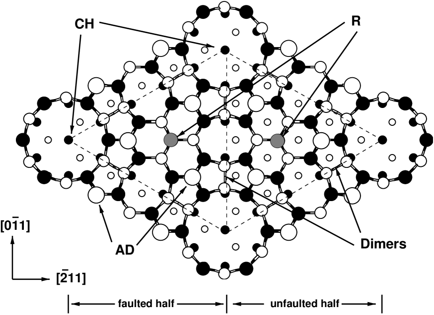
Figure 1: Top view of Dimer-Adatom-Staking fault structure of the Si(111)-5 $\times$5 reconstruction. Circles of decreasing diameter denote atoms in successive layers starting from the top. Large white ones are adatoms, large black and grey ones belong to the first layer with a stacking fault on the left half, smaller white ones belong to the dimer layer, small black ones appear at the center of corner holes and adjacent to the dimers, whereas remaining third layer atoms are hidden under the adatoms, and small white ones belong to the fourth layer. Adatoms(AD), rest atoms(R), corner holes(CH) atoms and the boundary of the surface unit cell are indicated. The thin dotted-dashed line along the short diagonal divides the faulted and unfaulted halves.

One important difference is that the 5$\times$5 reconstruction has the same average density of atoms in surface layers as the bulk terminated Si(111) surface, whereas additional Si adatoms must be supplied to form the 7$\times$7 reconstruction.

3.1.1 Computational Details

We start with a ten-layers thick inversion-symmetric slab which has two bulk truncated (111) surfaces at the top and bottom, encompassing two adjacent 5$\times$5 surface unit cells. Periodic boundary conditions are then maintained in the lateral directions. We have also repeated some of the computations with a six-layers slab passivated by H atoms at the bottom, similar to that used by Adams and Sankey [20]. Following these authors, the initial configuration on the free surface(s) is set up by laterally shifting ten atoms in the surface layer on the left side of each 5$\times$5 cell so that they are placed above fourth layer atoms. Then five atoms at one edge of the other ”unfaulted” triangular half and the second-layer atom above the ”corner hole” are placed at the positions of the adatoms so that their bond lengths to the nearest first-layer atoms are equal to the bulk interatomic distance $r_{0}$. During the combined relaxation of electrons and ions, dimers spontaneously formed along the boundaries between “faulted” and “unfaulted” halves shortly after we started the damped molecular dynamics calculation. At the end, we obtained the relaxed structure consistent with the DAS model illustrated in Fig.1. Of the 25 dangling bonds per 5$\times$5 cell on the truncated (111) surface only 9 are left: one on the corner hole atom (CH), two on the restatom(R) and six on the adatoms(AD). The former three are doubly occupied, whereas surface states derived from those on the adatoms are partially occupied by the remaining three electrons [20]. Thus one expects the $Si(111)-5\times 5$ surface have metallic properties just like $Si(111)-7\times 7$. As a matter of fact, a posteriori diagonalization revealed a tiny ”energy gap” ($<0.01eV$) in our relaxed structure. One might also expect problems due to the assumed double occupancy. In fact relaxation in a slab encompassing a single $5\times 5$ surface unit cell produced a distorted DAS structure with twisted dimers. On the other hand, no such distortions have been found in previous $O(N^{3})$ computations of $Si(111)-7\times 7$ with similar slabs which relied on occupied eigenstates at the $\Gamma$-point(zero wave-vector) obtained by diagonalization [21] or [22, 23, 24] by total energy minimization with orthonormality constraints [25, 26]. Deviations might arise owing to the small size of the localization region(n=3) in our O(N) computations. Fortunately this is not the case, as discussed in the following section, if slabs encompassing on even number number of dangling bonds on each surface are used.

3.1.2 Relaxed Geometry

Our relaxed configuration exhibits common characteristic features found in previous computations of the $5\times 5$ [20, 22] and of the $7\times 7$ [21, 23, 24] reconstructions. In what follows we compare results obtained with Bowler’s parametrization, localization regions encompassing third neighbours and a $5\times 10$ computational cell containing four free layers (not counting the adatoms) and two fixed Si layers with the bottom one saturated by H atoms. In order to check the influence of free and fixed(bulk-like) layers in the slab, of passivation by H at the bottom, of the size of the localization regions, and of the tight-binding parametrization we have performed many calculations of the relaxed geometry of the $5\times 5$ reconstruction. From the result summarized in Appendix A one can conclude that the influence of these factors on the final configuration is negligibly small. This is a very encouraging result. Furthermore the bond lengths listed in Table 1 are remarkably close (except for dimers) to those found in recent TB calculations for the $7\times 7$ reconstruction based on a symmetric slab with one free layer less on each side [24]. Small deviations occur, however, compared to bond lengths extracted from a LDA computation for the same system [23]. Similar deviations also occur compared to an earlier TB computation for a H-passivated slab with two less free layers [21]. In that case, these deviations might be due to that restriction or to the somewhat different parametrization. More significant deviations appear when height differences between adatoms and rest atoms in the two halves of the surface unit cells are compared(see Table 2). Our computed differences are larger than those found in previous computations for the $7\times 7$ reconstruction with a smaller number of free layers. On the other hand, height difference between adatoms is only half of that found in a pioneering computation for $Si(111)-5\times 5$ based on a H-passivated slab like ours [20]. However, in contrast to that work, we found that adatoms in each half are equivalent, just like corner hole and central adatoms are on the $Si(111)-7\times 7$ surface. These two discrepancies are probably due to the non self-consistent LDA-based approximation used in Ref. [20]. TB computations, including ours, are only rudimentary self-consistent if the Hubbard term is included, but since the parameters are fitted to experimental data [10] and/or self-consistent LDA computations [9], they can yield better results.

Table 1: Computed average bond lengths(in Å) between Si atoms in surface layers of $Si(111)-5\times 5$(present) and $7\times 7$ reconstructions. Here 1 - Adatom-first layer atom; 2 - Adatom-second layer atom; 3 - Rest atom-second layer atom; 4 - Dimer; 5 - Dimer-third layer atom; 6 - Corner hole-fourth layer atom

Bonds	present	Kim et al[24]	Qian et al[21]	Brommer et al[23]
1	2.550	2.58	2.486	2.49
2	2.575	2.57	2.471	2.474
3	2.435	2.43	2.410	2.376
4	2.417	2.45	2.463	2.456
5	2.39	2.39	2.405	2.396
6	2.408			2.40

Table 2: Computed height differences(in Å) between adatoms(AD) and rest atoms(R) in the faulted and unfaulted halves of the $5\times 5$ and $7\times 7$ Si(111) surface unit cells. For the $7\times 7$ reconstruction, the two values given refer to the adatoms near corner holes and near the centers of each half cell.

Atoms	Present	Adams et al	Qian et al	Brommer et al
adatoms	0.08	0.17	0.055, 0.07	0.047,0.030
rest atoms	-0.05	-	-0.01	0.03

3.1.3 Convergence, Accuracy and Determination of Surface Energies

The accuracy, efficiency and performance of our O(N) TB computations can be judged on the basis of the results reported in Table 3 for the system described in the preceding section.

Table 3: Comparison of total energies required computation times and numbers of iterations for a system of 300 Si and 50 H atoms

Relaxation	Quantity	2 LR	3 LR	Diagonalization
Initial	Total Energy(eV)	-12896.83	-12918.38	-12932.55
(Electrons)	Computation time(hrs.)	4.5	23
	CG steps	3400	5500
Electrons	Total Energy(eV)	-12958.05	-12977.68	-12987.32
and Atoms	Computation time(hrs.)	6.5	22
	MD steps	1848	1778

Computations were performed on a single processor of a DEC-Alpha 8400 machine; nLR refers to unconstrained minimizations with localization regions encompassing neighbours connected by n bonds. Diagonalization was performed at the end of the 3LR minimization. The first three rows refer to the unbiased but costly minimizations starting with orthonormalized LOs with random coefficients for the initial configuration. It is gratifying that the subsequent combined optimization of LO coefficients and atomic positions takes about the same time. More importantly the ratio of CG to MD steps implies that only three CG steps per MD step are on the average required to reconverge the coefficients.

A comparison of the last two columns suggests that 3LR minimization yields total energies with a relative accuracy of about $10^{-4}$. The specified tolerance on the relative energy difference between successive CG iterations(our convergence criterion) was, of course, much smaller. Note that diagonalization yields eigenstates corresponding to the $\Gamma$-point of the computational supercell. More accurate total energies could be obtained by including occupied eigenstates with nonzero parallel wave-vectors in Eq.(2) or by increasing the lateral dimensions of the supercell(the only alternative in the case of O(N) computations). The surface energy differences $\Delta E_{s}$ which determine the relative stability of possible reconstructions are usually approximated by differences between total energies per projected $1\times 1$ surface unit cell computed in the same computational slab with the desired reconstruction on one face and same reference structure on the other. This approximation is reasonable if the system is sufficiently large, in particular to effectively decouple the two faces. On the other hand, an upper bound on the error in $\Delta E_{s}$ is given by the product of the number of layers times the energy per unit cell of the substrate times the relative accuracy. According to Table 3 this amounts to $\approx 0.05eV$. Computed values of $\Delta E_{s}$ at the 3LR level with respect to the truncated Si(111) surface are only -0.19 eV and -0.13 eV for the symmetric and H-passivated slabs described in section 3.1.1. The difference between those two values is disturbingly close to our estimated error bound. Furthermore, previous estimates of surface energy differences between the $5\times 5$ and the $2\times 1$ and $7\times 7$ reconstructions, which are relevant for understanding their growth [18], from self-consistent LDA computations amount to -0.06 eV [23] and 0.02 eV [22], respectively. This implies that O(N) computations beyond the 3LR level of accuracy will be required to distinguish them reliably. On the positive side, note that $\Delta E_{s}$ = -0.15 eV is found upon diagonalization for both above-mentioned slabs. Finally, the rather different values of $\Delta E_{s}$ obtained in Refs. [21] and [20], namely -0.395 eV and 0.56 eV, suggest that TB parameterization and non-selfconsistency are delicate issues which should be addressed.

3.2 Si(001)-c(4x2) Reconstruction

A truncated 1$\times$1 Si(001) surface contains many unsaturated bonds and the system tends to minimize its energy by reconstructing its surface. Theoretical[27, 28, 29] and experimental[30] evidence shows that this reconstruction causes dimers to appear on the surface; i.e. surface atoms move toward each other to form pairs. Furthermore, these dimers are tilted and asymmetric with respect to terminated bulk. The dimers can arrange themselves in various patterns on the surface and thus many reconstructions of the surface are possible.

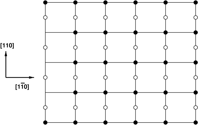
(a) ideal surface

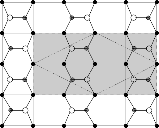
(b) reconstructed surface

Figure 2: Top views of the unreconstructed (bulk truncated) Si(001) surface and of its c(4$\times$2) reconstruction. The shadowed area delimits the surface unit cell used in our simulation. Black circles denote second layer atoms, grey and white circles denote dimerized surface atoms. The white atoms lie higher than the grey counterparts. The primitive c(4$\times$2) surface unit cell is outlined by the dot-dash line in (b).

We have made a less extensive set of O(N) computations for the Si(001) surface. Following a period of controversy, several LDA studies, in particular the exhaustive one of Ramstad et al [31] have confirmed that the $Si(001)-c(4\times 2)$ reconstructions schematically illustrated in Fig.2(b), and first predicted in a pioneering TB computation [27], has in fact the lowest energy. The $p(2\times 2)$ structure, characteristic by identical [110] rows with alternatively tilted Si-dimers, is only marginally metastable, while the 2$\times$1 structure with untilted, symmetric dimers is unstable at low temperatures and 0.1 eV higher in energy per projected (1$\times$1) surface unit cell [31].

We report O(N) computations performed with Bowler et al [10]’s parameterization, n=3 LRs in the 4$\times 2$ surface unit cell indicated by shading in Fig.2(b). Our computational slab consisted of 6 free Si layers and two fixed layers, with the pairs of dangling bonds at the bottom passivated by H atoms in order to approximate a connection to the bulk crystalline silicon substrate. Starting from a configurations with slightly preformed untilted dimers, our computations converged towards a $c(4\times 2)$ reconstruction, although the $p(2\times 2)$ was obtained in some cases.

Table 4: Computed atom displacements from ideal truncated bulk positions (in Å)

	Tight-binding calculations						LDA calculations
Layer	present			Chadi[27]			Ramstad et al[31]			Northrup[32]
	$\Delta x$	$\Delta y$	$\Delta z$	$\Delta x$	$\Delta y$	$\Delta z$	$\Delta x$	$\Delta y$	$\Delta z$	$\Delta x$	$\Delta y$	$\Delta z$
1	0	0.629	0.045	0.	0.46	0.04	0	0.68	-0.05	0	0.61	-0.04
1	0	-0.821	-0.383	0.	-1.08	-0.435	0	-0.95	-0.788	0	-1.04	-0.74
2	0.09	0.115	-0.011	0.	0.115	-0.014	0.117	0.12	-0.086	0.008	0.1	-0.07
2	-0.09	-0.115	-0.01	0.	-0.115	-0.014	-0.12	-0.108	-0.079	-0.008	-0.1	-0.07
3	0.	0.	-0.2	0.	0	-0.12	0	0.009	-0.223	0	0	-0.19
3	0.008	0.	0.117	0.	0	0.11	0.02	0.003	0.066	0.001	0	0.05
4	0	0.023	-0.132	0.	0	-0.07	0	0.006	-0.154	0	0	-0.12
4	0	0.	0.08	0.	0	0.07	0	0.005	0.069	0	0	0.04
5	0	0.049	-0.01	0.	0.034	0.	0	0.043	-0.03
5	0	-0.067	-0.31	0.	-0.034	0.	0	-0.038	-0.03

As can be seen from Table 4, the resulting pattern of atomic displacements is reproduced correctly, the relaxed coordinates being within the spread of values from previous computations. Relevant deviations are more evident in Table 5. The dimer tilt, being energetically easy, is quite sensitive to the level of approximations. The deviation of the dimer bond length from the bulk Si-Si distance(2.35Å), in the opposite direction to LDA prediction is more serious and disappointing. Indeed, Bowler et al [10] claimed that their parameterization would cure this discrepancy. More computations are needed to check the extent to which the above-mentioned deviations are affected by computational approximations, and to extract reliable surface energy differences.

Table 5: Computed bond lengths and tilt angle of surface dimer.

Bonds	present	Ramstad et al[31]	Chadi[27]
I	2.425	2.29	2.35
II	2.345	2.31	2.332
III	2.367	2.35	2.390
IV	2.379	2.37	2.398
V	2.377	2.35	2.34
$\alpha$	10.2o	18.8o	11.68o

Inset: Side view of tilted dimer and of second and third layer atoms

A posteriori diagonalization gives a 0.9 eV band gap, a value which is reasonable [32], but should not be taken too seriously because the TB parameters are fitted to occupied valence bands and to ground-state properties. The existence of a band gap is consistent with the known semiconducting nature of the $c(4\times 2)$.

4 Conclusions

Summarizing the results described in section 3 and Appendix A, we conclude that the local-orbital-based linear scaling TB scheme proposed by Kim et al [6] reproduces the correct configurations of representative silicon surface reconstructions. Except for a few discrepancies which can be traced to inadequencies of the tight-binding description itself, satisfactory geometries are obtained with the simpler parametrization of Bowler et al [10] and with local orbitals constrained to vanish beyond second nearest neighbours. This even applies to the metallic $Si(111)-5\times 5$ surface provided that the computational surface unit cell encompasses on even number of dangling bonds. These encouraging results open the door to applications to larger systems exploiting the linear-scaling capability of this new computational scheme, e.g. involving interactions on and between silicon clusters and surfaces exposing different faces with or without passivating hydrogen atoms.

It is, however, important to keep in mind that a higher level of accuracy appears required to quantitatively describe surface energy differences between alternative (meta)stable structures. This aspect is currently under study.

5 Acknowledgements

This work was supported by the Swiss National Foundation for Scientific Research under the programm NFP36 ”Nanosciences”. The first two authors are grateful for the facilities and services provided by the computing center and the Institute of Physics of University of Basel. They wish to thank Prof. H.-J. Güntherodt for his encouragement, D. Bowler and R. Härle for discussions.

Appendix A Influence of Various Factors

As explained in section 2.3, the use of local orbitals assumed to vanish outside finite localization regions is main approximation leading to linear scaling. O(N) TB computations are efficient if the range of TB interactions and size of the LR(the number of neighbours connected to the central atom by n bonds) can be chosen as small as possible without unduly sacrificing accuracy. For this reason we have performed test calculations with n=2 and n=3 LRs for the two TB parametrizations described in section 3.1 and different slabs. Representative bond lengths obtained for the $Si(111)-5\times 5$ reconstruction are shown in Table 6. Column 1 and 2 show the results obtained with the complex and simpler parametrizations using a symmetric slab with 8 layers(not counting adatoms) and n=3 LRs. Column 3 shows the results obtained with the same LR and using TB parameters as in column 2 but for a slab with 6 layers, passivated by hydrogen atoms at the bottom. Column 4 shows results obtained with for the same TB parameters and slab as in column 3, but using n=2 LRs. From the results one can see that these factors have little influence on the final relaxed geometry.

Table 6: Comparison of bond lengths in surface layers of the $Si(111)-5\times 5$ reconstruction computed for different TB parametrizations, slab and localization regions. Here 1 - Adatom-first layer atom; 2 - Adatom-second layer atom; 3 - Rest atom-second layer atom; 4 - Dimer; 5 - Dimer-third layer atom; 6 - Corner hole-fourth layer atom

	parametrization (symmetric slab, 3 LR)		LR(with H, Bowler et al’s)
Bonds	Kwon et al [9]’s	Bowler et al [10]’s	3 LR	2 LR
1	2.545	2.56	2.550	2.545
2	2.58	2.58	2.575	2.580
3	2.44	2.44	2.435	2.446
4	2.41	2.42	2.417	2.414
5	2.39	2.39	2.39	2.39
6	2.44	2.41	2.408	2.410

Appendix B The matrix element $<\alpha_{Jl}|\hat{H}_{TB}|\alpha_{J^{{}^{\prime}}l^{{}^{\prime}}}>$

When $J=J^{{}^{\prime}}$, the matrix is given by

$$<\alpha_{Jl}|\hat{H}_{TB}|\alpha_{J^{{}^{\prime}}l^{{}^{\prime}}}>=\left\{\begin{array}[]{ll}E_{s}&\begin{array}[]{ll}if&l=l^{{}^{\prime}}=s\end{array}\\ E_{p}&\begin{array}[]{ll}if&l=l^{{}^{\prime}}=p_{x},p_{y},p_{z}\end{array}\\ 0&\begin{array}[]{ll}if&l\neq l^{{}^{\prime}}\end{array}\end{array}\right.$$

When $J\neq J^{{}^{\prime}}$, the various matrix elements can be written as,

$$E_{Js,J^{{}^{\prime}}s} = V_{ss\sigma}$$ (10)

$$E_{Js,J^{{}^{\prime}}p_{x}} = -E_{Jp_{x},J^{{}^{\prime}}s}\;=\;lV_{sp\sigma}$$

$$E_{Js,J^{{}^{\prime}}p_{y}} = -E_{Jp_{y},J^{{}^{\prime}}s}\;=\;mV_{sp\sigma}$$

$$E_{Js,J^{{}^{\prime}}p_{z}} = -E_{Jp_{z},J^{{}^{\prime}}s}\;=\;nV_{sp\sigma}$$

$$E_{Jp_{x},J^{{}^{\prime}}p_{y}} = -E_{Jp_{y},J^{{}^{\prime}}p_{x}}\;=\;lm(V_{pp\sigma}-V_{pp\pi})$$

$$E_{Jp_{x},J^{{}^{\prime}}p_{z}} = -E_{Jp_{z},J^{{}^{\prime}}p_{x}}\;=\;ln(V_{pp\sigma}-V_{pp\pi})$$

$$E_{Jp_{y},J^{{}^{\prime}}p_{z}} = -E_{Jp_{z},J^{{}^{\prime}}p_{y}}\;=\;mn(V_{pp\sigma}-V_{pp\pi})$$

$$E_{Jp_{x},J^{{}^{\prime}}p_{x}} = E_{Jp_{x},J^{{}^{\prime}}p_{x}}\;=\;l^{2}V_{pp\sigma}+(1-l^{2})V_{pp\pi}$$

$$E_{Jp_{y},J^{{}^{\prime}}p_{y}} = E_{Jp_{y},J^{{}^{\prime}}p_{y}}\;=\;m^{2}V_{pp\sigma}+(1-m^{2})V_{pp\pi}$$

$$E_{Jp_{z},J^{{}^{\prime}}p_{z}} = E_{Jp_{z},J^{{}^{\prime}}p_{z}}\;=\;n^{2}V_{pp\sigma}+(1-n^{2})V_{pp\pi}$$

here $l,m,n$ are the direction cosines of the vector $\mathbf{R}_{J^{{}^{\prime}}}-\mathbf{R}_{J}$:

$$l=\frac{R_{J^{{}^{\prime}}x}-R_{Jx}}{|\mathbf{R}_{J^{{}^{\prime}}}-\mathbf{R}_{J}|}$$

$$m=\frac{R_{J^{{}^{\prime}}y}-R_{Jy}}{|\mathbf{R}_{J^{{}^{\prime}}}-\mathbf{R}_{J}|}$$

$$n=\frac{R_{J^{{}^{\prime}}z}-R_{Jz}}{|\mathbf{R}_{J^{{}^{\prime}}}-\mathbf{R}_{J}|}$$

References

- [1] W. Kohn and L. J. Sham, Phys. Rev. 140, A1133 (1965)
- [2] G. Galli, Current Opinion in Solid State and Materials Science 1, 864 (1996).
- [3] D. R. Bowler et al., Modeling Simul. Mat. Sci. Eng. 5, 199 (1997).
- [4] M. P. Allen and D. J. Tildesley, Computer Simulation of Liquids (Oxford University Press, Oxford, 1989).
- [5] F. Mauri and G. Galli, Phys. Rev. B 50, 4316 (1994).
- [6] J. Kim, F. Mauri, and G. Galli, Phys. Rev. B 52, 1640 (1995).
- [7] D. J. Chadi, J. Vac. Sci. Tech. 16, 1290 (1979).
- [8] L. Goodwin, D. R. Skinner, and D. G. Pettifor, Europhys. Lett. 9, 701 (1989).
- [9] I. Kwon et al., Phys. Rev. B 49, 7242 (1994).
- [10] D. R. Bowler et al., J. Phys. Condensed Matter 10, 3719 (1998).
- [11] W. Kohn, Phys. Rev. 115, 809 (1959)
- [12] N. Marzari and D. Vanderbilt, Phys. Rev. B 56, 12847 (1997), review the theoretical situation and show that Wannier orbitals computed for bulk crystalline Si are strongly localized about covalent bonds between nearest neighbours.
- [13] G. Galli and M. Parrinello, Phys. Rev. Lett. 69, 3547 (1992).
- [14] W. H. Press, S. A. Teukolsky, W. T. Vetterling, and B. P. Flannery, Numerical Recipes in Fortran: The Art of Scientific Computing (Cambridge University Press, Cambridge, 1992).
- [15] J. C. Slater and G. F. Koster, Physical Review 94, 1498 (1954).
- [16] O. L. Alerhand and E. J. Mele, Phys. Rev. B 35, 5533 (1987).
- [17] W. A. Harrison, Phys. Rev. B 31, 2121 (1985).
- [18] R. M. Feenstra and M. A. Lutz, Phys. Rev. B 42, 5391 (1990).
- [19] K. Takayanagi, Y. Tanishiro, S. Takahashi, and M. Takahashi, Surface Science 164, 367 (1985); K. Takayanagi and Y. Tanishiro, Phys. Rev. B 34, 1034 (1986).
- [20] G. Adams and O. Sankey, Phys. Rev. Lett. 67, 867 (1991); J. Vac. Sci. Technol. A 10, 2046 (1992).
- [21] G.-X. Qian and D. J. Chadi, Phys. Rev. B 35, 1288 (1987).
- [22] I. Štich et al, Phys. Rev. Lett. 68, 1351 (1992).
- [23] K. D. Brommer, M. Needels, B. E. Larson, and J. D. Joannopoulos, Phys. Rev. Lett. 68, 1355 (1992).
- [24] J. Kim, M.-L. Yeh, F. S. Khan, and J. W. Wilkins, Phys. Rev. B 52, 14709 (1995).
- [25] R. Car and M. Parrinello, Phys. Rev. Lett. 55, 2471 (1985)
- [26] M. C. Payne et al., Rev. Mod. Phys. 64, 1045 (1993).
- [27] D. J. Chadi, Phys. Rev. Lett. 43, 43 (1979).
- [28] F. S. Khan and J. Q. Broughton, Phys. Rev. B 39, 3688 (1989).
- [29] M. T. Yin and M. L. Cohen, Phys. Rev. B 24, 2303 (1981).
- [30] R. M. Tromp, R. J. Hamers, and J. E. Demuth, Phys. Rev. Lett. 55, 1303 (1985).
- [31] A. Ramstad, G. Brocks, and P. J. Kelly, Phys. Rev. B 51, 14504 (1995).
- [32] J. E. Northrup, Phys. Rev. B 47, 10032 (1993).