Meissner - London state in superconductors of rectangular cross-section in perpendicular magnetic field

Abstract

The distribution of magnetic induction in Meissner state with finite London penetration depth is analyzed for platelet samples of rectangular cross-section in a perpendicular magnetic field. The exact 2D numerical solution of the London equation is extended analytically to the realistic 3D case. Data obtained on Nb cylinders and foils as well as single crystals of YBCO and BSCCO are in a good agreement with the model. The results are particularly relevant for magnetic susceptibility, rf and microwave resonator measurements of the magnetic penetration depth in high-$T_{c}$ superconductors.

The temperature and field dependencies of the magnetic penetration depth yield basic information about the microscopic pairing state of a superconductor [1] as well as vortex static and dynamic behavior [2, 3]. Since most high-$T_{c}$ superconductors are highly anisotropic, a measurement in which the applied magnetic field lies at an arbitrary angle relative to the conducting planes yields a Meissner response arising from both in-plane and inter-plane supercurrents. The corresponding penetration depths $\lambda_{ab}$ and $\lambda_{c}$ can differ widely in their magnitude and temperature dependence and it is desirable to separate the two contributions to the measured penetration depth. To study $\lambda_{ab}$ one must resort to a configuration in which the applied field is normal to the conducting planes so as to generate only in-plane supercurrents. Unfortunately, the London equations in this geometry cannot be solved analytically, making it difficult to reliably relate the experimental response (typically a frequency shift or change in magnetic susceptibility) to changes in $\lambda_{ab}$. Exact analytical solutions are known only for special geometries: an infinite bar or cylinder in longitudinal field, a cylinder in perpendicular field, a sphere, or a thin film. These solutions are not practical since most high-$T_{c}$ superconducting crystals are thin plates with aspect ratios typically ranging from 1 to 30. Brandt developed a general numerical method to calculate magnetic susceptibility for plates and discs [2] but this method is difficult to apply in practice and the solutions are limited to two dimensions.

In this paper we describe the numerical solution of the London equations in two dimensions for long slabs in a perpendicular field. The results are then extended analytically to three dimensions. We first compare our calculations in the limit of $\lambda=0$ with SQUID measurements on cylindrical Nb samples of differing aspect ratio [4]. We then compare our calculations for finite $\lambda$ with data from Nb foils and platelets of both BSCCO and YBCO high-$T_{c}$ superconductors, obtained by using an rf LC resonator [7]. Using numerical results and analytical approximations we derive a formula which can be used to interpret frequency shift data obtained from rf and microwave resonator experiments as well as sensitive magnetic susceptibility measurements.

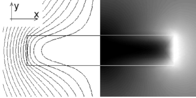
FIG. 1.: Right half: gray scale image of the magnetic field in and around the sample of $d/w=1/5$ and $\lambda/d=0.5$. Black color represents $B=0$. Left half: contour lines of the vector potential.

Consider an isotropic superconducting slab of width $2w$ in the $x$-direction, thickness $2d$ in the $y$-direction, and infinite in $z-$ direction. A uniform magnetic field $H_{0}$ is applied along the $y$ - direction. In this $2D$ geometry the vector potential is ${\bf A}=\{0,0,A\}$, so that the magnetic field has only two components ${\bf H}=\{\partial A/\partial y,-\partial A/\partial x,0\}$ and the London equation takes the form: $\Delta A-\lambda^{-2}A=0$. Outside the sample $\Delta A=-4\pi j/c=0$ and $\partial A/\partial n$ is continuous along the sample boundary. Here $n$ is the direction normal to the sample surface. A numerical solution of this equation was obtained using the finite-element method on a triangular adaptive mesh using Gauss-Newton iterations scheme. The boundary conditions were chosen to obtain constant magnetic field far from the sample, i.e., $A\left(x,y\right)=-H_{0}x$ for $y>>d$ and $x$ $>>w$.

Figure 1 presents the distribution of the the magnetic field in and around the sample with $w/d=5$ and $\lambda/d=0.5$. The black color on a gray scale image corresponds to $\left|{\bf B}\right|=0$. The left half of the sample shows contour lines of the vector potential. Figure 2 shows profiles of the y-component of the magnetic field at different distances $y$ from the sample middle plane.

FIG. 2.: Profiles of the y-component of the magnetic field (parallel to the external field) for the sample shown in Fig. 1. Inset corresponding profiles of the vector potential.

The inset shows the corresponding profiles of the vector potential, normalized by its value $A^{0}(x=w)$ in the absence of a sample (a uniform-field curve $A^{0}=x$ is shown by the dotted line). Using the London relation $4\pi\lambda^{2}j=-cA$ and the definition of the magnetic moment $M=(2c)^{-1}\int{\bf r}\times{\bf j}d^{3}r$ we calculate numerically the susceptibility per unit volume (unit of surface cross-section in 2D case):

$$4\pi\chi=\frac{1}{dw\lambda^{2}H_{0}}\int\limits_{0}^{d}dy\int\limits_{0}^{w}A\left(x,y\right)xdx$$ (1)

It is easy to check that for an infinite slab of width $2w$ in parallel field, where $A=-\lambda H_{0}\sinh{(x/\lambda)}/\cosh{(w/\lambda)}$, Eq.(1) results in a known expression similar to Eq.(4) below (with $N=0$ and $R=w$). In finite geometry there will be a contribution to the total susceptibility from the currents flowing on top and bottom surfaces. These currents are due to shielding of the in-plane component of the magnetic field, $H_{x}=\partial A/\partial y$, appearing due to demagnetization. Figure 3 shows profiles of $H_{x}$ on the sample surface, at $y=d$, calculated for three different samples, $w/d=$ 8, 5, and 2.5. An analytical form for the surface magnetic field is known only for elliptical samples. We find, however, that it can be mapped onto the flat surface, so that the distribution of $H_{x}$ is given by:

$$H_{x}=\frac{H_{0}r}{\sqrt{a^{2}-r^{2}}}$$ (2)

where $r\equiv x/w$ and $a^{2}=1+(2d/w)^{2}$. This equation is similar to that obtained for an ideal Meissner screening [5, 6]. Solid lines in Fig.3 are the fits to Eq.(2). The agreement between numerical and analytical results is apparent.

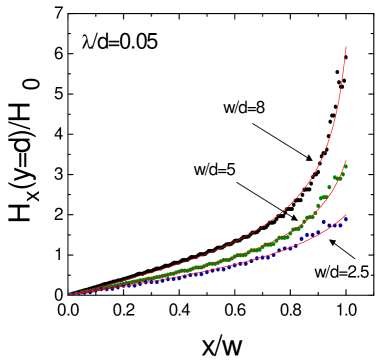
FIG. 3.: Distribution of the in-plane, $H_{x}$, component of the magnetic field on the sample surface, $y=d$. Symbols show result of numerical calculation and solid lines are the fits to Eq.(2).

Next we find a simple analytical approximation to the exact numerical results by calculating the ratio of the volume penetrated by the magnetic field to the total sample volume. This procedure automatically takes into account demagnetization and non-uniform distribution of the magnetic field along sample top and bottom faces. The exact calculation requires knowledge of $A(x,y)$ inside the sample or ${\bf H}(x,y)$ in a screened volume outside, proportional to $w^{2}$. The penetrated volume is:

$$V_{p}=\oint\limits_{S}{\frac{\lambda\left|{H_{s}}\right|}{H_{0}}ds}$$ (3)

where integration is conducted over the sample surface in a $3D$ case or sample cross-section perimeter in a $2D$ case. Using Eq.(2) for magnetic field on top and bottom surfaces and assuming $H_{s}=H_{0}/(1-N)$ on sides we obtain:

$$-4\pi\chi=\frac{1}{\left(1-N\right)}\left[1-\frac{\lambda}{R}\tanh\left(\frac{R}{\lambda}\right)\right]$$ (4)

Here $N$ is an effective demagnetization factor and $R$ is the effective dimension. Both depend on the dimensionality of the problem. As mentioned earlier, Eq.(4) is similar to the well-known solution for the infinite slab of width $2w$ in parallel field. In that case $R=w$ and the effective demagnetizing factor $N=0$. In a 3D case ($2w\times 2w$ slab, infinite in the $z-$ direction), $R=w/2$ and $N=0$. The $\tanh{(R/\lambda)}$ term in Eq. (4)was inserted to insure a correct limit at $\lambda\rightarrow\infty$. This correction becomes relevant at $\lambda/R\geq 0.4$, which is realized only at about $T/T_{c}\geq 0.9$ for typical high-$T_{c}$ samples.

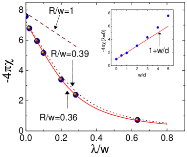
FIG. 4.: Calculated $-4\pi\chi\left(\lambda\right)$ for a slab of $w/d=5$. Solid line is a fit to Eq.(4) with the effective dimension $R/w=0.36$. Dotted line is calculated using $R/w=0.39$ from Eq.(5) and a dashed line is a plot with $R/w=1$. Inset: $-4\pi\chi\left(\lambda\rightarrow 0\right)$ calculated for samples of different aspect ratio. Solid line is $1+w/d$.

For the actual geometry studied here, both $R$ and $N$ depend upon the aspect ratio $w/d$. Unlike the case of an elliptical cross-section, the magnetic field is not constant within the sample so there is no true demagnetizing factor for a slab. However, $N$ can still be defined in the limit of $\lambda\rightarrow 0$, through the relation, $4\pi M/V_{s}=-H/\left(1-N\right)$. We find numerically that in a 2D case, for not too large aspect ratio $w/d$, $1/(1-N)\approx 1+w/d$. Calculating the expelled volume as described above, the effective dimension $R$ is given by:

$$R_{2D}=\frac{w}{1+\arcsin{(a^{-1})}}$$ (5)

In the thin limit, $d\ll w$ ($a\rightarrow 1$), we obtain $R_{2D}\approx 0.39w$.

The natural extension of this approach for the 3D disk of radius $w$ and thickness $2d$ leads to $1/(1-N)\approx 1+w/2d$ and

$$R_{3D}=\frac{w}{2\left(1+\left[1+(\frac{2d}{w})^{2}\right]\arctan{(\frac{w}{2d})}-\frac{2d}{w}\right)}$$ (6)

In a thin limit, $R_{3D}\approx 0.2w$. Eq.(6) was derived for a disk but the more experimentally relevant geometry is a rectangular slab. There is no analytical solution for the slab. However, $a^{2}=1+(2d/w)^{2}$ is relatively insensitive to ${w}$ in the thin limit and so we approximate $w$ for a slab by the geometric mean of its two lateral dimensions. The validity of this approach will be determined shortly.

To verify Eqs.(4) and (5) we calculated $\chi\left(\lambda\right)$ numerically. The result is shown it in Fig. 4 by symbols. The solid line is a fit to Eq.(4) with $N=0.86$ and $R/w=0.36$. The effective dimension calculated using Eq. (5) gives $R/w=0.39$ and the corresponding susceptibility curve is shown as a dotted line. The calculated effective demagnetization factor is $N=0.84$. It is seen that our approximations are reasonably good. It should be borne in mind that these are all $2D$ results - the sample extends to infinity in the z-direction. Demagnetizing effects are significantly larger in two dimensions than in three owing to the much slower decay of fields as we move away from the sample (compare $3D$ sphere, $N=1/3$, and cylinder in perpendicular field, $N=1/2$). Therefore we expect our approximations to work better in three dimensions.

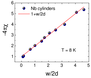
FIG. 5.: Linear magnetic susceptibility of Nb cylinders of different aspect ratio measured at $T=8$ K. Solid line is a plot of $1+w/2d$

In a 3D case the validity of our results can be verified experimentally by independently measuring the demagnetization factor as a function of the aspect ratio and the magnetic susceptibility for a finite London penetration depth $\lambda$. To achieve the first goal, we measured niobium cylinders of radius $w$ and length $2d$ using a Quantum Design MPMS-5 SQUID magnetometer. Sample dimensions were typically of the order of millimeters, which allows us to disregard London penetration depth of Nb (about 500 Å). The initial susceptibility obtained from the magnetization loops at $T=8$ K is shown in Fig. 5. The solid line is a plot of $1+w/2d$ (not the fit) and for an aspect ratio up to $w/d=10$ the agreement is excellent.

To test our result for $R$ (Eq.6) in actual samples we need the magnetic penetration depth. It is common to measure changes in the penetration depth by using the frequency shift of a microwave cavity or an LC resonator. In these techniques, the relative frequency shift $\left(f-f_{0}\right)/f_{0}$ due to a superconducting sample is proportional to $H^{-2}\int{{\bf M}_{ac}\cdot{\bf H}}dV$, which in turn is proportional to the sample linear magnetic susceptibility (${\bf M}_{ac}$ is the ac component of the total magnetic moment, ${\bf H}$ is the external magnetic field and $f_{0}$ is the resonance frequency in the absence of a sample). Using Eq.(4) and Eq.(6) we obtain for $\lambda<<R$:

$$\frac{\Delta f}{f_{0}}=\frac{V_{s}}{2V_{0}\left(1-N\right)}\left(1-\frac{\lambda}{R}\right)$$ (7)

where $V_{s}$ is the sample volume, $V_{0}$ is the effective coil volume. The apparatus and sample - dependent constant $\Delta f_{0}\equiv V_{s}f_{0}/(2V_{0}\left(1-N\right))$ is measured directly removing the sample from the coil. Thus, the change in $\lambda$ with respect to its value at low temperature is

$$\Delta\lambda=-\delta f\frac{R}{\Delta f_{0}}$$ (8)

where $\Delta\lambda\equiv\lambda\left(T\right)-\lambda\left(T_{\min}\right)$ and $\delta f\equiv\Delta f(T)-\Delta f(T_{min})$.

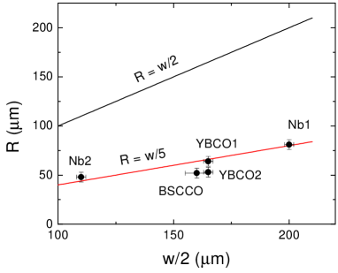
FIG. 6.: Effective dimension $R$ determined experimentally for different samples (symbols). The upper solid line is an ”infinite slab” model ($R=w/2$) and the lower solid line is an analytic approximation $R\approx w/5$.

We used an rf tunnel-diode resonator [7] to measure $\delta f$ in Nd foils, YBCO and BSCCO single crystals. Combining $\delta f$ with an independent measurement of $\Delta\lambda(T)$ and a measured value for $\Delta f_{0}$, we then arrived at an experimental determination of the effective dimension $R$. For the Nb and YBCO samples, $\Delta\lambda(T)$ was obtained using the demagnetization-free orientation (rf magnetic field along the sample $ab-$ plane) where $R=w$ and $1/(1-N)=1$. In BSCCO, the large anisotropy prohibits using this method and we used reported values of $d\lambda/dT\simeq$ 10 Å/K [8, 9]. Figure Fig. 6 summarizes our experimental results. The upper line represents the ”infinite slab” model, where $R=w/2$, whereas the lower solid line is $R=0.2w$ obtained in a thin limit of Eq. (6). Symbols show the experimental data obtained on different samples, indicated on plot. In three samples: YBCO1 (w/d = 57), Nb1 (w/d = 29) and Nb2 (w/d = 15), $R$ agrees with Eq.(6) to better than 5 %. The standard result, $R=w/2$, is too large by a factor of 2.5. Both YBCO2 and BSCCO give $R$ roughly 20 % smaller than predicted. For the BSCCO data, it is possible that a sample tilt combined with the very large anisotropy of $\lambda$ produces an additional contribution from $\lambda_{c}$. If the c-axis is tilted by an angle, $\theta$ away from the field direction, the frequency shift is given by

$$\frac{\Delta f}{f_{0}}=\frac{V_{s}}{2V_{0}\left(1-N\right)}\left({1-\frac{{\lambda_{ab}}}{R}}\right)\cos^{2}\left(\theta\right)+$$ (9)

$$\frac{V_{s}}{2V_{0}}\left({1-\left[{\frac{{\lambda_{ab}}}{d}+\frac{{\lambda_{c}}}{w}}\right]}\right)\sin^{2}\left(\theta\right)$$ (10)

The importance of the tilt depends upon the relative changes in $\lambda_{ab}$ and $\lambda_{c}$ with temperature. From Eq.(10) we obtain for the relative contribution to the frequency shift:

$$-\frac{{\delta f\left(\theta\right)}}{{\delta f\left({\theta=0}\right)}}\approx 1+\frac{2}{5}\tan^{2}\left(\theta\right)\left({1+\frac{d}{w}\frac{{\Delta\lambda_{c}}}{{\Delta\lambda_{ab}}}}\right)$$ (11)

where we used the previous estimates of $N$ and $R$. For BSCCO we take, $d\lambda_{c}/dT\simeq$ 170 Å/K and $d\lambda_{ab}/dT\simeq$ 10 Å/K [8, 9], Eq. (11) reduces to $\approx 1+\tan^{2}\left(\theta\right)$. We then find that for sample tilt to produce an additional 20 % frequency shift a misalignment of $\theta\approx 20^{o}$ would be required. Our estimated misalignment was a factor of 10 smaller than this so the discrepancy between measured and predicted R was not due to tilt. Both the BSCCO and the YBCO2 sample were more rectangular than square and our use of the geometric mean for $w$ could be the source of the error.

In conclusion, we solved numerically the London equations for samples of rectangular cross-section in perpendicular magnetic field. We obtained approximate formulae to estimate finite-$\lambda$ magnetic susceptibility of platelet samples (typical shape of high-$T_{c}$ superconducting crystals).

We thank M. V. Indenbom, E. H. Brandt, and J. R. Clem for useful discussions. This work was supported by Science and Technology Center for Superconductivity Grant No. NSF-DMR 91-20000. FMAM gratefully acknowledges Brazilian agencies FAPESP and CNPq for financial support.

REFERENCES

- [1] For example: J. F. Annett, N. D. Goldenfeld, and S. Renn, in Physical Properties of High Temperature Superconductors II, edited by D. M. Ginsberg (World Scientific, New Jersey, 1990).
- [2] E. H. Brandt, Phys. Rev. B 58, 6506 (1998); ibid, 6523;
- [3] M. W. Coffey, J. R. Clem, Phys. Rev. Lett. 67, 386 (1991); M. W. Coffey, J. R. Clem, Phys. Rev. B 45, 10527 (1992).
- [4] F. M. Araujo-Moreira et. al., Phys. Rev. B 61, 634 (2000).
- [5] W. T. Norris, J. of Physics D 3, 489 (1970).
- [6] P. Fabbricatore et. al., Phys. Rev. B, in print (2000).
- [7] C. T. Van Degrift Rev. Sci. Inst. 46, 599 (1975); A. Carrington et. al., Phys. Rev. B 59 (1999).
- [8] T. Jacobs et. al.,Phys. Rev. Lett. 75, 4516 (1995).
- [9] Shih-Fu Lee et. al. Phys. Rev. Lett. 77, 735 (1996); M. Nideröst et. al. Phys. Rev. Lett. 81, 3231 (1998).