Long-range interaction and nonlinear localized modes in photonic crystal waveguides

Abstract

We develop the theory of nonlinear localised modes (intrinsic localised modes or discrete breathers) in two-dimensional (2D) photonic crystal waveguides. We consider different geometries of the waveguides created by an array of nonlinear dielectric rods in an otherwise perfect linear 2D photonic crystal, and demonstrate that the effective interaction in such waveguides is nonlocal, being described by a new type of nonlinear lattice models with long-range coupling and nonlocal nonlinearity. We reveal the existence of different types of nonlinear guided modes which are also localised in the waveguide direction, and describe their unique properties including bistability.

I Introduction

In physics, the idea of localisation is generally associated with disorder that breaks translational invariance. However, research in recent years has demonstrated that localisation can occur in the absence of any disorder and solely due to nonlinearity, in the form of intrinsic localised modes, also called discrete breathers.[2] A rigorous proof of the existence of time-periodic, spatially localised solutions describing such nonlinear modes has been presented for a broad class of Hamiltonian coupled-oscillator nonlinear lattices,[3] but approximate analytical solutions can also be found in many other cases, demonstrating a generality of the concept of nonlinear localised modes.

Nonlinear localised modes can be easily identified in numerical molecular-dynamics simulations in many different physical models (see, e.g., Ref. [2] for a review), but only very recently the first experimental observations of spatially localised nonlinear modes have been reported in mixed-valence transition metal complexes,[4] quasi-one-dimensional antiferromagnetic chains,[5] and arrays of Josephson junctions.[6] Importantly, very similar types of spatially localised nonlinear modes have been experimentally observed in macroscopic mechanical [7] and guided-wave optical [8] systems.

Recent experimental observations of nonlinear localised modes, as well as numerous theoretical results, indicate that both effects, i.e. nonlinearity-induced localisation and spatially localised modes, can be expected in physical systems of very different nature. From the viewpoint of possible practical applications, self-localised states in optics seem to be the most promising ones; they can lead to different types of nonlinear all-optical switching devices where light manipulates and controls light itself, by varying the input intensity. As a result, the study of nonlinear localised modes in photonic structures is expected to bring a variety of realistic applications of intrinsic localised modes.

One of the promising fields where the concept of nonlinear localised modes may find practical applications is in the physics of photonic crystals [or photonic band gap (PBG) materials] — periodic dielectric structures that produce many of the same phenomena for photons as the crystalline atomic potential does for electrons.[9] Three-dimensional (3D) photonic crystals for visible light have been successfully fabricated only within the past year or two, and presently many research groups are working on creating tunable band-gap switches and transistors operating entirely with light. The most recent idea is to employ nonlinear properties of band-gap materials, thus creating nonlinear photonic crystals that have 2D or 3D periodic nonlinear susceptibility.[10, 11]

Nonlinear photonic crystals or photonic crystals with embedded nonlinear impurities create an ideal environment for the generation and observation of nonlinear localised photonic modes. In particular, such modes can be excited at nonlinear interfaces with quadratic nonlinearity,[12] or along dielectric waveguide structures possessing a nonlinear Kerr-type response.[13] In this paper, we analyse nonlinear localised modes in 2D photonic crystal waveguides. We consider the waveguides created by an array of dielectric rods in an otherwise perfect 2D photonic crystal. It is assumed that the dielectric constant of the waveguide rods depends on the field intensity (due to the Kerr effect), so that waveguides of different geometries can support a variety of nonlinear guided modes. We demonstrate here that localisation can occur in the propagation direction creating a 2D spatially localised mode (see Fig. 9 below). As follows from our results, the effective interaction in such nonlinear waveguides is nonlocal, and the nonlinear localised modes are described by a nontrivial generalisation of nonlinear lattice models with long-range coupling and nonlocal nonlinearity.

II Model

We consider a 2D photonic crystal created by a square lattice of parallel, infinitely long dielectric columns (or rods) in air. The system is characterized by the dielectric constant $\epsilon(\mathchoice{{\hbox{\boldmath$\displaystyle x$}}}{{\hbox{\boldmath$\textstyle x$}}}{{\hbox{\boldmath$\scriptstyle x$}}}{{\hbox{\boldmath$\scriptscriptstyle x$}}})=\epsilon(x_{1},x_{2})$, and it is assumed that the rods are parallel to the $x_{3}$ axis. The evolution of the TM-polarised [9] light [with the electric field having the structure $\mathchoice{{\hbox{\boldmath$\displaystyle E$}}}{{\hbox{\boldmath$\textstyle E$}}}{{\hbox{\boldmath$\scriptstyle E$}}}{{\hbox{\boldmath$\scriptscriptstyle E$}}}=(0,0,E)$], propagating in the $(x_{1},x_{2})$-plane, is governed by the scalar wave equation

$$\nabla^{2}E(\mathchoice{{\hbox{\boldmath$\displaystyle x$}}}{{\hbox{\boldmath$\textstyle x$}}}{{\hbox{\boldmath$\scriptstyle x$}}}{{\hbox{\boldmath$\scriptscriptstyle x$}}},t)-\frac{1}{c^{2}}\,\partial_{t}^{2}\left[\epsilon(\mathchoice{{\hbox{\boldmath$\displaystyle x$}}}{{\hbox{\boldmath$\textstyle x$}}}{{\hbox{\boldmath$\scriptstyle x$}}}{{\hbox{\boldmath$\scriptscriptstyle x$}}})E\right]=0\;,$$ (1)

where $\nabla^{2}\equiv\partial_{x_{1}}^{2}+\partial_{x_{2}}^{2}$. For monochromatic light, we consider the stationary solutions

$$E(\mathchoice{{\hbox{\boldmath$\displaystyle x$}}}{{\hbox{\boldmath$\textstyle x$}}}{{\hbox{\boldmath$\scriptstyle x$}}}{{\hbox{\boldmath$\scriptscriptstyle x$}}},t)=e^{-i\omega t}\,E(\mathchoice{{\hbox{\boldmath$\displaystyle x$}}}{{\hbox{\boldmath$\textstyle x$}}}{{\hbox{\boldmath$\scriptstyle x$}}}{{\hbox{\boldmath$\scriptscriptstyle x$}}}\,|\,\omega)\;,$$

and the equation of motion (1) reduces to the simple eigenvalue problem

$$\left[\nabla^{2}+\left(\frac{\omega}{c}\right)^{2}\epsilon(\mathchoice{{\hbox{\boldmath$\displaystyle x$}}}{{\hbox{\boldmath$\textstyle x$}}}{{\hbox{\boldmath$\scriptstyle x$}}}{{\hbox{\boldmath$\scriptscriptstyle x$}}})\right]E(\mathchoice{{\hbox{\boldmath$\displaystyle x$}}}{{\hbox{\boldmath$\textstyle x$}}}{{\hbox{\boldmath$\scriptstyle x$}}}{{\hbox{\boldmath$\scriptscriptstyle x$}}}\,|\,\omega)=0\;.$$ (2)

This eigenvalue problem can be easily solved (e.g., by the plane waves method [14]) in the case of a perfect photonic crystal, for which the dielectric constant $\epsilon(\mathchoice{{\hbox{\boldmath$\displaystyle x$}}}{{\hbox{\boldmath$\textstyle x$}}}{{\hbox{\boldmath$\scriptstyle x$}}}{{\hbox{\boldmath$\scriptscriptstyle x$}}})\equiv\epsilon_{pc}(\mathchoice{{\hbox{\boldmath$\displaystyle x$}}}{{\hbox{\boldmath$\textstyle x$}}}{{\hbox{\boldmath$\scriptstyle x$}}}{{\hbox{\boldmath$\scriptscriptstyle x$}}})$ is a periodic function

$$\epsilon_{pc}(\mathchoice{{\hbox{\boldmath$\displaystyle x$}}}{{\hbox{\boldmath$\textstyle x$}}}{{\hbox{\boldmath$\scriptstyle x$}}}{{\hbox{\boldmath$\scriptscriptstyle x$}}}+\mathchoice{{\hbox{\boldmath$\displaystyle s$}}}{{\hbox{\boldmath$\textstyle s$}}}{{\hbox{\boldmath$\scriptstyle s$}}}{{\hbox{\boldmath$\scriptscriptstyle s$}}}_{ij})=\epsilon_{pc}(\mathchoice{{\hbox{\boldmath$\displaystyle x$}}}{{\hbox{\boldmath$\textstyle x$}}}{{\hbox{\boldmath$\scriptstyle x$}}}{{\hbox{\boldmath$\scriptscriptstyle x$}}})\;,$$ (3)

where $i$ and $j$ are arbitrary integer, and

$$\mathchoice{{\hbox{\boldmath$\displaystyle s$}}}{{\hbox{\boldmath$\textstyle s$}}}{{\hbox{\boldmath$\scriptstyle s$}}}{{\hbox{\boldmath$\scriptscriptstyle s$}}}_{ij}=i\,\mathchoice{{\hbox{\boldmath$\displaystyle a$}}}{{\hbox{\boldmath$\textstyle a$}}}{{\hbox{\boldmath$\scriptstyle a$}}}{{\hbox{\boldmath$\scriptscriptstyle a$}}}_{1}+j\,\mathchoice{{\hbox{\boldmath$\displaystyle a$}}}{{\hbox{\boldmath$\textstyle a$}}}{{\hbox{\boldmath$\scriptstyle a$}}}{{\hbox{\boldmath$\scriptscriptstyle a$}}}_{2}$$ (4)

is a linear combination of the primitive lattice vectors $\mathchoice{{\hbox{\boldmath$\displaystyle a$}}}{{\hbox{\boldmath$\textstyle a$}}}{{\hbox{\boldmath$\scriptstyle a$}}}{{\hbox{\boldmath$\scriptscriptstyle a$}}}_{1}$ and $\mathchoice{{\hbox{\boldmath$\displaystyle a$}}}{{\hbox{\boldmath$\textstyle a$}}}{{\hbox{\boldmath$\scriptstyle a$}}}{{\hbox{\boldmath$\scriptscriptstyle a$}}}_{2}$ of the 2D photonic crystal.

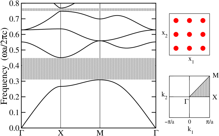
FIG. 1.: The band-gap structure of the photonic crystal consisting of a square lattice of dielectric rods with $r_{0}=0.18a$ and $\epsilon_{0}=11.56$ (the band gaps are shaded grey). The top right inset shows a cross-sectional view of the 2D photonic crystal. The bottom right inset shows the corresponding Brillouin zone, with the irreducible zone shaded grey.

For definiteness, we consider the 2D photonic crystal earlier analysed (in the linear limit) in Refs. [15, 16], i.e. we assume that the rods are identical and cylindrical, with radius $r_{0}=0.18a$ and dielectric constant $\epsilon_{0}=11.56$. The rods form a perfect square lattice with the distance $a$ between two neighbouring rods, i.e. $\mathchoice{{\hbox{\boldmath$\displaystyle a$}}}{{\hbox{\boldmath$\textstyle a$}}}{{\hbox{\boldmath$\scriptstyle a$}}}{{\hbox{\boldmath$\scriptscriptstyle a$}}}_{1}=a\mathchoice{{\hbox{\boldmath$\displaystyle x$}}}{{\hbox{\boldmath$\textstyle x$}}}{{\hbox{\boldmath$\scriptstyle x$}}}{{\hbox{\boldmath$\scriptscriptstyle x$}}}_{1}$ and $\mathchoice{{\hbox{\boldmath$\displaystyle a$}}}{{\hbox{\boldmath$\textstyle a$}}}{{\hbox{\boldmath$\scriptstyle a$}}}{{\hbox{\boldmath$\scriptscriptstyle a$}}}_{2}=a\mathchoice{{\hbox{\boldmath$\displaystyle x$}}}{{\hbox{\boldmath$\textstyle x$}}}{{\hbox{\boldmath$\scriptstyle x$}}}{{\hbox{\boldmath$\scriptscriptstyle x$}}}_{2}$. The frequency band structure for this type of 2D photonic crystal, and for the selected polarisations of the electric field, is shown in Fig. 1. As follows from the structure of the frequency spectrum, there exists a large (38%) band gap that extends from the lower cut-off frequency, $\omega=0.302\times 2\pi c/a$, to the upper band-gap frequency, $\omega=0.443\times 2\pi c/a$. Since the characteristics of a PBG material remain unchanged under rescaling, we can assume that this gap is created either in the infra-red or visible regions of the spectrum. For example, if we choose the lattice constant to be $a=0.58\,\mu$m, the wavelength corresponding to the mid-gap frequency will be $1.55\,\mu$m.

The TM-polarised light cannot propagate through the photonic crystal if its frequency falls inside the band gap. But one can excite guided modes inside the forbidden frequency gap by introducing some interfaces, waveguides, or defects. Here, we consider waveguides created by a row of identical defects with a Kerr-type nonlinear response. These defect-induced waveguides possess translational symmetry, and the corresponding guided modes can be characterized by the reciprocal space wave vector $k$ directed along the waveguide. Such a guided mode has a periodical profile inside the waveguide, and it decays exponentially outside it.

Linear photonic-crystal waveguides created by removing a row of dielectric rods have been recently investigated numerically [15, 16] and experimentally.[17] In particular, highly efficient transmission of light, even in the case of a bent waveguide, has been demonstrated.

In the present paper, in contrast to Refs. [15, 16, 17] where only linear waveguides were considered, we study the properties of nonlinear waveguides created by inserting an additional row of rods fabricated from a Kerr-type nonlinear material characterized by a third-order nonlinear susceptibility with the linear dielectric constant $\epsilon_{d}$. For definiteness, we assume that $\epsilon_{d}=\epsilon_{0}=11.56$. As we show below, changing the radius $r_{d}$ of these defect rods and their location within the crystal, we can create waveguides with quite different properties.

III Effective discrete equations

Writing the dielectric constant $\epsilon(\mathchoice{{\hbox{\boldmath$\displaystyle x$}}}{{\hbox{\boldmath$\textstyle x$}}}{{\hbox{\boldmath$\scriptstyle x$}}}{{\hbox{\boldmath$\scriptscriptstyle x$}}})$ as a sum of periodic and defect-induced terms, i.e.

$$\epsilon(\mathchoice{{\hbox{\boldmath$\displaystyle x$}}}{{\hbox{\boldmath$\textstyle x$}}}{{\hbox{\boldmath$\scriptstyle x$}}}{{\hbox{\boldmath$\scriptscriptstyle x$}}})=\epsilon_{pc}(\mathchoice{{\hbox{\boldmath$\displaystyle x$}}}{{\hbox{\boldmath$\textstyle x$}}}{{\hbox{\boldmath$\scriptstyle x$}}}{{\hbox{\boldmath$\scriptscriptstyle x$}}})+\delta\epsilon(\mathchoice{{\hbox{\boldmath$\displaystyle x$}}}{{\hbox{\boldmath$\textstyle x$}}}{{\hbox{\boldmath$\scriptstyle x$}}}{{\hbox{\boldmath$\scriptscriptstyle x$}}}\,|\,E)\;,$$

we can present Eq. (2) as follows,

$$\left[\nabla^{2}+\left(\frac{\omega}{c}\right)^{2}\epsilon_{pc}(\mathchoice{{\hbox{\boldmath$\displaystyle x$}}}{{\hbox{\boldmath$\textstyle x$}}}{{\hbox{\boldmath$\scriptstyle x$}}}{{\hbox{\boldmath$\scriptscriptstyle x$}}})\right] E(\mathchoice{{\hbox{\boldmath$\displaystyle x$}}}{{\hbox{\boldmath$\textstyle x$}}}{{\hbox{\boldmath$\scriptstyle x$}}}{{\hbox{\boldmath$\scriptscriptstyle x$}}}\,|\,\omega)$$ (5)

$$=- \left(\frac{\omega}{c}\right)^{2}\delta\epsilon(\mathchoice{{\hbox{\boldmath$\displaystyle x$}}}{{\hbox{\boldmath$\textstyle x$}}}{{\hbox{\boldmath$\scriptstyle x$}}}{{\hbox{\boldmath$\scriptscriptstyle x$}}}\,|\,E)\,E(\mathchoice{{\hbox{\boldmath$\displaystyle x$}}}{{\hbox{\boldmath$\textstyle x$}}}{{\hbox{\boldmath$\scriptstyle x$}}}{{\hbox{\boldmath$\scriptscriptstyle x$}}}\,|\,\omega)\;.$$ (6)

Equation (6) can also be written in the integral form

$$E(\mathchoice{{\hbox{\boldmath$\displaystyle x$}}}{{\hbox{\boldmath$\textstyle x$}}}{{\hbox{\boldmath$\scriptstyle x$}}}{{\hbox{\boldmath$\scriptscriptstyle x$}}}\,|\,\omega)=\left(\frac{\omega}{c}\right)^{2}\!\!\int d^{2}\mathchoice{{\hbox{\boldmath$\displaystyle y$}}}{{\hbox{\boldmath$\textstyle y$}}}{{\hbox{\boldmath$\scriptstyle y$}}}{{\hbox{\boldmath$\scriptscriptstyle y$}}}\,\,\,G(\mathchoice{{\hbox{\boldmath$\displaystyle x$}}}{{\hbox{\boldmath$\textstyle x$}}}{{\hbox{\boldmath$\scriptstyle x$}}}{{\hbox{\boldmath$\scriptscriptstyle x$}}},\mathchoice{{\hbox{\boldmath$\displaystyle y$}}}{{\hbox{\boldmath$\textstyle y$}}}{{\hbox{\boldmath$\scriptstyle y$}}}{{\hbox{\boldmath$\scriptscriptstyle y$}}}\,|\,\omega)\,\delta\epsilon(\mathchoice{{\hbox{\boldmath$\displaystyle y$}}}{{\hbox{\boldmath$\textstyle y$}}}{{\hbox{\boldmath$\scriptstyle y$}}}{{\hbox{\boldmath$\scriptscriptstyle y$}}}\,|\,E)\,E(\mathchoice{{\hbox{\boldmath$\displaystyle y$}}}{{\hbox{\boldmath$\textstyle y$}}}{{\hbox{\boldmath$\scriptstyle y$}}}{{\hbox{\boldmath$\scriptscriptstyle y$}}}\,|\,\omega)\;,$$ (7)

where $G(\mathchoice{{\hbox{\boldmath$\displaystyle x$}}}{{\hbox{\boldmath$\textstyle x$}}}{{\hbox{\boldmath$\scriptstyle x$}}}{{\hbox{\boldmath$\scriptscriptstyle x$}}},\mathchoice{{\hbox{\boldmath$\displaystyle y$}}}{{\hbox{\boldmath$\textstyle y$}}}{{\hbox{\boldmath$\scriptstyle y$}}}{{\hbox{\boldmath$\scriptscriptstyle y$}}}\,|\,\omega)$ is the Green function which is defined, in a standard way, as a solution of the equation

$$\left[\nabla^{2}+\left(\frac{\omega}{c}\right)^{2}\epsilon_{pc}(\mathchoice{{\hbox{\boldmath$\displaystyle x$}}}{{\hbox{\boldmath$\textstyle x$}}}{{\hbox{\boldmath$\scriptstyle x$}}}{{\hbox{\boldmath$\scriptscriptstyle x$}}})\right]G(\mathchoice{{\hbox{\boldmath$\displaystyle x$}}}{{\hbox{\boldmath$\textstyle x$}}}{{\hbox{\boldmath$\scriptstyle x$}}}{{\hbox{\boldmath$\scriptscriptstyle x$}}},\mathchoice{{\hbox{\boldmath$\displaystyle y$}}}{{\hbox{\boldmath$\textstyle y$}}}{{\hbox{\boldmath$\scriptstyle y$}}}{{\hbox{\boldmath$\scriptscriptstyle y$}}}\,|\,\omega)=-\delta(\mathchoice{{\hbox{\boldmath$\displaystyle x$}}}{{\hbox{\boldmath$\textstyle x$}}}{{\hbox{\boldmath$\scriptstyle x$}}}{{\hbox{\boldmath$\scriptscriptstyle x$}}}-\mathchoice{{\hbox{\boldmath$\displaystyle y$}}}{{\hbox{\boldmath$\textstyle y$}}}{{\hbox{\boldmath$\scriptstyle y$}}}{{\hbox{\boldmath$\scriptscriptstyle y$}}})\;,$$

with, accordingly to Eq. (3), periodic coefficients. The properties of the Green function and the numerical methods for its calculation have been already described in the literature. [14, 18] Here, we notice that the Green function of a perfect 2D photonic crystal is symmetric, i.e.

$$G(\mathchoice{{\hbox{\boldmath$\displaystyle x$}}}{{\hbox{\boldmath$\textstyle x$}}}{{\hbox{\boldmath$\scriptstyle x$}}}{{\hbox{\boldmath$\scriptscriptstyle x$}}},\mathchoice{{\hbox{\boldmath$\displaystyle y$}}}{{\hbox{\boldmath$\textstyle y$}}}{{\hbox{\boldmath$\scriptstyle y$}}}{{\hbox{\boldmath$\scriptscriptstyle y$}}}\,|\,\omega)=G(\mathchoice{{\hbox{\boldmath$\displaystyle y$}}}{{\hbox{\boldmath$\textstyle y$}}}{{\hbox{\boldmath$\scriptstyle y$}}}{{\hbox{\boldmath$\scriptscriptstyle y$}}},\mathchoice{{\hbox{\boldmath$\displaystyle x$}}}{{\hbox{\boldmath$\textstyle x$}}}{{\hbox{\boldmath$\scriptstyle x$}}}{{\hbox{\boldmath$\scriptscriptstyle x$}}}\,|\,\omega)$$

and periodic, i.e.

$$G(\mathchoice{{\hbox{\boldmath$\displaystyle x$}}}{{\hbox{\boldmath$\textstyle x$}}}{{\hbox{\boldmath$\scriptstyle x$}}}{{\hbox{\boldmath$\scriptscriptstyle x$}}}+\mathchoice{{\hbox{\boldmath$\displaystyle s$}}}{{\hbox{\boldmath$\textstyle s$}}}{{\hbox{\boldmath$\scriptstyle s$}}}{{\hbox{\boldmath$\scriptscriptstyle s$}}}_{ij},\mathchoice{{\hbox{\boldmath$\displaystyle y$}}}{{\hbox{\boldmath$\textstyle y$}}}{{\hbox{\boldmath$\scriptstyle y$}}}{{\hbox{\boldmath$\scriptscriptstyle y$}}}+\mathchoice{{\hbox{\boldmath$\displaystyle s$}}}{{\hbox{\boldmath$\textstyle s$}}}{{\hbox{\boldmath$\scriptstyle s$}}}{{\hbox{\boldmath$\scriptscriptstyle s$}}}_{ij}\,|\,\omega)=G(\mathchoice{{\hbox{\boldmath$\displaystyle x$}}}{{\hbox{\boldmath$\textstyle x$}}}{{\hbox{\boldmath$\scriptstyle x$}}}{{\hbox{\boldmath$\scriptscriptstyle x$}}},\mathchoice{{\hbox{\boldmath$\displaystyle y$}}}{{\hbox{\boldmath$\textstyle y$}}}{{\hbox{\boldmath$\scriptstyle y$}}}{{\hbox{\boldmath$\scriptscriptstyle y$}}}\,|\,\omega)\;,$$

where $\mathchoice{{\hbox{\boldmath$\displaystyle s$}}}{{\hbox{\boldmath$\textstyle s$}}}{{\hbox{\boldmath$\scriptstyle s$}}}{{\hbox{\boldmath$\scriptscriptstyle s$}}}_{ij}$ is defined by Eq. (4).

Let us consider a row of nonlinear defect rods embedded into the crystal along a selected direction. To describe such a row, we should define the rods positions along $\mathchoice{{\hbox{\boldmath$\displaystyle s$}}}{{\hbox{\boldmath$\textstyle s$}}}{{\hbox{\boldmath$\scriptstyle s$}}}{{\hbox{\boldmath$\scriptscriptstyle s$}}}_{ij}$ with some specific values of $i$ and $j$. For example, let us first assume that the defect rods are located at the points $\mathchoice{{\hbox{\boldmath$\displaystyle x$}}}{{\hbox{\boldmath$\textstyle x$}}}{{\hbox{\boldmath$\scriptstyle x$}}}{{\hbox{\boldmath$\scriptscriptstyle x$}}}_{m}=\mathchoice{{\hbox{\boldmath$\displaystyle x$}}}{{\hbox{\boldmath$\textstyle x$}}}{{\hbox{\boldmath$\scriptstyle x$}}}{{\hbox{\boldmath$\scriptscriptstyle x$}}}_{0}+m\,\mathchoice{{\hbox{\boldmath$\displaystyle s$}}}{{\hbox{\boldmath$\textstyle s$}}}{{\hbox{\boldmath$\scriptstyle s$}}}{{\hbox{\boldmath$\scriptscriptstyle s$}}}_{ij}$. In this case, the correction to the dielectric constant is

$$\delta\epsilon(\mathchoice{{\hbox{\boldmath$\displaystyle x$}}}{{\hbox{\boldmath$\textstyle x$}}}{{\hbox{\boldmath$\scriptstyle x$}}}{{\hbox{\boldmath$\scriptscriptstyle x$}}})=\left\{\epsilon_{d}+|E(\mathchoice{{\hbox{\boldmath$\displaystyle x$}}}{{\hbox{\boldmath$\textstyle x$}}}{{\hbox{\boldmath$\scriptstyle x$}}}{{\hbox{\boldmath$\scriptscriptstyle x$}}}\,|\,\omega)|^{2}\right\}\sum_{m}\theta(\mathchoice{{\hbox{\boldmath$\displaystyle x$}}}{{\hbox{\boldmath$\textstyle x$}}}{{\hbox{\boldmath$\scriptstyle x$}}}{{\hbox{\boldmath$\scriptscriptstyle x$}}}-\mathchoice{{\hbox{\boldmath$\displaystyle x$}}}{{\hbox{\boldmath$\textstyle x$}}}{{\hbox{\boldmath$\scriptstyle x$}}}{{\hbox{\boldmath$\scriptscriptstyle x$}}}_{m})\;,$$ (8)

where

$$\theta(\mathchoice{{\hbox{\boldmath$\displaystyle x$}}}{{\hbox{\boldmath$\textstyle x$}}}{{\hbox{\boldmath$\scriptstyle x$}}}{{\hbox{\boldmath$\scriptscriptstyle x$}}})=\left\{\begin{array}[]{c}1\;,\quad\mbox{for}\quad|\mathchoice{{\hbox{\boldmath$\displaystyle x$}}}{{\hbox{\boldmath$\textstyle x$}}}{{\hbox{\boldmath$\scriptstyle x$}}}{{\hbox{\boldmath$\scriptscriptstyle x$}}}|\leq r_{d}\;,\\ 0\;,\quad\mbox{for}\quad|\mathchoice{{\hbox{\boldmath$\displaystyle x$}}}{{\hbox{\boldmath$\textstyle x$}}}{{\hbox{\boldmath$\scriptstyle x$}}}{{\hbox{\boldmath$\scriptscriptstyle x$}}}|>r_{d}\;.\end{array}\right.$$

Assuming that the radius of the rods, $r_{d}$, is sufficiently small (so that the electric field $E(\mathchoice{{\hbox{\boldmath$\displaystyle x$}}}{{\hbox{\boldmath$\textstyle x$}}}{{\hbox{\boldmath$\scriptstyle x$}}}{{\hbox{\boldmath$\scriptscriptstyle x$}}}\,|\,\omega)$ is almost constant inside the defect rods), we substitute Eq. (8) into Eq. (7) and, averaging over of the cross-section of the rods, derive an approximate discrete nonlinear equation for the electric field

$$E_{n}=\sum_{m}J_{n-m}(\omega)(\epsilon_{d}+|E_{m}|^{2})E_{m}\;,$$ (9)

where

$$J_{n}(\omega)=\left(\frac{\omega}{c}\right)^{2}\int\limits_{r_{d}}d^{2}\mathchoice{{\hbox{\boldmath$\displaystyle y$}}}{{\hbox{\boldmath$\textstyle y$}}}{{\hbox{\boldmath$\scriptstyle y$}}}{{\hbox{\boldmath$\scriptscriptstyle y$}}}\,\,\,G(\mathchoice{{\hbox{\boldmath$\displaystyle x$}}}{{\hbox{\boldmath$\textstyle x$}}}{{\hbox{\boldmath$\scriptstyle x$}}}{{\hbox{\boldmath$\scriptscriptstyle x$}}}_{0},\mathchoice{{\hbox{\boldmath$\displaystyle x$}}}{{\hbox{\boldmath$\textstyle x$}}}{{\hbox{\boldmath$\scriptstyle x$}}}{{\hbox{\boldmath$\scriptscriptstyle x$}}}_{n}+\mathchoice{{\hbox{\boldmath$\displaystyle y$}}}{{\hbox{\boldmath$\textstyle y$}}}{{\hbox{\boldmath$\scriptstyle y$}}}{{\hbox{\boldmath$\scriptscriptstyle y$}}}\,|\,\omega)\;.$$ (10)

This type of discrete nonlinear equation for photonic crystals has been earlier introduced by McGurn [13], for the special case of nonlinear impurities embedded in the linear rods. However, the analytical approach developed by McGurn for that model did not take into account the field distribution via the explicit dependence of the coupling coefficients $J_{n}(\omega)$ and, as a result, the equation (9) was not solved exactly. Moreover, the analysis of Ref. [13] was based on the nearest-neighbour approximation where the coupling coefficients are approximated as $J_{n}=J_{0}\delta_{n,0}+J_{1}\delta_{n,\pm 1}$ with constant $J_{0}$ and $J_{1}$.

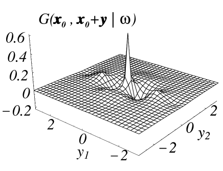
FIG. 2.: The Green function $G(\mathchoice{{\hbox{\boldmath$\displaystyle x$}}}{{\hbox{\boldmath$\textstyle x$}}}{{\hbox{\boldmath$\scriptstyle x$}}}{{\hbox{\boldmath$\scriptscriptstyle x$}}}_{0},\mathchoice{{\hbox{\boldmath$\displaystyle x$}}}{{\hbox{\boldmath$\textstyle x$}}}{{\hbox{\boldmath$\scriptstyle x$}}}{{\hbox{\boldmath$\scriptscriptstyle x$}}}_{0}+\mathchoice{{\hbox{\boldmath$\displaystyle y$}}}{{\hbox{\boldmath$\textstyle y$}}}{{\hbox{\boldmath$\scriptstyle y$}}}{{\hbox{\boldmath$\scriptscriptstyle y$}}}\,|\,\omega)$ for $\mathchoice{{\hbox{\boldmath$\displaystyle x$}}}{{\hbox{\boldmath$\textstyle x$}}}{{\hbox{\boldmath$\scriptstyle x$}}}{{\hbox{\boldmath$\scriptscriptstyle x$}}}_{0}=\mathchoice{{\hbox{\boldmath$\displaystyle a$}}}{{\hbox{\boldmath$\textstyle a$}}}{{\hbox{\boldmath$\scriptstyle a$}}}{{\hbox{\boldmath$\scriptscriptstyle a$}}}_{1}/2$ and $\omega=0.33\times 2\pi c/a$.

In a sharp contrast, in the present paper we provide a systematic numerical analysis of different types of nonlinear localised modes in the framework of a complete model. In particular, we reveal that the approximation of the nearest-neighbour interaction is very crude in many of the cases analysed. Since the effective coupling coefficients are defined by the Green function, this can be seen directly from Fig. 2 that shows a typical spatial profile of the Green function which, in general, characterises a long-range interaction, very typical for photonic crystal waveguides. As a consequence of that, the coupling coefficients $|J_{n}(\omega)|$ calculated from Eq. (10) decrease exponentially with the site number $n$, and in the asymptotic region they can be presented as follows

$$|J_{n}(\omega)|\approx\left\{\begin{array}[]{lcc}J_{0}(\omega)\;,&\mbox{for}&n=0\;,\\ J_{*}(\omega)\,e^{-\alpha(\omega)|n|}\;,&\mbox{for}&|n|\geq 1\;,\end{array}\right.$$

where the characteristic decay rate $\alpha(\omega)$ can be as small as $0.85$, depending on the values of $\omega$, $\mathchoice{{\hbox{\boldmath$\displaystyle x$}}}{{\hbox{\boldmath$\textstyle x$}}}{{\hbox{\boldmath$\scriptstyle x$}}}{{\hbox{\boldmath$\scriptscriptstyle x$}}}_{0}$, $\mathchoice{{\hbox{\boldmath$\displaystyle s$}}}{{\hbox{\boldmath$\textstyle s$}}}{{\hbox{\boldmath$\scriptstyle s$}}}{{\hbox{\boldmath$\scriptscriptstyle s$}}}_{ij}$, and $r_{d}$, and it can be even smaller for other types of photonic crystals.

This result allows us to draw an analogy with a class of the nonlinear Schrödinger (NLS) equations that describe nonlinear excitations in quasi-one-dimensional molecular chains with long-range (e.g. dipole-dipole) interaction between the particles and local on-site nonlinearities.[19] For such systems, it was shown that the effect of nonlocal interparticle interaction introduces some new features in the properties of existence and stability of nonlinear localised modes. Moreover, for our model the coupling coefficients $J_{n}(\omega)$ can be either non-staggered and monotonically decaying, i.e. $J_{n}(\omega)=|J_{n}(\omega)|$, or staggered and oscillating from site to site, i.e. $J_{n}(\omega)=(-1)^{n}|J_{n}(\omega)|$. We can therefore expect that effective nonlocality in both linear and nonlinear terms of Eq. (9) will bring a number of new features in the properties of nonlinear localised modes.

IV Examples of nonlinear modes

As can be seen from the structure of the example Green function, presented in Fig. 2, the case of monotonically varying $J_{n}(\omega)$ can be obtained by locating the defect rods at the points $\mathchoice{{\hbox{\boldmath$\displaystyle x$}}}{{\hbox{\boldmath$\textstyle x$}}}{{\hbox{\boldmath$\scriptstyle x$}}}{{\hbox{\boldmath$\scriptscriptstyle x$}}}_{0}=\mathchoice{{\hbox{\boldmath$\displaystyle a$}}}{{\hbox{\boldmath$\textstyle a$}}}{{\hbox{\boldmath$\scriptstyle a$}}}{{\hbox{\boldmath$\scriptscriptstyle a$}}}_{1}/2$, along the straight line in the $\mathchoice{{\hbox{\boldmath$\displaystyle s$}}}{{\hbox{\boldmath$\textstyle s$}}}{{\hbox{\boldmath$\scriptstyle s$}}}{{\hbox{\boldmath$\scriptscriptstyle s$}}}_{01}$ direction. In this case, the frequency of a linear guided mode, that can be excited in such a waveguide, takes the minimum value at $k=0$ (see Fig. 3), and the corresponding nonlinear mode is expected to be non-staggered.

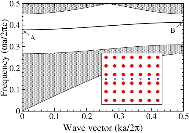
FIG. 3.: Dispersion relation for the photonic crystal waveguide shown in the inset ($\epsilon_{0}=\epsilon_{d}=11.56$, $r_{0}=0.18a$, $r_{d}=0.10a$). The grey areas are the projected band structure of the perfect 2D photonic crystal. The frequencies at the indicated points are: $\omega_{A}=0.378\times 2\pi c/a$ and $\omega_{B}=0.412\times 2\pi c/a$.

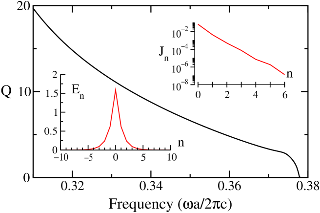
FIG. 4.: Intensity $Q(\omega)$ of the nonlinear mode excited in the photonic crystal waveguide shown in Fig. 3. The right inset gives the dependence $J_{n}(\omega)$ calculated at $\omega=0.37\times 2\pi c/a$. The left inset presents the profile of the corresponding nonlinear localised mode.

We have solved Eq. (9) numerically and found that nonlinearity can lead to the existence of a new type of guided modes which are localised in both directions, i.e. in the direction perpendicular to the waveguide, due to the guiding properties of a channel created by defect rods, and in the direction of the waveguide, due to the self-trapping effect. Such nonlinear modes exist with frequencies below the frequency of the linear guided mode of the waveguide, i.e. below the frequency $\omega_{A}$ in Fig. 3, and are indeed non-staggered, with the bell-shaped profile along the waveguide direction shown in the left inset of Fig. 4.

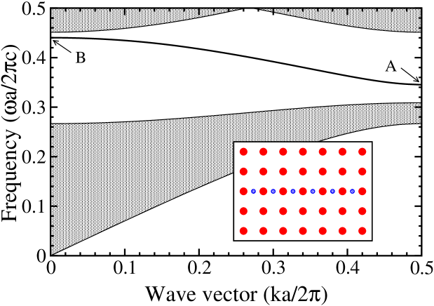
FIG. 5.: Dispersion relation for the photonic crystal waveguide shown in the inset ($\epsilon_{0}=\epsilon_{d}=11.56$, $r_{0}=0.18a$, $r_{d}=0.10a$). The grey areas are the projected band structure of the perfect 2D photonic crystal. The frequencies at the indicated points are: $\omega_{A}=0.346\times 2\pi c/a$ and $\omega_{B}=0.440\times 2\pi c/a$.

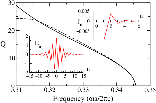
FIG. 6.: Intensity $Q(\omega)$ of the nonlinear mode excited in the photonic crystal waveguide shown in Fig. 5. The solid curve corresponds to the case of nonlinear rods in a linear photonic crystal, whereas the dashed curve is the same dependence for the case of a nonlinear photonic crystal. The right inset shows the behaviour of the coupling coefficients $J_{n}(\omega)$ for $n\geq 1$ ($J_{0}=0.045$) at $\omega=0.33\times 2\pi c/a$. The left inset shows the profile of the corresponding nonlinear mode.

The 2D nonlinear modes localised in both dimensions can be characterized by the mode intensity which we define, by analogy with the NLS equation, as

$$Q=\sum_{n}|E_{n}|^{2}.$$ (11)

This intensity is closely related to the energy of the electric field in the 2D photonic crystal accumulated in the nonlinear mode. In Fig. 4 we plot the dependence of $Q$ on frequency, for the waveguide geometry shown in Fig. 3.

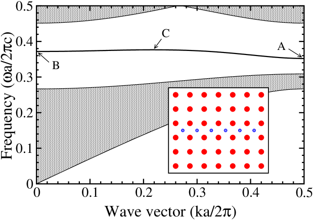
FIG. 7.: Dispersion relation for the photonic crystal waveguide shown in the inset ($\epsilon_{0}=\epsilon_{d}=11.56$, $r_{0}=0.18a$, $r_{d}=0.10a$). The grey areas are the projected band structure of the perfect crystal. The frequencies at the points indicated are: $\omega_{A}=0.352\times 2\pi c/a$, $\omega_{B}=0.371\times 2\pi c/a$, and $\omega_{C}=0.376\times 2\pi c/a$ (at $k=0.217\times 2\pi/a$).

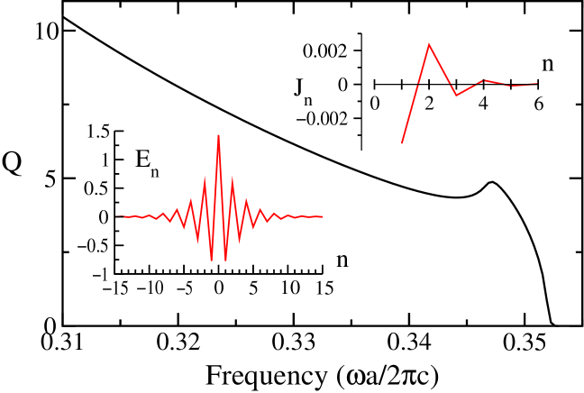
FIG. 8.: Intensity $Q(\omega)$ of the nonlinear mode excited in the photonic crystal waveguide shown in Fig. 7. The right inset shows the behaviour of the coupling coefficients $J_{n}(\omega)$ for $n\geq 1$ ($J_{0}=0.068$) at $\omega=0.345\times 2\pi c/a$. The left inset shows the profile of the corresponding nonlinear mode.

As can be seen from the example of the Green function shown in Fig. 2, the case of staggered coupling coefficients $J_{n}(\omega)$ can be obtained by locating the defect rods at the points $\mathchoice{{\hbox{\boldmath$\displaystyle x$}}}{{\hbox{\boldmath$\textstyle x$}}}{{\hbox{\boldmath$\scriptstyle x$}}}{{\hbox{\boldmath$\scriptscriptstyle x$}}}_{0}=\mathchoice{{\hbox{\boldmath$\displaystyle a$}}}{{\hbox{\boldmath$\textstyle a$}}}{{\hbox{\boldmath$\scriptstyle a$}}}{{\hbox{\boldmath$\scriptscriptstyle a$}}}_{1}/2$, along the straight line in the $\mathchoice{{\hbox{\boldmath$\displaystyle s$}}}{{\hbox{\boldmath$\textstyle s$}}}{{\hbox{\boldmath$\scriptstyle s$}}}{{\hbox{\boldmath$\scriptscriptstyle s$}}}_{10}$ direction. In this case, the frequency dependence of the linear guided mode of the waveguide takes the minimum at $k=\pi/a$ (see Fig. 5). Accordingly, the nonlinear guided mode localised along the direction of the waveguide is expected to exist with the frequency below the lowest frequency $\omega_{A}$ of the linear guided mode, with a staggered profile. The longitudinal profile of such a 2D nonlinear localised mode is shown in the left inset in Fig. 6, together with the dependence of the mode intensity $Q$ on the frequency (solid curve), which in this case is again monotonic.

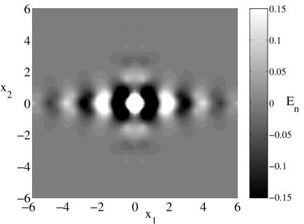
FIG. 9.: Contour plot of the the nonlinear localised mode that corresponds to the longitudinal cross-section shown in the left inset of Fig. 8.

The results presented above are obtained for linear photonic crystals with nonlinear waveguides created by a row of defect rods. However, we have carried out the same analysis for the general case of a nonlinear photonic crystal that is created by rods of different size but made of the same nonlinear material. Importantly, we have found very small difference in all the results for relatively weak nonlinearities. In particular, for the photonic crystal waveguide shown in Fig. 5, the results for linear and nonlinear photonic crystals are very close. Indeed, for the mode intensity $Q$ the results corresponding to a nonlinear photonic crystal are shown in Fig. 6 by a dashed curve, and for $Q<20$ this curve almost coincides with the solid curve corresponding to the case of a nonlinear waveguide embedded into a linear photonic crystal.

Let us now consider the waveguide created by a row of defects which are located at the points $\mathchoice{{\hbox{\boldmath$\displaystyle x$}}}{{\hbox{\boldmath$\textstyle x$}}}{{\hbox{\boldmath$\scriptstyle x$}}}{{\hbox{\boldmath$\scriptscriptstyle x$}}}_{0}=(\mathchoice{{\hbox{\boldmath$\displaystyle a$}}}{{\hbox{\boldmath$\textstyle a$}}}{{\hbox{\boldmath$\scriptstyle a$}}}{{\hbox{\boldmath$\scriptscriptstyle a$}}}_{1}+\mathchoice{{\hbox{\boldmath$\displaystyle a$}}}{{\hbox{\boldmath$\textstyle a$}}}{{\hbox{\boldmath$\scriptstyle a$}}}{{\hbox{\boldmath$\scriptscriptstyle a$}}}_{2})/2$, along a straight line in either the $\mathchoice{{\hbox{\boldmath$\displaystyle s$}}}{{\hbox{\boldmath$\textstyle s$}}}{{\hbox{\boldmath$\scriptstyle s$}}}{{\hbox{\boldmath$\scriptscriptstyle s$}}}_{10}$ or $\mathchoice{{\hbox{\boldmath$\displaystyle s$}}}{{\hbox{\boldmath$\textstyle s$}}}{{\hbox{\boldmath$\scriptstyle s$}}}{{\hbox{\boldmath$\scriptscriptstyle s$}}}_{01}$ directions. The results for this case are presented in Figs. 7–9. The coupling coefficients $|J_{n}|$ are described by a slowly decaying function of the site number $n$, so that the effective interaction decays on scales much larger than those in the cases considered previously. Similar to the NLS models with long-range dispersive interactions [19, 20], for this type of nonlinear photonic crystal waveguide we find a non-monotonic behaviour of the mode intensity $Q(\omega)$ and, as a result, multi-valued dependence of the invariant $Q(\omega)$ for $\omega<0.347\times 2\pi c/a$. Similar to the results earlier obtained for the nonlocal NLS models [19], we can expect here that nonlinear localised modes corresponding, in our notations, to the positive slope of the derivative $dQ/d\omega$ are unstable and will eventually decay or transform into modes of higher or lower frequency. Such a phenomenon is known as bistability, and in this problem it occurs as a direct manifestation of the nonlocality of the effective (linear and nonlinear) interaction between the defect rod sites.

V Conclusions

Exploration of nonlinear properties of PBG materials is a new direction of research, and it may open up a new class of applications of photonic crystals for all-optical signal processing and switching, allowing an effective way to create tunable band-gap structures operating entirely with light. Nonlinear photonic crystals, and nonlinear waveguides embedded into photonic structures with periodically modulated dielectric constant, create an ideal environment for the generation and observation of nonlinear localised modes.

In the present paper, we have developed a consistent theory of nonlinear localised modes which can be excited in photonic crystal waveguides of different geometry. For several geometries of 2D waveguides, we have demonstrated that such modes are described by a new type of nonlinear lattice models that include long-range interaction and effectively nonlocal nonlinear response. It is expected that the general features of nonlinear guided modes described here will be preserved in other types of photonic crystal waveguides. Our approach and results can also be useful to develop the theory of nonlinear two-frequency parametric localised modes in the recently fabricated 2D photonic crystals with the second-order nonlinear susceptibility [21]. Additionally, similar types of nonlinear localised modes are expected in photonic crystal fibers [22] consisting of a periodic air-hole lattice that runs along the length of the fiber, provided the fiber core is made of a highly nonlinear material (see, e.g., Ref. [23]).

REFERENCES

• [1] On leave from the Bogolyubov Institute for Theoretical Physics, 14-b Metrologichna Str., Kiev 03143, Ukraine.
• [2] S. Flach and C.R. Willis, Phys. Rep. 295, 181 (1998); see also Chap. 6 in O.M. Braun and Yu.S. Kivshar, Phys. Rep. 306, 1 (1998).
• [3] R.S. MacKay and S. Aubry, Nonlinearity 7, 1623 (1994); see also S. Aubry, Physica D 103, 201 (1997).
• [4] B.I. Swanson, J.A. Brozik, S.P. Love, G.F. Strouse, A.P. Shreve, A.R. Bishop, W.Z. Wang, and M.I. Salkola, Phys. Rev. Lett. 82, 3288 (1999).
• [5] U.T. Schwarz, L.Q. English, and A.J. Sievers, Phys. Rev. Lett. 83, 223 (1999).
• [6] E. Trias, J.J. Mazo, and T.P. Orlando, Phys. Rev. Lett. 84, 741 (2000); P. Binder, D. Abraimov, A.V. Ustinov, S. Flach, and Y. Zolotaryuk, Phys. Rev. Lett. 84, 745 (2000).
• [7] F.M. Russel, Y. Zolotaryuk, and J.C. Eilbeck, Phys. Rev. B 55, 6304 (1997).
• [8] H.S. Eisenberg, Y. Silberberg, R. Marandotti, A.R. Boyd, and J.S. Aitchison, Phys. Rev. Lett. 81, 3383 (1998).
• [9] J.D. Joannopoulos, R.D. Meade, and J.N. Winn, Photonic Crystals: Molding the Flow of Light (Princeton University Press, Princeton, 1995).
• [10] V. Berger, Phys. Rev. Lett. 81, 4136 (1998).
• [11] A.A. Sukhorukov, Yu.S. Kivshar, O. Bang, J. Martorell, J. Trull, and R. Vilaseca, Optics and Photonics News 10, No. 12 (1999) pp. 34-35.
• [12] A.A. Sukhorukov, Yu.S. Kivshar, and O. Bang, Phys. Rev. E 60, R41 (1999).
• [13] A. R. McGurn, Phys. Lett. A 251, 322 (1999).
• [14] A. A. Maradudin and A. R. McGurn, in Photonic Band Gaps and Localization, NATO ASI Series B: Physics, Vol. 308, Ed. C. M. Soukoulis (Plenum Press, New York, 1993), pp. 247–268.
• [15] A. Mekis, J.C. Chen, I. Kurland, S. Fan, P.R. Villeneuve, and J.D. Joannopoulos, Phys. Rev. Lett. 77, 3787 (1996).
• [16] A. Mekis, S. Fan, and J. D. Joannopoulos, Phys. Rev. B 58, 4809 (1998).
• [17] S.-Y. Lin, E. Chow, V. Hietala, P.R. Villeneuve, and J.D. Joannopoulos, Science 282, 274 (1998).
• [18] A. J. Ward and J. B. Pendry, Phys. Rev. B 58, 7252 (1998).
• [19] M. Johansson, Y. B. Gaididei, P. L. Christiansen, and K. Ø. Rasmussen, Phys. Rev. E 57, 4739 (1998).
• [20] Y. B. Gaididei, S. F. Mingaleev, P. L. Christiansen, and K. Ø. Rasmussen, Phys. Rev. E 55, 6141 (1997).
• [21] N.G.R. Broderick, G.W. Ross, H.L. Offerhaus, D.J. Richardson, and D.C. Hanna, e-print physics/9910036, Phys. Rev. Lett (2000) in press.
• [22] T.A. Birks, J.C. Knight, and P.St.J. Russell, Opt. Lett. 22, 961 (1997).
• [23] B.J. Eggleton, P.S. Westbrook, R.S. Windeler, S. Spälter, and T.A. Strasser, Opt. Lett. 24, 1460 (1999).