[

Symmetry alteration of ensemble return distribution in crash and rally days of financial markets

Abstract

We select the $n$ stocks traded in the New York Stock Exchange and we form a statistical ensemble of daily stock returns for each of the $k$ trading days of our database from the stock price time series. We study the ensemble return distribution for each trading day and we find that the symmetry properties of the ensemble return distribution drastically change in crash and rally days of the market. We compare these empirical results with numerical simulations based on the single-index model and we conclude that this model is unable to explain the behavior of the market in extreme days.

89.90.+n

]

In the last few years physicists interested in financial analysis have performed several empirical researches investigating the statistical properties of stock price and volatility time series of a single asset (or of an index) at fixed or at different time horizons [1, 2]. Other researches have been focusing on the cross-correlation properties of simultaneously traded stocks [3, 4, 5]. Another key aspect of the financial dynamics concerns the behavior of the market in days of extreme gain or loss. Statistical properties at, before and immediately after extreme days have been recently investigated by considering the behavior of market indices [6, 7]. In this letter we investigate extreme market days by following a different approach. Specifically, we investigate the return distribution of an ensemble of $n$ selected stocks simultaneously traded in a financial market in market days of extreme crash or rally in the period of our database (from January 1987 to December 1998).

The investigation of the return distribution of an ensemble of stocks simultaneously traded was introduced in [8]. The customary statistical properties of price return distribution of an ensemble of stocks are discussed elsewhere [9], here we pose and answer the following question: Are crash and rally days significantly different from the typical market days with respect to the statistical properties of return distribution of an ensemble of stocks?

The investigated market is the New York Stock Exchange (NYSE) during the 12-year period from January 1987 to December 1998 which corresponds to 3032 trading days. The total number of assets $n$ traded in NYSE is rapidly increasing and it ranges from $1128$ in 1987 to $2788$ in 1998. The total number of data records exceeds $6$ million.

The variable investigated in our analysis is the daily price return, which is defined as

$$R_{i}(t)\equiv\frac{Y_{i}(t+1)-Y_{i}(t)}{Y_{i}(t)},$$ (1)

where $Y_{i}(t)$ is the closure price of $i-$th asset at day $t$ ($t=1,2,..$). In our study we consider only the trading days and we remove the weekends and the holidays from the data set. Moreover we do not consider price returns which are in absolute values greater than $50\%$ because some of these returns might be attributed to errors in the database and may affect in a considerable way the statistical analyses. We extract the $n$ returns of the $n$ stocks for each trading day and we consider the normalized probability density function (PDF) of price returns. The distribution of these returns gives an idea about the general activity of the market at the selected trading day. In the absence of extreme events, the central part of the distribution is conserved for long time periods. In these periods the shape of the distribution is systematically non-Gaussian and approximately symmetrical [9]. We attribute the non-Gaussian profile of the central part of the PDF to the presence of correlations among the stocks. Sometimes the PDF changes abruptly its shape either towards positive returns or towards negative returns. A systematic study of these days shows that they corresponds to extreme events in the market, i.e. to crash days and to rally days. In other words the periods in which the shape of the PDF changes corresponds to period of financial turmoil in the market. The most prominent example is the dramatic change of shape and of scale of the PDF observed during and after the 19 October 1987 crash. Other dramatic changes are observed at the beginning of 1991 and at the end of 1998. To illustrate in detail this behavior we consider the financial crisis of October 1987. Figure 1 shows the surface and contour plot of the ensemble return PDFs determined in a $200$ trading days time interval centered at 19th October 1987 (which correspond in abscissa to the arbitrary value 0). The $z$-axis is logarithmic in Figure 1. The central part of the ensemble return distribution shows an triangular-like shape which is approximately conserved far from the crisis.

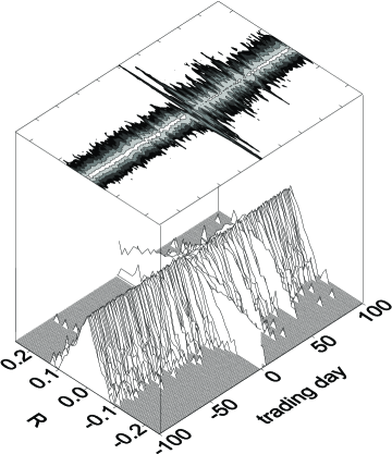
FIG. 1.: Contour and surface plot of the ensemble return distribution in a 200 trading days time interval centered at 19 October 1987 (corresponding to 0 in the abscissa). The probability density scale ($z$-axis) of the surface plot is logarithmic. The contour plot is obtained for equidistant intervals of the logarithmic probability density. The brightest area of the contour plot corresponds to the most probable value.

At the crisis, the ensemble distribution moves towards negative returns and then begins to oscillate between positive and negative returns. These oscillations are clearly evident for an interval of $70$ trading days after the 1987 crash. In that case, this is the time interval the market needed to come back to a ’typical’ state. This phenomenon is partly reflected into the oscillatory behavior of the Standard and Poor’s 500 index (S&P500) observed after the 1987 crash [6].

It is worth to investigate the changes of the ensemble return PDF not only by investigating the tails of the distribution but also its central part. In particular, it is important to understand whether in extreme days only the return mean value and the scale of the PDF are changed or if the shape of the PDF is modified also. To this end, we select the $9$ trading days of our database in which the S&P500 has negative extreme returns. We also consider the opposite case of the $9$ trading days in which the S&P500 has the greatest positive returns. These days are listed in Table I with the corresponding S&P500 return value. In Figure 2 and 3 we show the return distributions observed in the New York Stock Exchange in the days of extreme absolute returns. Specifically, Figure 2 shows the return distribution in crash days whereas Figure 3 shows the return distribution in rally days. Figure 2 shows that in crash days the PDF has a peak at a negative value of return. Moreover the distribution is asymmetric and the positive tail is steeper than the negative one. Therefore in crash days not only the scale but also the shape and symmetry properties of the distribution change.

FIG. 2.: Linear-log plot of the ensemble return distribution in days of S&P500 index extreme negative return occurring in the investigated time period (listed in the first part of Table I).

FIG. 3.: Linear-log plot of the ensemble return distribution in days of greatest S&P500 index positive return occurring in the investigated time period (listed in the second part of Table I).

A specular behavior is observed during the days of great gain of the market. Figure 3 shows that in these trading days the negative tail of the distribution is steeper than the positive one and the distribution has a peak at a positive return.

These findings can be quantified by noting that the distribution is negatively skewed in crash days, whereas the distribution is positively skewed in days of great gains. A quantitative estimate of the asymmetry of the PDF is difficult in finite statistical sets because the skewness parameter depends on the third moment of the distribution. Moments higher than the second are essentially affected by rare events rather than by the central part of the distribution. Due to the finite number of stocks in our statistical ensemble, a measure of the asymmetry of the distribution based on its skewness is not statistically robust. We overcome this problem by considering a different measure of the asymmetry of the distribution. Specifically, we extract the median and the mean of the distribution for all trading days. When a probability distribution is symmetric the median coincides with the mean. Therefore the difference between the mean and the median is a measure of the degree of asymmetry of the distribution. For positively (negatively) skewed distribution the median is smaller (greater) than the mean. The median depends weakly on the rare events of the random variable and therefore is much less affected than the skewness by the finiteness of the number of records of the ensemble. In order to estimate the median value we construct an histogram of the returns and we evaluate the median value as the value for which the area of the histogram below and above it are equal.

Figure 4 shows the difference between the mean and the median as a function of the mean for each trading day of the investigated period. In the Figure each circle refers to a different trading day. The circles cluster in an asymmetrical pattern which resembles a sigmoid shape. In days in which the mean is positive (negative) the difference between mean and median is positive (negative). In extreme days (for example those listed in Table I) the corresponding circles are characterized by great absolute value of the the mean and a great value of the difference between mean and median. Another result summarized in Figure 4 is that this effect is not exclusive of the days of extreme crash and rally but it is also evident for trading days of intermediate absolute average return. The change of the shape and of the symmetry properties during the days of large absolute returns suggests that in extreme days the behavior of the market cannot be statistically described in the same way of the ’normal’ periods. Moreover Figure 4 indicates that the difference from normal to extreme behavior increases gradually with the absolute value of the average return.

Among the extreme days one circle does not cluster around the sigmoid shape and shows a different behavior having a negative mean but a positive difference between mean and median. This circle (indicated by an arrow in Figure 4) corresponds to the 20 October 1987 day, which is the day after the black Monday. The ensemble return distribution for this day is shown in panel b of Figure 3. This day is quite anomalous because the S&P500 had a $5.24\%$ positive return, but the mean return of all the assets traded in NYSE was $-5.28\%$. In other words in this day companies performed returns which were strongly correlated with their capitalization. In summary, with just one exception, our results provide an empirical evidence that the ensemble statistical properties of a set of stocks traded simultaneously in a financial market change in a systematic way when the market moves far from the typical day characterized by a small average return.

We now compare the results of our empirical analysis with the results obtained by modeling the stock price dynamics with a simple model: the single-index model. The single-index model [10, 11] assumes that the returns of all assets are controlled by one factor, usually called the market.

FIG. 4.: Each circle is the difference between the mean and the median of the ensemble return distribution as a function of the mean for each trading day of the investigated time period. The arrow indicates the anomalous behavior of the day after October 1987 black Monday. In the inset we show the same quantity for the artificial data generated according to the single-index model. The scale of the inset is the same of the scale of the figure.

For any asset $i$, we have

$$R_{i}(t)=\alpha_{i}+\beta_{i}R_{M}(t)+\epsilon_{i}(t),$$ (2)

where $R_{i}(t)$ and $R_{M}(t)$ are the return of the asset $i$ and of the market at day $t$, respectively, $\alpha_{i}$ and $\beta_{i}$ are two real parameters and $\epsilon_{i}(t)$ is a zero mean noise term characterized by a variance equal to $\sigma^{2}_{\epsilon_{i}}$. The noise terms of different assets are uncorrelated, $<\epsilon_{i}(t)\epsilon_{j}(t)>=0$ for $i\neq j$. Moreover the covariance between $R_{M}(t)$ and $\epsilon_{i}(t)$ is set to zero for any $i$.

Each asset is correlated with the market and the presence of such a correlation induces a correlation between any pair of assets. It is customary to adopt a broad-based stock index for the market $R_{M}(t)$. Our choice for the market is the Standard and Poor’s 500 index. The best estimation of the model parameters $\alpha_{i}$, $\beta_{i}$ and $\sigma^{2}_{\epsilon_{i}}$ is usually done with the ordinary least squares method [11]. To compare our empirical results with the predictions of the single-index model we build up an artificial stock market following Eq. (2). This is done by first evaluating the model parameters for all the assets traded in the NYSE and then by generating a set of $n$ surrogate time series according to Eq. (2).

The ensemble return distribution computed in the artificial stock market is symmetrical in ’typical’ trading days. In crash and rally days, it is still approximately symmetrical around the mean value which can be positive (rallies) or negative (crashes). By contrast, as noted above, the return distribution in the real ensemble is asymmetric in extreme days. We can again quantify the asymmetry of the distribution by evaluating the difference between mean and median. The inset of Figure 4 shows the difference between the mean and the median as a function of the mean for the artificial data for each trading day of the investigated period. The differences between the real and artificial sets of circles are evident. The circles representing the synthetic data are distributed roughly symmetrically around the origin of the plane. Moreover the values of the difference between mean and median observed for the single-index model are not very large compared with the ones observed in the real set, confirming that the ensemble return distribution of the artificial data is approximately symmetrical in extreme days too. This difference suggests that the effective correlation among the assets can be described by the single-index model only as a first approximation. The degree of approximation of the single-index model progressively becomes worst for market days of increasing absolute average return and fails in properly describing the market behavior of extreme days.

The main object of this letter is the study of the return distribution of an ensemble of stocks in a trading day with extreme absolute average return. We show that the ensemble return distribution changes shape and symmetry properties in crash and rally days. We compare our empirical results with the expected behavior of the single-index model and we observe that this simple model fails in describing the market in extreme days. In particular the main discrepancy concerns the asymmetry of the ensemble return PDF of the model which is different from the one observed in empirical data in extreme days. Changes in the shape and symmetry of the PDF may be associated to changes of the correlation properties. It is commonly accepted that the return time series of different stocks synchronously traded are correlated and several researches has been performed in order to extract information from the correlation properties [3, 4, 5]. Our study suggests that the correlation properties between stocks may change during market days characterized by extreme absolute return. A precise characterization of the correlation properties and of their modification is of key importance for the modeling of market dynamics in normal and in extreme market days.

The authors thank INFM and MURST for financial support. This work is part of the FRA-INFM project ’Volatility in financial markets’. F. Lillo acknowledges an FSE-INFM fellowships. We wish to thank Giovanni Bonanno for help in numerical calculations.

TABLE I.: List of the $18$ days of the investigated period (from January 1987 to December 1998) in which the Standard and Poor’s 500 index has the greatest return in absolute value. The third column indicates the corresponding panel of the ensemble return distribution shown in Figures 2 and 3.

Date	Standard and Poor’s 500 return	Panel
19 10 1987	-0.2041	2a
26 10 1987	-0.0830	2b
27 10 1997	-0.0686	2c
31 08 1998	-0.0679	2d
08 01 1988	-0.0674	2e
13 10 1989	-0.0611	2f
16 10 1987	-0.0513	2g
14 04 1988	-0.0435	2h
30 11 1987	-0.0416	2i
21 10 1987	+0.0908	3a
20 10 1987	+0.0524	3b
28 10 1997	+0.0511	3c
08 09 1998	+0.0509	3d
29 10 1987	+0.0493	3e
15 10 1998	+0.0418	3f
01 09 1998	+0.0383	3g
17 01 1991	+0.0373	3h
04 01 1988	+0.0360	3i

REFERENCES

- [1] R. N. Mantegna and H. E. Stanley, An Introduction to Econophysics: Correlations and Complexity in Finance (Cambridge Univ. Press, 2000).
- [2] For a collection of papers see for example: R. N. Mantegna, ed., Proceedings of the International Workshop on Econophysics and Statistical Finance, Physica A 269, 1-187 (1999) Issue 1. J.-P. Bouchaud, ed., Proceedings of the International Conference on Applications of Physics in Financial Analysis”, Int. J. Theor. Appl. Finance, (in press).
- [3] R. N. Mantegna, Eur. Phys. J. B 11, (1999) 193 .
- [4] L. Laloux, P. Cizeau, J.-P. Bouchaud and M. Potters, Phys. Rev. Lett. 83, (1999) 1467.
- [5] V. Plerou, P. Gopikrishnan, B. Rosenow, L. A. N. Amaral and H. E. Stanley, Phys. Rev. Lett. 83, (1999) 1471.
- [6] D. Sornette, A. Johansen and J.-P. Bouchaud, J. Phys. I 6, (1996) 167.
- [7] D. Chowdhury and D. Stauffer, Eur. Phys. J. B 8, (1999) 477.
- [8] F. Lillo and R. N. Mantegna, Statistical Properties of Statistical Ensembles of Stock Returns, Int. J. Theor. Appl. Finance, (in press), cond-mat/9909302.
- [9] F. Lillo and R. N. Mantegna, Variety and Volatility in Financial Markets., (submitted).
- [10] E. J. Elton and M. J. Gruber Modern Portfolio Theory and Investment Analysis, (J. Wiley & Sons, New York, 1995).
- [11] J. Y. Campbell, A. W. Lo, A. C. MacKinlay The Econometrics of Financial Markets, (Princeton University Press, Princeton, 1997).