Nonlinear Effect of Transport Current on Response of Metals to Electromagnetic Radiation

Abstract

The nonlinear interaction of DC current flowing in a thin metal film with an external low-frequency AC electromagnetic field is studied theoretically. The nonlinearity is related to the influence of the magnetic field of the DC current and the magnetic field of the wave on the form of electron trajectories. This magnetodynamic mechanism of nonlinearity is the most typical for pure metals at low temperatures. We find that such interaction causes sharp kinks in the temporal dependence of the AC electric field of the wave on surface of the sample. The phenomenon of amplification of the electromagnetic signal on the metal surface is predicted. We also calculate the nonlinear surface impedance and show that it turns out to be imaginary-valued and its modulus decreases drastically with the increase of the wave amplitude.

I Introduction

As well-known metals possess quite peculiar nonlinear electrodynamic properties (see., for example, Refs. rev1 ; rev2 ). Indeed, nonlinearity in a response of plasma or semiconductors to an electromagnetic excitation is usually associated to significant deviation of the electron subsystem from equilibrium. To the contrary, nonequilibrium in metals as a rule is weak due to large concentration of charge carriers. Nevertheless, a nonlinear regime in these media is rather easy to observe. Such a situation is possible because of the fact that nonlinearity in metals does not necessarily related to the nonequilibrium of the electron subsystem. Nonequilibrium is caused by the existence of a weak electric field, while nonlinearity is originates from strong magnetic fields. The Lorentz force, determined by the magnetic field of an electromagnetic wave or magnetic field of the transport current, affects the dynamics of charge carriers. As a result, the conductivity of a sample placed in an AC electromagnetic field depends on the spatial distribution of magnetic field of the wave. Such a magnetodynamic mechanism of nonlinearity is inherent to pure metals at low temperatures, if the mean free path of conducting electrons is rather large.

Magnetodynamic nonlinearity causes a number of nontrivial phenomena in the electrodynamics of metals. As an example, one can mention generation of the current states Dolg ; CS in a sample placed in a DC external magnetic field. The sample acquires a DC magnetic moment if irradiated by an additional strong AC electromagnetic field. The magnitude of the magnetic moment depends in a hysteretic manner on an external DC magnetic field. Under current states conditions, a hysteresis-like interaction of radiowaves is observed int as well as the appearance of electromagnetic dissipative structures diss . This specific mechanism of nonlinearity in metals causes a decrease of collisionless damping of helicons helic1 . Therefore, the spiral waves with large amplitudes can propagate even in conditions when there is no their linear electromagnetic excitations helic2 . Magnetoplasmic shock waves shock and soliton-like excitations waves are also predicted for the regime of strong magnetodynamic nonlinearity.

In the present paper, we study a novel manifestation of magnetodynamic nonlinearity, namely, interaction of an external electromagnetic wave and a strong DC transport current in a thin metal film, which is also displayed in a quite unusual way. The sample of thickness $d$ is assumed to be much smaller than electron mean free path $l$,

$$d\ll l,$$ (1)

and electron scattering on a surface of the film is supposed to be diffuse. It is known Snapiro that in the static case (when external AC signal is absent), the magnetic field of a current can essentially affect the conductivity of a thin metal specimen and, thus, its current-voltage characteristics (CVC). In this situation the value $I$ of the current is rather small so that the typical radius of curvature $R(I)$ of electron trajectories in magnetic field is much greater than the film thickness,

$$d\ll R(I),\qquad\qquad R(I)=cp_{F}/eH(I)\propto I^{-1}.$$ (2)

Here $-e$ and $p_{F}$ represent electron charge and Fermi momentum, respectively. In Ref. Snapiro , it was shown that nonlinear peculiarities of CVC are connected to the antisymmetrical spatial distribution of the magnetic field of the DC current inside the sample. The magnetic field equals to zero at the middle of the film and takes the values $H$ to $-H$ at the opposite boundaries of the sample, where

$$H=2\pi I/cD.$$ (3)

In this formula, $c$ denotes the speed of light in vacuum and $D$ is the sample width. Spatially alternating field of the DC current entraps a part of electrons in a potential well. Trajectories of such particles are flat curves winding around the plane of alternation of the magnetic field. The relative part of the trapped electrons in the order of magnitude is equal to the typical angle $(d/R)^{1/2}\ll 1$ of their crossing of that plane. Taking into account that trapped carriers do not collide with the film boundaries and interact with the electric field along their whole free path $l$, one can write the following estimating formula for their conductivity $\sigma_{tr}$:

$$\sigma_{tr}\sim\sigma_{0}(d/R(I))^{1/2}\propto I^{1/2}.$$ (4)

Here $\sigma_{0}$ represents the conductivity of the bulk sample. At the same time, there exist flying electrons which do collide with the boundaries of the specimen and, according to Ref. Fuks , have the conductivity of the order of $\sigma_{0}(d/l)$. Apparently in the range of rather strong currents, when the inequality

$$(dR(I))^{1/2}\ll l,$$ (5)

holds, the conductivity of the film is determined by the group of the trapped carriers. As a result, we observe the deviation from the Ohm’s law: the voltage $U$ is proportional to the square root of current,

$$U\propto I^{1/2}.$$ (6)

For the film with thickness $d=10^{-3}$ cm, the electron mean free path $l=10^{-1}$ cm, and Fermi momentum $p_{F}=10^{-19}$ g$\cdot$ cm/s the nonlinearity becomes noticeable ($(dR)^{1/2}\sim~{}l$) at values of the magnetic field $H(I)$ about $1$ Oe. The theory developed in Ref. Snapiro is in a good qualitative agreement with experimental data (see, for example, Ref. Fish1 ).

In an external magnetic field $\bf h$, collinear to the magnetic field of the current, the plane of the sign alternation for the magnetic field shifts to one of the two boundaries of the film (see Fig. 1). That in turn leads to appreciable diminution of the number of the trapped particles and, therefore, their conductivity. In particular, such a situation would take place under symmetrical irradiation of the film by the low-frequency electromagnetic wave of large amplitude. The frequency is supposed to be so small that the AC magnetic field ${\bf h}(t)$ of the wave is virtually uniform across the metal (i.e. the wave penetration depth $\delta$ is much greater than the sample thickness $d$). Then the conductivity of metal essentially depends on time and, therefore, strong nonlinear effects in the sample response to the AC electromagnetic excitation should appear. Being of interest from the both theoretical and experimental points of view this problem has not been investigated yet.

In the present paper we study theoretically the temporal dependence of electric field at the surface of the film, which carries a strong DC current of the fixed value $I$ satisfying inequalities (2) and (5). It is shown that with an increase of the amplitude $h_{m}$ of the AC magnetic field this dependence becomes anharmonic, turning into a series of sharp nonanalytic peaks. The case of sufficiently high amplitudes $h_{m}>H$, when the total magnetic field in the sample is spatially alternating during some part of the wave period and has constant sign during the other part, is of particular interest. In such a situation, the electric field is also characterized by kinks in its temporal dependence due to the periodical appearance and disappearance of the group of trapped carriers. The effect of amplification of the electric signal on the film surface is predicted as well. It turns out that, because of the presence of the strong DC transport current in the sample, the absolute value of the AC electric field of the wave is $l/(dR)^{1/2}\gg 1$ times as many as the corresponding magnitude in the absence of the DC current.

We also calculate the nonlinear surface impedance of the film, which turns out to be pure imaginary value in the main approximation in the parameter $d/\delta\ll 1$, and show that its modulus monotonically diminishes with the growth of the AC amplitude decreasing in $l/(dR)^{1/2}\gg 1$ times. Simultaneously the conductivity of the trapped particles falls down and, consequently, $\delta$ increases.

II Problem statement and geometry

Consider a metal film of the thickness $d$ with a DC current $I$ flowing along. The sample is irradiated from both sides by a monochromatic electromagnetic wave with a magnetic component collinear to the magnetic field of the current. The $x$-axis is oriented perpendicularly to the film boundaries. The plane $x=0$ corresponds to the middle of the sample (see Fig. 1).

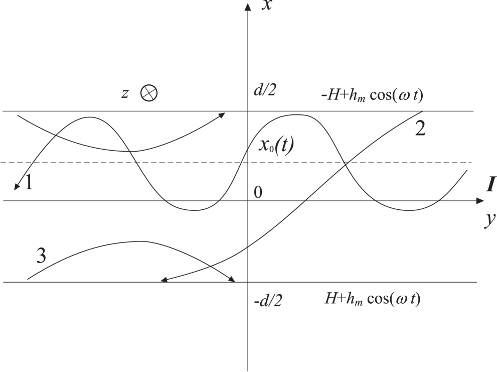
Figure 1: Geometry of problem. Schematic representation of the trajectories of trapped (1), flying (2), and surface (3) electrons.

The $y$-axis is directed along the current, and the $z$-axis is parallel to the vector ${\bf{\cal H}}(x,t)$ of the total magnetic field which is a sum of the DC magnetic field of the current ${\bf H}(x,t)$ and the AC magnetic field of the wave ${\bf h}(x,t)$,

$${\bf{\cal H}}(x,t)=\{0,0,H(x,t)+h(x,t)\}.$$ (7)

The film length $L$ (the dimension along the $y$-axis) and its width $D$ ($z$-axis dimension) are much greater than the sample thickness $d$. We assume diffuse scattering of the electrons on the film boundaries. Maxwell’s equations in the assumed geometry can be written as

$$-\frac{\partial{\cal H}(x,t)}{\partial x}=\frac{4\pi}{c}j(x,t),\qquad\frac{\partial E(x,t)}{\partial x}=-\frac{1}{c}\frac{\partial{\cal H}(x,t)}{\partial t},$$ (8)

where $j(x,t)$ and $E(x,t)$ represent the $y$ components of the current density and the electric field. Boundary conditions for Eqs. (8) are

$${\cal H}(\pm d/2,t)=h_{m}\cos\omega t\mp H.$$ (9)

Let $H$ be the absolute value of the magnetic field on the surface of the metal film and $h_{m}$ denote a wave amplitude. According to Eq. (3), the field $H$ is determined by the DC current $I$. No special relation between magnitudes $H$ and $h_{m}$ is assumed.

We consider a quasistatic situation when the wave frequency $\omega$ is much less than the relaxation frequency $\nu$ of the charge carriers,

$$\omega\ll\nu.$$ (10)

Here we suppose that the AC magnetic field inside the sample is quasiuniform and virtually does not differ from its value on the sample surface, $h(x,t)\simeq h_{m}\cos\omega t$. In other words, the typical spatial scale $\delta(\omega)$ of variation of the AC magnetic field is much greater than the film thickness $d$. Furthermore we assume that the curvature radius $R(x,t)$ of electron trajectories in the total magnetic field ${\cal H}(x,t)$ is also much greater than $d$,

$$d\ll\delta(\omega),\qquad d\ll R(x,t),\qquad R(x,t)=cp_{F}/e|{\cal H}(x,t)|.$$ (11)

III Electron dynamics, current density, and CVC of film

Let us consider electron dynamics in the nonuniform AC magnetic field ${\cal H}(x,t)$. We shall assume the following gauge of the vector potential:

$${\bf A}(x,t)=\{0,A(x,t),0\},\qquad A(x,t)=\int^{x}dx^{\prime}{\cal H}(x^{\prime},t).$$ (12)

It is suitable to choose the lower limit of integration in Eq. (12) depending on whether or not there exists the plane $x=x_{0}(t)$ of the sign alternation of the magnetic field ${\cal H}(x,t)$ at the present moment. This plane exists during the time intervals when $h_{m}|\cos\omega t|<H$ because the values $h_{m}\cos\omega t-H$ and $h_{m}\cos\omega t+H$ of the total magnetic field at the film boundaries have opposite signs (see Eq. (9)). In this case, one should take $x_{0}(t)$ as the lower limit in integral (12). Then the vector potential $A(x,t)$ is negative. It reaches its maximum value (which equals to zero) at the point $x=x_{0}(t)$. Within other time intervals, when the inequality $h_{m}|\cos\omega t|>H$ holds, the magnetic field ${\cal H}(x,t)$ inside the sample is of a constant sign. In such a situation, one should choose ${\rm sign}(\cos\omega t)d/2$ (${\rm sign}(x)$ is the sign function) as a lower limit of the integration. In this case, vector potential, also being negative, vanishes at one of the boundaries of the film.

The integrals of motion of electron in the field ${\cal H}(x,t)$ are the total energy (it equals to the Fermi energy) and the canonical momenta $p_{z}=mv_{z}$ and $p_{y}=mv_{y}-eA(x,t)/c$ (m is the electron mass). The electron trajectory in a perpendicular to the direction of the magnetic field plane is determined by the velocities $v_{x}(x,t)$ and $v_{y}(x,t)$. In the case of Fermi-sphere with radius $p_{F}=mv$, we obtain

$$|v_{x}(x,t)|=(v_{\bot}^{2}-v_{y}^{2})^{1/2},\ \ v_{\bot}=(v^{2}-v_{z}^{2})^{1/2},\ \ v_{y}(x,t)=(p_{y}+eA(x,t)/c)/m.$$ (13)

Classically allowable regions of the electron motion along the $x$ axis are determined by the inequalities,

$$-p_{y}-mv_{\bot}\leq eA(x,t)/c\leq-p_{y}+mv_{\bot}.$$ (14)

These inequalities provide the positivity of the radicand in Eq. (13) for $|v_{x}(x,t)|$.

The regions of the electron motion in the phase plane $(x,p_{y})$ are described schematically in Fig. 2 for two cases: when there exists the plane $x=x_{0}(t)$ of the sign alternation of the magnetic field ${\cal H}(x,t)$ (Fig. 2, a) and when such plane is absent (Fig. 2, b).

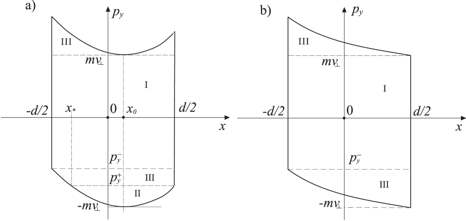
Figure 2: Phase space $(p_{y},x)$. Regions of existence of flying (I), trapped (II), and surface (III) particles in spatially sign alternating (a) and of constant sign (b) total magnetic field.

For definiteness we have chosen the moment of time when the magnetic field of the wave is positive ($\cos\omega t>~{}0$). The upper border on the phase plane is described by the curve $p_{y}=mv_{\bot}-eA(x,t)/c$ and the lower one is given by $p_{y}=-mv_{\bot}-eA(x,t)/c$. The electrons are naturally divided in three groups depending on the sign and value of the integral of motion $p_{y}$. Below, we give inequalities determining the regions of their existence at an arbitrary moment of time.

1. Flying electrons:

   $$p_{y}^{-}\equiv-mv_{\bot}-eA[-{\rm sign}(\cos\omega t)d/2,t]/c\leq p_{y}\leq mv_{\bot},\qquad|x|\leq d/2.$$ (15)

   These particles collide with the both boundaries of the film. Their trajectories do not twist significantly because of $d\ll R(x,t)$. Flying electrons exist at every moment of time irrespective of the presence of the plane $x=x_{0}(t)$ (i.e irrespective of the relation between $h_{m}\cos\omega t$ and $H$).

2. Trapped electrons: They appear during the periods of time when $h_{m}|\cos\omega t|<H$ and the total magnetic field ${\cal H}(x,t)$ within the sample passes trough zero. Their states are bounded by the region (see. Fig. 2,a),

   $$-mv_{\bot}\leq p_{y}\leq p_{y}^{+}\equiv-mv_{\bot}-eA[{\rm sign}(\cos\omega t)d/2,t]/c,$$

   $$x_{*}(t){\rm sign}(\cos\omega t)<x{\rm sign}(\cos\omega t)<d/2.$$ (16)

   Here $x_{*}(t)$ represents the breakpoint of the trapped electron most distant from the film boundary. One can find it from the equation,

   $$A(x_{*},t)=A[{\rm sign}(\cos\omega t)d/2,t].$$ (17)

   According to Eq. (16), this electron group occupies the region $x_{*}(t)<x<~{}d/2$ when $\cos\omega t>0$ and the region $-d/2<x<x_{*}(t)$ if $\cos\omega t<0$. The trajectories of trapped particles are almost flat oscillating curves due to periodical motion of the particles along $x$-direction and the uniform motion along the $y$-and $z$-axes. The temporal period of oscillations with respect to the plane $x=x_{0}$ equals to $2T$, where

   $$T=\int^{x_{2}(t)}_{x_{1}(t)}\frac{dx}{|v_{x}(x,t)|}.$$ (18)

   The breakpoints $x_{1}(t)$ and $x_{2}(t)$ ($x_{1}(t)<x_{0}(t)<x_{2}(t)$) are the roots of the equation,

   $$eA(x_{1,2},t)/c=-mv_{\bot}-p_{y}.$$ (19)

3. Surface electrons:

   These particles collide only with one of the boundaries of the film. In our case of diffuse scattering of the electrons on the surface, their influence on the nonlinear conductivity of metal is negligible Snapiro . Thus, we do not take them into account thereafter.

The current density of the flying and trapped particles can be deduced by means of solving the Boltzmann kinetic equation. One should linearize the kinetic equation with respect to the electric field $E(x,t)$, which can be represented as a sum,

$$E(x,t) = E_{0}+{\cal E}(x,t),$$

$${\cal E}(x,t) = -\frac{1}{c}\left(\frac{\partial A(x,t)}{\partial t}-\frac{\partial\bar{A}(t)}{\partial t}\right).$$ (20)

Here the first term, $E_{0}$, is a potential (uniform) component and ${\cal E}(x,t)$ is a rotational (nonuniform) field of the wave. Spatial averaging of the latter over the $x$-axis direction gives zero. The value $\bar{A}(t)$ represents a spatially averaged magnitude of the vector potential,

$$\bar{A}(t)=\frac{1}{d}\int^{d/2}_{-d/2}A(x^{\prime},t)dx^{\prime}.$$ (21)

The magnetodynamic nonlinearity is accounted for in the kinetic equation by means of terms which contain the total magnetic field ${\cal H}(x,t)=H(x,t)+h(x,t)$ entering the Lorentz force. We calculate the current density in the main approximation with respect to the small parameter $d/\delta(\omega)$ (see Eq. (11)). In this approximation, as it was mentioned above, the AC magnetic field $h(x,t)$ becomes spatially uniform and is equal to its boundary value, $h(x,t)=h_{m}\cos\omega t$. The electric field is also independent of the $x$-coordinate and coincides with the value $E_{0}(t)$. For the case of uniform electric and external magnetic fields, the current density was obtained in Ref. Snapiro . If the conditions (2) and (5) hold the following asymptotics for the current density of the flying and trapped electrons are valid:

$$j_{fl}(t)=\sigma_{fl}(t)E_{0}(t),$$

$$\sigma_{fl}(t)=\frac{3}{8}\sigma_{0}\frac{d}{l}\ln\frac{R_{+}(t)}{d},\quad R_{\pm}(t)=cp_{F}/e|h_{m}|\cos\omega t|\pm H|,$$ (22)

$$j_{tr}(x,t)=\sigma_{tr}(x,t)E_{0}(t),$$

$$\sigma_{tr}(x,t)=\frac{36\pi^{1/2}}{5\Gamma^{2}(1/4)}\sigma_{0}\Big{\{}\frac{e}{cp_{F}}\left[A(x,t)-A({\rm sign}(\cos\omega t)d/2,t)\right]\Big{\}}^{1/2},$$ (23)

$$x_{*}(t){\rm sign}(\cos\omega t)<x{\rm sign}(\cos\omega t)<d/2.$$

In the limit $\omega\to 0$, Eqs. (22) and (23) transform into the corresponding formulae of Ref. Snapiro .

Let us substitute the current density in the first of Maxwell’s equations (8) for its asymptotic expressions (22) and (23) and introduce a dimensionless coordinate and vector potential,

$$\xi=2x{\rm sign}(\cos\omega t)/d,\qquad a(\xi,t)=A(x,t)/A({\rm sign}(\cos\omega t)d/2,t).$$ (24)

The equation for the quantity $a(\xi,t)$ has the form,

$$\frac{\partial^{2}a(\xi,t)}{\partial\xi^{2}}=u\cases{r[1-a(\xi,t)]^{1/2}+1,&$\xi_{*}(t)\leq\xi\leq 1$,\cr&\cr 1,&$-1\leq\xi\leq\xi_{*}(t),$\cr}$$ (25)

$$\xi_{*}(t)=2x_{*}(t){\rm sign}(\cos\omega t)/d.$$ (26)

The dimensionless coordinate $\xi_{*}(t)$ confines the region of existence of the trapped particles and, according to Eqs. (17) and (24), satisfies the equation, $a(\xi_{*},t)=1$. The parameter $r$ represents the ratio of the maximum magnitude of the conductivity of the trapped electrons to the conductivity of the flying particles,

$$r=\frac{\sigma_{tr}(x_{0})}{\sigma_{fl}}=\frac{96\pi^{1/2}}{5\Gamma^{2}(1/4)}\frac{l}{d}\left[\frac{e}{cp_{F}}|A({\rm sign}(\cos\omega t)d/2,t)|\right]^{1/2}\ln^{-1}(R_{+}/d).$$ (27)

The dimensionless quantity, $u$, is related to the voltage $U=E_{0}L$ on the sample,

$$u=\frac{U}{cL|A({\rm sign}(\cos\omega t)d/2,t)|/\pi\sigma_{fl}d^{2}}.$$ (28)

Equation (25) should be solved together with the boundary conditions,

$$\frac{\partial a(1,t)}{\partial\xi}=\frac{d}{2}\frac{h_{m}|\cos\omega t|-H}{A({\rm sign}(\cos\omega t)d/2,t)},$$

$$\frac{\partial a(-1,t)}{\partial\xi}=\frac{d}{2}\frac{h_{m}|\cos\omega t|+H}{A({\rm sign}(\cos\omega t)d/2,t)},\quad a(1,t)=1.$$ (29)

The first two of these expressions are dimensionless boundary conditions (9), and the third one is a consequence of normalization (24) of the vector potential.

Within the interval $\xi_{*}(t)\leq\xi\leq 1$, the solution of Eq. (25) is symmetrical with respect to the point $\xi_{0}(t)=(1+\xi_{*}(t))/2$, where the dimensionless vector potential reaches its minimum value (which equals to zero, $a(\xi_{0},t)=\partial a(\xi_{0},t)/\partial\xi=0$). This solution is described by the formula,

$$|\xi-\xi_{0}(t)|=(3/4ru)^{1/2}\int_{0}^{a(\xi,t)}d\zeta[1-(1-\zeta)^{3/2}+3\zeta/2r]^{-1/2}.$$ (30)

One can not obtain the field distribution and the current density within the region of existence of the trapped electrons in an explicit form. However, by means of Eq. (30), it is possible to calculate the average magnitude of the conductivity of the trapped carriers (23) within the interval (16),

$$\frac{{\bar{\sigma}_{tr}}}{\sigma_{fl}} = r\int_{0}^{1}d\zeta(1-\zeta)^{1/2}[1-(1-\zeta)^{3/2}+3\zeta/2r]^{-1/2}$$ (31)

$$\times \left(\int_{0}^{1}d\zeta[1-(1-\zeta)^{3/2}+3\zeta/2r]^{-1/2}\right)^{-1}.$$

The bar above $\sigma_{tr}$ denotes spatial averaging. In the remaining region of the sample ($-1\leq\xi\leq\xi_{*}(t)$), there exist only flying electrons, and the solution of Eq. (25) is given by the following formula:

$$a(\xi,t)=1-(2u)^{1/2}(1+2r/3)^{1/2}(\xi-\xi_{*}(t))+u(\xi-\xi_{*}(t))^{2}/2.$$ (32)

Expressions (30) and (32) and their derivatives are sewn together at the point $\xi=\xi_{*}(t)$. The solution given by Eqs. (30) and (32) contains three parameters, $\xi_{0}$, $u$ and $r$, which should be found from boundary conditions (29). It is essential that the value $A({\rm sign}(\cos\omega t)d/2,t)$ of the vector potential appearing in Eq. (29) is not an independent parameter due to its relation to $r$ via formula (27).

Adding term by term the first two boundary conditions in Eq. (29) and using Eqs. (30) and (32), and (28), we find the following expression for the drift of the plane $x=x_{0}$:

$$\xi_{0}=2x_{0}{\rm sign}(\cos\omega t)/d=\frac{Lh_{m}|\cos\omega t|}{2\pi U\sigma_{fl}d},\qquad h_{m}|\cos\omega t|\leq H.$$ (33)

In order to determine the value of $u$ (i.e. the voltage $U$), let us integrate the left and right-hand sides of Eq. (25) from -1 to 1 taking into account the boundary conditions for the derivative $\partial a(\xi,t)/\partial\xi$ in (29). The integral of the function $[1-a(\xi,t)]^{1/2}$ appearing in the right-hand side can be reduced to the product $2(1-\xi_{0}){\bar{\sigma}_{tr}}/r\sigma_{fl}$ with the use of the condition $a(1,t)=1$. Taking this into consideration as well as formulae (28) and (33) for the quantities $u$ and $\xi_{0}$, we have after some simple transformations,

$$U=\frac{cL}{2\pi d\sigma_{fl}(t)}\frac{H(I)+({\bar{\sigma}_{tr}}/\sigma_{fl})h_{m}|\cos\omega t|}{1+{\bar{\sigma}_{tr}}/\sigma_{fl}},\qquad h_{m}|\cos\omega t|\leq H.$$ (34)

According to Eq. (31), the ratio of conductivities, ${\bar{\sigma}_{tr}}/\sigma_{fl}$, depends on the parameter $r$. Using expression (28) for $u$, relation (27) between $A({\rm sign}(\cos\omega t)d/2,t)$ and $r$, and solution (30), we obtain from the first boundary condition in Eq. (29) the algebraic equation for $r$,

$$r^{2}(1+2r/3)=\left(\frac{H-h_{m}|\cos\omega t|}{{\tilde{H}}}\right)^{2}\frac{{\tilde{U}}}{U\ln^{3}(R_{+}/d)},\qquad h_{m}|\cos\omega t|\leq H.$$ (35)

Here we have introduced the following notations:

$${\tilde{H}}=\frac{25\Gamma^{4}(5/4)}{9\pi}\frac{cp_{F}d}{el^{2}},\qquad{\tilde{U}}=\frac{4clL{\tilde{H}}}{3\pi\sigma_{0}d^{2}}.$$ (36)

The parameters ${\tilde{H}}$ and ${\tilde{U}}$ represent those magnitudes of the magnetic field and voltage for which the characteristic length $(Rd)^{1/2}$ of the arch of electron’s trajectory is of the order of the mean free path $l$.

Expressions (31), (34), and (35) define, in an implicit form, dependence of the voltage $U$ on the current $I$ for the case $h_{m}|\cos\omega t|\leq H$. At these conditions there exists the plane of the alternation of sign of the total magnetic field within the sample. If the opposite inequality, $h_{m}|\cos\omega t|\geq H$, is valid, the trapped electrons are absent ($r=0$, $\xi_{*}=1$, $\sigma_{tr}=0$) and CVC is described by the formula,

$$U=\frac{cLH(I)}{2\pi d\sigma_{fl}(t)},\qquad h_{m}|\cos\omega t|\geq H.$$ (37)

As seeing from formula (34), the voltage on the sample displays nonanalytical behavior vs. time: the dependence $U(t)$ has kinks at the moments when the AC magnetic field $h_{m}\cos\omega t$ vanishes. This is an essentially nonlinear effect caused by the contribution of a large group of trapped electrons into the electric current.

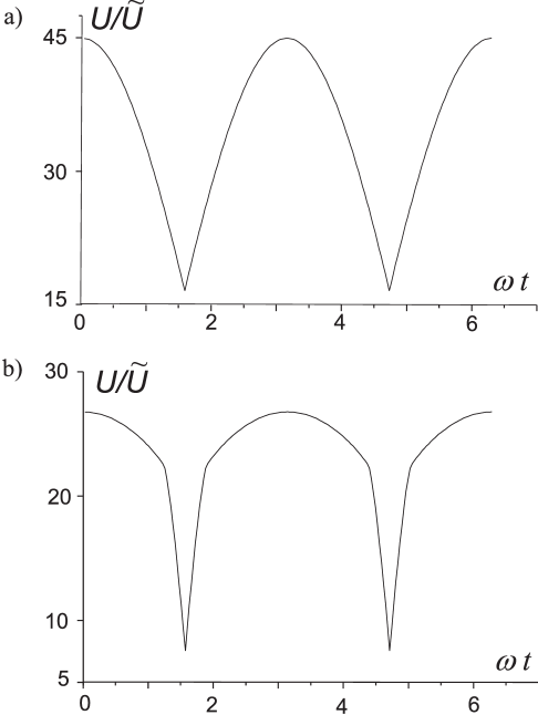
Figure 3: Time dependence of the voltage $U$ at relatively small (a, $h_{m}<H$) and large (b, $h_{m}>H$) AC amplitudes.

The temporal dependence of voltage (34) for the case when the wave amplitude is not too large ($h_{m}<H$) and there exist the trapped carriers during the whole period $2\pi/\omega$ is shown in Fig. 3, a. Fig. 3. b represents the dependence $U(t)$ for the opposite case $h_{m}>H$, in which during some part of the wave period (at $h_{m}|\cos\omega t|\geq H$) the conductivity is caused by the flying particles only.

IV Nonanalytical temporal dependence of electric field

Knowing the vector potential $A(x,t)$, one can calculate the rotational electric field ${\cal E}(x,t)$ as a correction to $E_{0}(t)$, (see Ref. (III)). We are interested in the difference $\Delta{\cal E}(t)={\cal E}(d/2,t)-{\cal E}(-d/2,t)$. This value is proportional to the rate of alteration of the magnetic flux trough the cross-sectional plane, which is perpendicular to the direction of the vector of the total field ${\bf{\cal H}}(x,t)$, and thus can be measured in experiment.

From Eqs. (30) and (32), it follows that the difference $a(1,t)-a(-1,t)$ is connected to the derivatives $\partial a(1,t)/\partial\xi$ and $\partial a(-1,t)/\partial\xi$ by the relations,

$$a(1,t)-a(-1,t)=-\xi_{0}(t)\left[\frac{\partial a(1,t)}{\partial\xi}-\frac{\partial a(-1,t)}{\partial\xi}\right],\qquad h_{m}|\cos\omega t|\leq H,$$ (38)

$$a(1,t)-a(-1,t)=\frac{\partial a(1,t)}{\partial\xi}+\frac{\partial a(-1,t)}{\partial\xi},\qquad h_{m}|\cos\omega t|\geq H.$$ (39)

Let us now turn to the dimensional variables in Eqs. (38) and (39) using boundary conditions (29) and relation (27) between the values of $A({\rm sign}(\cos\omega t)d/2,t)$ and $r$. After that one can obtain the following expression for the magnitudes of the vector potential at the film boundaries:

$$A({\rm sign}(\cos\omega t)d/2,t)=-{\tilde{H}}d\ln^{2}(R_{+}/d)r^{2}/4,$$

$$A(-{\rm sign}(\cos\omega t)d/2,t)=-{\tilde{H}}d\ln^{2}(R_{+}/d)r^{2}/4-2H|x_{0}(t)|$$ (40)

at

$$h_{m}|\cos\omega t|\leq H$$

and

$$A({\rm sign}(\cos\omega t)d/2,t)=0,\quad A(-{\rm sign}(\cos\omega t)d/2,t)=-dh_{m}|\cos\omega t|$$ (41)

at

$$h_{m}|\cos\omega t|\geq H.$$

Formulae (40) and (41) are sewn at the time moment when $h_{m}|\cos\omega t|=H$. The parameter $r$ in Eq. (27) vanishes, and the plane $x=x_{0}(t)$ coincides with one of the boundaries of the sample, $|x_{0}(t)|=d/2$. From relations (40) and (III), by means of formula (33) for $\xi_{0}(t)$, we derive the expression for the difference $\Delta{\cal E}(t)$ of magnitudes of the electric field at the film boundaries,

$$\Delta{\cal E}(t)=-\frac{2H}{c}\frac{\partial x_{0}(t)}{\partial t}=-\frac{H(I)Lh_{m}}{2\pi}\frac{\partial}{\partial t}\left[\frac{\cos\omega t}{\sigma_{fl}(t)U(t)}\right],\qquad h_{m}|\cos\omega t|\leq H.$$ (42)

If the inequality $h_{m}\leq H$ holds, the previous relation is valid during the whole period of the wave. However, in the case $h_{m}>H$, there exists a time interval when the plane $x=x_{0}(t)$ of alternation of the sign of the total magnetic field is absent. If such a situation takes place one should use formula (41) in order to obtain the dependence $\Delta{\cal E}(t)$. Finally we come to the result below,

$$\Delta{\cal E}(t)=\Delta{\cal E}_{L}\sin\omega t,\qquad\Delta{\cal E}_{L}=dh_{m}\omega/c,\qquad h_{m}|\cos\omega t|\geq H.$$ (43)

From this, it follows that the difference $\Delta{\cal E}(t)$ is a harmonic function of time, i.e. the response of the film on the external electromagnetic excitation turns out to be linear if there are no trapped electrons. It is obvious that formula (43) also describes the dependence $\Delta{\cal E}(t)$ at small magnitudes of the current $I$ ($H\ll{\tilde{H}}$), when the contribution of trapped particles to the conductivity is negligible during the whole period of the wave. Then the value $\Delta{\cal E}_{L}$ represents the amplitude of a linear response.

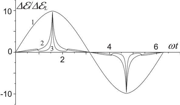
Figure 4: The dependence $\Delta{\cal E}(t)$ for $H=300{\tilde{H}}$ and various amplitudes of the AC signal: $h_{m}=1{\tilde{H}}$ (1), $h_{m}=200{\tilde{H}}$ (2), $h_{m}=500{\tilde{H}}$ (3).The ratio of the mean free path $l$ to the film thickness $d$ equals to 30.

The dependence $\Delta{\cal E}(t)$ is shown in Fig. 4 for a wide range of the AC amplitudes $h_{m}$ and for the large magnitudes of the DC magnetic field $H$ of the current $I$, when the inequality $H\gg{\tilde{H}}$ (or inequality (5)) is valid. It is obvious that the ratio of the amplitude $\Delta{\cal E}_{m}$ to its linear value $\Delta{\cal E}_{L}$ does not depend on $h_{m}$. From relations (42), (34), and (35) at $\cos\omega t=0$, we find the expression for $\Delta{\cal E}_{m}$,

$$\frac{\Delta{\cal E}_{m}}{\Delta{\cal E}_{L}}=0.83\left(\frac{H}{{\tilde{H}}}\right)^{1/2}\frac{1}{\ln(R/d)},\qquad\left(\frac{H}{{\tilde{H}}}\right)^{1/2}\sim\frac{\sigma_{tr}}{\sigma_{fl}}\Bigg{|}_{\cos\omega t=0}\sim\frac{l}{(Rd)^{1/2}}\gg 1.$$ (44)

The ratio $\Delta{\cal E}_{m}/\Delta{\cal E}_{L}$ is determined by the magnitude of the DC magnetic field $H$ and can be much greater than unity. In other words, there exists an effect of amplification of the electric signal at the film surface. For small AC amplitudes (curve $1$, $h_{m}=H/300$) the signal turns out to be quasi-harmonic. However, with the increase of $h_{m}$ the dependence $\Delta{\cal E}(t)$ shows kinks. Curve $2$ has kinks at the points of extremum, i.e at the time moments when the AC magnetic field $h_{m}\cos\omega t$ vanishes. These singularities are related to the nonanalytical behavior of CVC of the film (see. Eq. (34) and Fig. 3). Curve $3$ corresponds to the case $h_{m}=5H/3$, in which the trapped electrons are absent during a part of the wave period. In such a situation, the dependence $\Delta{\cal E}(t)$ contains additional kinks arising at the moments of appearance and disappearance of the plane $x=x_{0}(t)$ of the sign alternation of the total magnetic field. They are located symmetrically with respect to the points of extremum as shown in curve $3$. By means of formulae (42), (43),(34), and (35), we find the right and left derivatives of the function $\Delta{\cal E}(t)$ at the point $t_{0}=(1/\omega)\arccos(H/h_{m})$ of the first kink,

$$\frac{\partial}{\partial t}\frac{\Delta{\cal E}(t)}{\Delta{\cal E}_{L}}\Bigg{|}_{t=t_{0}-0}=\frac{\omega H}{h_{m}},$$ (45)

$$\frac{\partial}{\partial t}\frac{\Delta{\cal E}(t)}{\Delta{\cal E}_{L}}\Bigg{|}_{t=t_{0}+0}=\frac{\omega H}{h_{m}}\left[1-\frac{\pi}{2\ln(R_{+}/d)}\left(\frac{H}{\tilde{H}}\right)^{1/2}\left(\frac{h_{m}^{2}}{H^{2}}-1\right)\right].$$ (46)

According to Eq. (46), the right derivative is negative and has large absolute value even at $[(h_{m}/H)^{2}-1]\geq 1$.

V Surface impedance of film

Let us analyze the dependence of the surface impedance at the film boundary $x=d/2$ on the AC amplitude $h_{m}$ under conditions of interaction of the transport current and the electromagnetic wave. The impedance is proportional to the ratio of the first Fourier harmonics of the electric ${\cal E}_{\omega}$ and magnetic $h_{\omega}$ fields at the surface of the sample,

$$Z=\frac{4\pi}{c}\frac{{\cal E}_{\omega}}{h_{\omega}} =\frac{8\pi}{c}\frac{{\cal E}_{\omega}}{h_{m}},\quad{\cal E}_{\omega}=-\frac{\omega}{2\pi c}\int^{2\pi/\omega}_{0}\left(\frac{\partial A(d/2,t)}{\partial t}-\frac{\partial\bar{A}}{\partial t}\right)e^{{\rm i}\omega t}dt$$ (47)

$$=\frac{{\rm i}\omega^{2}}{2\pi c}\int^{2\pi/\omega}_{0}\left(A(d/2,t)-\bar{A}(t)\right)e^{{\rm i}\omega t}dt.$$

Taking into account Eqs. (33) and (40), we deduce the boundary value of the vector potential for the periods of time given by the inequality $h_{m}|\cos\omega t|\leq H$,

$$A(d/2,t)=\left\{\begin{array}[]{ll}-{\tilde{H}}d\ln^{2}(R_{+}/d)r^{2}/4,\,at\cos\omega t>0,&\\ -{\tilde{H}}\ln^{2}(R_{+}/d)r^{2}/4+cHLh_{m}\cos\omega t/2\pi U(t)\sigma_{fl}(t),\,at\cos\omega t<0.&\end{array}\right.$$ (48)

In the case $h_{m}|\cos\omega t|\geq H$, the following expression is valid (see. Eq. (41)):

$$A(d/2,t)=\cases{0,&$\quad at\cos\omega t>0$,\cr dh_{m}\cos\omega t,&$\quad at\cos\omega t<0$.}$$ (49)

Let us calculate the mean value of the vector potential $\bar{A}(t)$ for $h_{m}|\cos\omega t|\leq H$, when there exists the plane of alternation of sign of the field. According to Eqs. (30) and (32), we have

$$\frac{\bar{A}(t)}{A({\rm sign}(\cos\omega t)d/2,t)}=\frac{1}{2}\int^{1}_{-1}a(\xi,t)d\xi=\xi_{0}(t)+(2u(t))^{1/2}(1+r(t)/3)^{1/2}\xi^{2}_{0}(t)$$

$$+(2/3)u(t)\xi^{3}_{0}+\left(\frac{3}{4r(t)u(t)}\right)^{1/2}\int^{1}_{0}\frac{\zeta d\zeta}{\sqrt{1-(1-\zeta)^{3/2}+3\zeta/2r(t)}}.$$ (50)

In the case $h_{m}|\cos\omega t|\geq H$, one should use solution (32) with $r=0$, $\xi_{*}=1$ in order to find $\bar{A}(t)$. Proceeding to dimensional variables and using Eqs. (28) and (37), one can easily obtain

$$\bar{A}(t)=-\frac{dh_{m}|\cos\omega t|}{2}-\frac{1}{6}Hd.$$ (51)

We draw reader’s attention to the fact that the mean value of the vector potential depends on time only via the term $|\cos\omega t|$, $\bar{A}(t)=\bar{A}(|\cos\omega t|)$. This follows from formulae (35), (28), and (33) for the values $r$ , $u$ , and $\xi_{0}$ as well as from the relation (27) between $A({\rm sign}(\cos\omega t)d/2,t)$ and $r$. It also implies that the surface impedance in the main approximation with respect to $d/\delta$ has imaginary part (reactance) only. The latter is a consequence of the full transparency of the film.

We start calculation of the reactance $X$ with the case of relatively small amplitudes $h_{m}<H$, when the group of trapped electrons exists during the whole period of the wave. Let us substitute expressions (48) and (V) into Eq. (47). Then, the integrals containing $\bar{A}(t)$ and $-{\tilde{H}}d\ln^{2}(R_{+}/d)r^{2}/4$ vanish since these functions depend on $|\cos\omega t|$ only. By means of formula (34) for the voltage $U$, the remaining integral can be transformed into the form,

$$X=\frac{8d\omega}{c^{2}}\int^{\pi/2}_{0}\frac{1+\bar{\sigma}_{tr}(\tau)/\sigma_{fl}(\tau)}{1+(\bar{\sigma}_{tr}(\tau)/\sigma_{fl}(\tau))(h_{m}/H)\cos\tau}\cos^{2}\tau d\tau,\quad h_{m}\leq H.$$ (52)

For the case of large amplitudes $h_{m}>H$, one should calculate the reactance using formulae (48), (49), (V), and (51). It represents a sum of two terms,

$$X = \frac{8d\omega}{c^{2}}\left[\int^{\pi/2}_{\pi/2-\arcsin H/h_{m}}\frac{1+\bar{\sigma}_{tr}(\tau)/\sigma_{fl}}{1+(\bar{\sigma}_{tr}(\tau)/\sigma_{fl}(\tau))(h_{m}/H)\cos\tau}\cos^{2}\tau d\tau\right.$$ (53)

$$+ \left.\int^{\pi/2-\arcsin H/h_{m}}_{0}\cos^{2}\tau d\tau\right],\quad at\,h_{m}>H.$$

The first term corresponds to the temporal interval when the trapped electrons exist in the sample, and the second one is related to the interval when these particles are absent.

Let us calculate the asymptotics of the surface reactance for the case of rather large amplitudes $h_{m}\gg H$. For this purpose, we rewrite integral (53) in another form,

$$X = \frac{8d\omega}{c^{2}}\left[\int^{\pi/2}_{0}\cos^{2}\tau d\tau\right.$$ (54)

$$+ \left.\int^{\pi/2}_{\pi/2-\arcsin H/h_{m}}\left(\frac{1+\bar{\sigma}_{tr}(\tau)/\sigma_{fl}}{1+(\bar{\sigma}_{tr}(\tau)/\sigma_{fl}(\tau))(h_{m}/H)\cos\tau}-1\right)\cos^{2}\tau d\tau\right].$$

In the second integral, we substitute the variable of integration $(h_{m}\cos\tau)/H=\eta$ and expand the integrand in a power series in the ratio $H/h_{m}$. Then one finds,

$$\frac{X}{X_{L}}=1+\frac{4}{\pi}(H/h_{m})^{3}\int^{1}_{0}\left[\frac{1+\bar{\sigma}_{tr}(\pi/2)/\sigma_{fl}(\pi/2)}{1+\bar{\sigma}_{tr}(\pi/2)/\sigma_{fl}(\pi/2)\eta}-1\right]\eta^{2}d\eta,$$ (55)

where

$$X_{L}=\frac{2\pi}{c^{2}}\omega d$$ (56)

is the same as the value of reactance in the absence of the DC transport current. The conductivities $\bar{\sigma}_{tr}(\pi/2)$, and $\sigma_{fl}(\pi/2)$ are taken at the moment of time when the AC magnetic field $h_{m}\cos\omega t$ turns into zero. Therefore, their ratio is much greater than unity due to inequality (44). Taking into account condition (44), we calculate integral (55) and obtain the following asymptotics for the reactance,

$$\frac{X}{X_{L}}=1+\frac{2}{3\pi}\left(\frac{H}{h_{m}}\right)^{3},\quad H\ll h_{m}.$$ (57)

Now we consider the case of the extremely small amplitudes described by the inequality $h_{m}\ll H\sigma_{fl}(\pi/2)/\sigma_{tr}(\pi/2)\sim(H\tilde{H})^{1/2}$. The integrand in Eq. (52) can be presented as a power series in $h_{m}/(H\tilde{H})^{1/2}$. As a result the asymptotic takes the form,

$$\frac{X}{X_{L}} = \frac{4}{\pi}\frac{\bar{\sigma}_{tr}(\pi/2)}{\sigma_{fl}(\pi/2)}\int^{\pi/2}_{0}\left[1-\frac{\sigma_{tr}(\pi/2)}{\sigma_{fl}(\pi/2)}\frac{h_{m}}{H}\cos\tau\right]\cos^{2}\tau d\tau$$ (58)

$$= \frac{\sigma_{tr}(\pi/2)}{\sigma_{fl}(\pi/2)}(1-\frac{8}{3\pi}\frac{\sigma_{tr}(\pi/2)}{\sigma_{fl}(\pi/2)}\frac{h_{m}}{H}),\quad at\quad h_{m}\ll(H\tilde{H})^{1/2}.$$

We notice that reactance (58) is $\sigma_{tr}(\pi/2)\sigma_{fl}(\pi/2)\gg 1$ times greater than that in the absence of the DC current. This is a direct consequence of the effect of amplification of electric signal at the film boundary which was treated in the previous section (see Eq. (44)). The presence of strong DC current in the sample also causes linear behaviour of the reactance in the region of small amplitudes. As shown in Fig 5, the reactance decreases monotonically within the region between asymptotics (58) and (57).

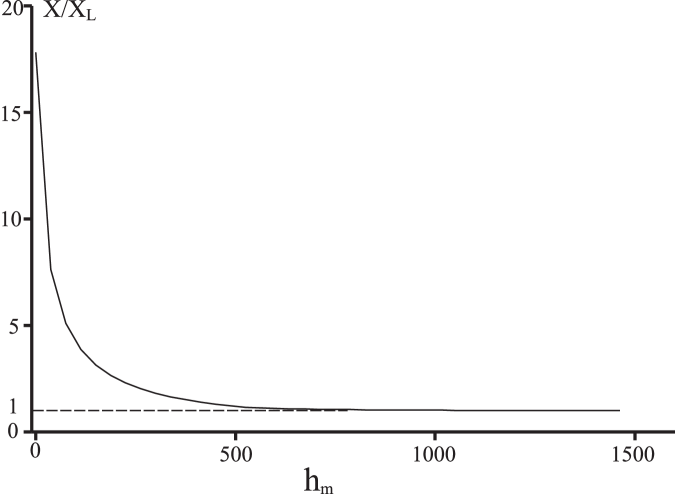
Figure 5: The surface reactance $X$ (in units of the reactance $X_{L}$ in the absence of the DC current) vs. dimensionless amplitude $h_{m}/\tilde{H}$ of the AC signal at $H=500{\tilde{H}}$.

VI Conclusion

Nonlinear interaction of electromagnetic waves with a strong DC transport current in a thin metal film leads to unusual physical effects due to specific, typical only for metals, magnetodynamic mechanism of nonlinearity. These effects have been studied by analyzing the nonlinear response of the film, which carries the DC current, irradiated bilaterally by electromagnetic wave. The interaction of the wave with the current results in nonanalytical behaviour of the AC electric field on the sample surface which is characterized by appearance of sharp kinks. The increase of the current is accompanied by a rise of the amplitude of oscillations of the electric field at the surface of the sample. This, in turn, causes to the growth of the imaginary part of the surface impedance of the conductor.

The results obtained in this treatment are valid under certain applicability conditions. Firstly, the AC electric field $\Delta{\cal E}(x,t)$ must be small comparing to the potential electric field $E_{0}(t)$. It follows from formulae (III), (40), and (41) that the quantities ${\cal E}$ and $\Delta{\cal E}_{m}$, Eq.(44), are of the same order. Therefore, to ascertain the restrictions imposed by the condition ${\cal E}\ll E_{0}(t)$, we can use quantity $\Delta{\cal E}_{m}$ in the latter condition. The quantity $\Delta{\cal E}_{m}$should be much less than the minimum value the function $E_{0}(t)$, i.e. the magnitude of potential field (34) for $\cos\omega t=0$. The desired inequality reads

$$d^{2}\frac{h_{m}l}{HR}\ll\delta^{2}_{n}(\omega),\qquad\delta^{2}_{n}(\omega)=\frac{c^{2}}{4\pi\sigma_{0}\omega},$$ (59)

where $\delta_{n}(\omega)$ represents the characteristic penetration depth of the AC field into a metal under the condition of normal skin effect. Secondly, the non-uniform component of magnetic field inside the film must necessarily be much less than $h_{m}$. This stems from the assumption that the AC magnetic field $h(x,t)$ should be quasi-uniform ($h(x,t)\simeq h_{m}\cos\omega t$) across the bulk of the film. The maximum value of the non-uniform correction can be estimated from the first of Maxwell’s equations (8) as $(4\pi\sigma_{tr}\Delta{\cal E}_{m}d/c)\sim h_{m}(d/\delta)^{2}$, where an effective penetration depth $\delta(\omega)$ equals to $\delta_{n}(\omega)(R/l)^{1/2}$. As a result, we come to a requirement of the quasi-uniform property of the AC magnetic field which can be written in the following form:

$$d^{2}\frac{l}{R}\ll\delta^{2}_{n}(\omega).$$ (60)

Comparing the restrictions imposed by inequalities (59) and (60), it can be seen that condition (59) is more strict at large AC amplitudes, $h_{m}>H$, while for small values of $h_{m}$ one should use inequality (60).

For a sample with thickness $d=10^{-3}$ cm, the electron free path $l=10^{-1}$ cm, the concentration of electron $N=10^{23}$ cm^-3, the Fermi momentum $p_{F}=10^{-19}$ g$\cdot$cm/sec and for magnetic fields $h_{m}=H=100$ Oe, we have $\omega<10^{5}$ sec^-1 using conditions (59) and (60). At such values of the parameters, conditions (59) and (60) are fulfilled as well as condition (5), which states that the value of the mean free path of electron should be large.

Unusual manifestation of specific magnetodynamic mechanism of nonlinearity discussed in the present paper calls for future investigation. In particular it would be very interesting to explore experimentally theoretical predictions made in this work.

References

- (1) Dolgopolov V T 1980 Sov. Phys. Usp. 23 134
- (2) Makarov N M and Yampol’skii V A 1991 Sov.J. Low Temp. Phys. 17 285
- (3) Babkin G I and Dolgopolov V T 1976 Solid State Commun. 18 713
- (4) Makarov N M and Yampol’skii V 1983 Sov. Phys.-JETP 58 357
- (5) Fisher L M, Voloshin I F, Makarov N M and Yampol’skii V A 1993 J. Phys.: Condens. Matter 5 8741
- (6) Kaner E A, Makarov N M, Yurkevich I V and Yampol’skii V 1987 Sov. Phys.-JETP 66 158
- (7) Vugalter G A and Demikhovskii V Ya 1976 Sov. Phys.-JETP 43 739
- (8) Skobov V G and Chernov A S 1996 Sov. Phys.-JETP 82 535
- (9) Fisher L M, Makarov N M, Vekslerchik V E and Yampol’skii V A 1995 J. Phys.: Condens. Matter 7 7549
- (10) Makarov N M, Tkachev G B and Vekslerchik V E 1998 J. Phys.: Condens. Matter 10 1033
- (11) Kaner E A, Makarov N M, Snapiro I B and Yampol’skii V A 1984 Sov. Phys.-JETP 60 1252
- (12) Fuchs K 1938 Proc. Cambr. Phil. Soc. 38 100
- (13) Voloshin I F, Kravchenko S V, Podlevskikh N A and Fisher L M 1985 Sov. Phys.-JETP 62 132