Conformal Dynamics of Fractal Growth Patterns Without Randomness

Abstract

Many models of fractal growth patterns (like Diffusion Limited Aggregation and Dielectric Breakdown Models) combine complex geometry with randomness; this double difficulty is a stumbling block to their elucidation. In this paper we introduce a wide class of fractal growth models with highly complex geometry but without any randomness in their growth rules. The models are defined in terms of deterministic itineraries of iterated conformal maps, automatically generating the function $\Phi^{(n)}(\omega)$ which maps the exterior of the unit circle to the exterior of an $n$-particle growing aggregate. The complexity of the evolving interfaces is fully contained in the deterministic dynamics of the conformal map $\Phi^{(n)}(\omega)$. We focus attention to a class of growth models in which the itinerary is quasiperiodic. Such itineraries can be approached via a series of rational approximants. The analytic power gained is used to introduce a scaling theory of the fractal growth patterns. We explain the mechanism for the fractality of the clusters and identify the exponent that determines the fractal dimension.

I Introduction

In this paper we introduce a new class of fractal growth patterns in two dimensions, constructed in terms of the conformal maps from the exterior of the unit circle to the exterior of the growing cluster. Until now most of the interesting fractal growth models included randomness as an essential aspect of the growth algorithms. Foremost in such models has been the diffusion limited aggregation (DLA) model that was introduced in 1981 by T. Witten and L. Sander [1]. This model has been shown to underlie many pattern forming processes including dielectric breakdown [2], two-fluid flow [3], and electro-chemical deposition [4]. The algorithm begins with fixing one particle at the center of coordinates in $d$-dimensions, and follows the creation of a cluster by releasing random walkers from infinity, allowing them to walk around until they hit any particle belonging to the cluster. Upon hitting they are attached to the growing cluster. The growth probability for a random walker to hit the interface is known as the “harmonic measure”, being the solution of the harmonic (Laplace) equation with the appropriate boundary conditions. The DLA model was generalized to a family of models known collectively as Dielectric Breakdown Models, in which the density of growth probability is the density of the harmonic measure raised to a power $\eta$ [5]. For $\eta=1$ one regains the DLA model; the interval $\eta\in(0,\infty)$ generates a family of growth patterns from compact to a single needle. For $\eta=0$ one obtains a growth probability that is uniform for all boundary points. This is known as the Eden model that was introduced originally to describe the growth of cancer cells [6].

The fundamental difficulty of all these models is that their mathematical description calls for solving equations with boundary conditions on a complex, evolving interface. It is therefore advantageous to swap for a simple boundary, like the unit circle, and to delegate the complexity to the dynamics of the conformal map from the exterior of the unit circle to the exterior of the growing cluster. For continuous time processes this method had been around for decades [7, 8], and had been used extensively. For discrete particle growth such a language was developed recently [9, 10, 11], showing that DLA in two dimensions can be grown by iterating stochastic conformal maps. In this paper we employ this new language to define models in which the stochasticity is eliminated altogether, to create deterministic iterations of conformal maps with very interesting fractal growth properties. It is stressed below that these new models and their interesting properties are natural extensions of the discrete conformal dynamics; it may be very difficult to study such models with the traditional techniques in physical space.

A central thesis of this paper is that the growth models introduced below are simpler to understand than DLA, even though the fractal geometry exhibited does not seem simpler. Indeed, we present below some tools and concepts that allow us to explain why the growing cluster is fractal. We present a scaling theory of the growing clusters, and identify the exponent that determines the fractal dimension. In sect. 2 we review the basic ideas of conformal dynamics as a method to grow DLA and related growth patterns. In Sec.3 we make the point that within this framework randomness can be eliminated from the discussion without changing the properties of the fractal growth: one can have deterministic growth rules with clusters that are indistinguishable from DLA. In Sec.4 we introduce fractal growth patterns that are obtained from quasiperiodic itineraries of iterated conformal maps. These itineraries are characterized by a winding number $W$. The growing clusters have complex geometries and a difference appearance for every $W$. We propose nevertheless that all the quadratic irrationals belong to the same universality class, and that the dimensions of their clusters are the same. In Sec.5 we consider rational approximants $P/Q$ to the quadratic irrational winding numbers $W$’s. With rational approximants the growth patterns crossover from a fractal phase of growth to a 1-dimensional star-like growth pattern. We argue that the analysis of the crossover as a function of $Q$ provides us with a scaling theory, allowing the introduction of universality classes and the achievement of data collapse. In Sec.6 we elucidate the mechanism for crossover from fractal to 1-dimensional growth, and identify the exponent that determines the fractal dimension. In Sec.7 we summarize and offer final remarks regarding the availability of a renormalization group treatment and of the road ahead.

II Discrete Conformal Dynamics for Fractal Growth Patterns

The basic idea is to follow the evolution of the conformal mapping $\Phi^{(n)}(w)$ which maps the exterior of the unit circle $e^{i\theta}$ in the mathematical $w$–plane onto the complement of the (simply-connected) cluster of $n$ particles in the physical $z$–plane [9, 10, 11]. The unit circle is mapped to the boundary of the cluster which is parametrized by the arc length $s$, $z(s)=\Phi^{(n)}(e^{i\theta})$. This map $\Phi^{(n)}(w)$ is made from compositions of elementary maps $\phi_{\lambda,\theta}$,

$$\Phi^{(n)}(w)=\Phi^{(n-1)}(\phi_{\lambda_{n},\theta_{n}}(w))\ ,$$ (1)

where the elementary map $\phi_{\lambda,\theta}$ transforms the unit circle to a circle with a “bump” of linear size $\sqrt{\lambda}$ around the point $w=e^{i\theta}$. Accordingly the map $\Phi^{(n)}(w)$ adds on a new bump to the image of the unit circle under $\Phi^{(n-1)}(w)$. The bumps in the $z$-plane simulate the accreted particles in the physical space formulation of the growth process. The main idea in this construction is to choose the positions of the bumps $\theta_{n}$ and their sizes $\sqrt{\lambda_{n}}$ such as to achieve accretion of fixed linear size bumps on the boundary of the growing cluster according to the growth rules appropriate for the particular growth model that we discuss.

As an example consider DLA. In $z$-space we want to accrete particles according to the harmonic measure. This means that the probability for the $n$th particle to hit a boundary element $ds$ equals $P(s)ds$, where $P(s)$ (the density of the harmonic measure [9, 10, 12]) and $ds$ are:

$$P(s) = \frac{1}{|{\Phi^{(n-1)}}^{{}^{\prime}}(e^{i\theta})|}\ ,$$ (2)

$$ds = |{\Phi^{(n-1)}}^{{}^{\prime}}(e^{i\theta})|d\theta\ .$$ (3)

Here $e^{i\theta}$ is the preimage of $z(s)$. Accordingly the probability to grow on an interval $d\theta$ is uniform (independent of $\theta$). Thus to grow a DLA we have to choose random positions $\theta_{n}$, and $\lambda_{n}$ in Eq.(1) according to

$$\lambda_{n}=\frac{\lambda_{0}}{|{\Phi^{(n-1)}}^{\prime}(e^{i\theta_{n}})|^{2}}\ .$$ (4)

This way we accrete fixed size bumps in the physical plane according to the harmonic measure. The elementary map $\phi_{\lambda,\theta}$ is chosen as [9]

$$\phi_{\lambda,0}(w)=w^{1-a}\left\{\frac{(1+\lambda)}{2w}(1+w)\right.$$ (5)

$$\left.\times\left[1+w+w\left(1+\frac{1}{w^{2}}-\frac{2}{w}\frac{1-\lambda}{1+\lambda}\right)^{1/2}\right]-1\right\}^{a}$$ (6)

$$\phi_{\lambda,\theta}(w)=e^{i\theta}\phi_{\lambda,0}(e^{-i\theta}w)\,,$$ (7)

The parameter $a$ is confined in the range $0<a<1$, determining the shape of the bump. We employ $a=2/3$ which is consistent with semicircular bumps. The recursive dynamics can be represented as iterations of the map $\phi_{\lambda_{n},\theta_{n}}(w)$,

$$\Phi^{(n)}(w)=\phi_{\lambda_{1},\theta_{1}}\circ\phi_{\lambda_{2},\theta_{2}}\circ\dots\circ\phi_{\lambda_{n},\theta_{n}}(\omega)\ .$$ (8)

The DLA cluster is fully determined by the stochastic itinerary $\{\theta_{i}\}_{i=1}^{n}$. In Fig. 1 we present a typical DLA cluster grown by this method to size $n=10^{5}$. The main point of this paper is that the same method can be now used to grow a large variety of interesting fractal shapes, but without any randomness in the growth algorithm.

III DLA-like clusters without randomness

As a first example of a new model we will remove the stochasticity of DLA, leaving the growth characteristics unchanged. To this aim consider an itinerary

$$\theta_{n+1}=2\theta_{n}~{}~{}{\rm mod}2\pi\ ,$$ (9)

together with Eq.(4). Such an itinerary, although deterministic, is chaotic (in fact Bernoulli, Kolmogorov and ergodic), covering the unit circle uniformly, with $\delta$-function correlation between consecutive $\theta$ values. Accordingly, we expect the growing cluster to be indistinguishable from a DLA, as is indeed the case, cf. Fig. 2.

One advantage of the present formalism is that such a statement can be made quantitatively, not by eyeball. The function $\Phi^{(n)}(w)$ and $\phi_{\lambda,\theta}(w)$ can be expanded in a Laurent series in which the highest power is $w$ [9, 10]:

$$\Phi^{(n)}(w)=F^{(n)}_{1}w+F^{(n)}_{0}+F^{(n)}_{-1}w^{-1}+F^{(n)}_{-2}w^{-2}+\dots$$ (10)

The recursion equations for the Laurent coefficients of $\Phi^{(n)}(w)$ can be obtained analytically, and in particular one shows that [9, 10]

$$F_{1}^{(n)}=\prod_{k=1}^{n}[1+\lambda_{k}]^{a}\,.$$ (11)

The importance of this lies in the fact that $F_{1}^{(n)}$ determines that fractal dimension of the cluster. Defining $R_{n}$ as the minimal radius of all circles in $z$ that contain the $n$-cluster, one can prove that [13]

$$R_{n}\leq 4F_{1}^{(n)}\ .$$ (12)

Accordingly one expects that

$$F^{(n)}_{1}\sim n^{1/D}\sqrt{\lambda_{0}}\ ,$$ (13)

as $\sqrt{\lambda_{0}}$ is the only length scale in the problem. We can thus present, as an example, plots of $F_{1}^{(n)}$ for our deterministic model (9) together with $F_{1}^{(n)}$ in any stochastic DLA growth, see Fig. 3. Another comparison is furnished by the statistics of $\lambda_{n}$. For the DLA case it was shown in [9, 10] that

$$\langle\lambda_{n}\rangle=\frac{1}{aDn}\ ,$$ (14)

where the average is taken over the harmonic measure. This is in agreement with the “electrostatic relation” derived by Halsey, [14]. In the Bernoulli itinerary there is no randomness and no probability measure, but we may still define a “running average” by, say, the last $M$ iterations

$$\langle\lambda_{n}\rangle_{M}\equiv\frac{1}{M}\sum_{k=n-M}^{n}\lambda_{k}\ .$$ (15)

In Fig. 4 we show a related quantity, $(\sum_{k=n-M}^{M}k\lambda_{k})/M$ for $M=1000$ and $M=10000$. We see that up to the expected fluctuations it settles down very quickly on the appropriate value of the DLA cluster, i.e. $1/aD=.877..$. Any other quantitative comparison that one can think of leads to the same conclusion, i.e the Bernoulli itinerary is a bona fide generic DLA. Of course, this is not surprising: the correlation properties of successive values of $\theta_{n}$ in (9) are indistinguishable from random numbers on the interval $[0,2\pi]$. Nevertheless, our point is that the present growth algorithm gives us freedom to choose deterministic itineraries resulting in DLA or other growth patterns, and we next exploit this freedom to explore new geometries.

IV Fractal Growth with quasi-periodic itineraries

A Winding numbers and geometry

A new class of models is obtained by using a quasi-periodic itinerary. Consider a simple map of the circle with a winding number W:

$$\theta_{i+1}=\theta_{i}+2\pi W\ .$$ (16)

If we choose $W$ rational, $W=P/Q$, then after a cross-over time the cluster grown is locked into a 1-dimensional object made of rays. In the next subsection we present an extensive discussion of the cross over time and of the properties of the 1-dimensional phase of growth. As an example consider in Fig. 5 the cluster resulting from (16) with $W=233/144$. On the other hand, for an irrational winding $W$ the itinerary is ergodic and the cluster grown is geometrically non-trivial. As a first example we present the case $W=\rho$ where $\rho$ is the Golden Mean, $\rho=(\sqrt{5}+1)/2$. The fractal cluster that is associated with this rule is shown in Fig.6. The cluster has a fractal dimension $D=1.86\pm 0.03$, as determined from the scaling of $F_{1}^{(n)}$. This is considerably higher than DLA (for which $D\approx 1.71$).

The golden mean is best approximated by the continued fraction representation

$$\rho=\frac{1}{1+\frac{1}{1+\frac{1}{1+\cdots}}}\ .$$ (17)

Such a continued fraction is denoted below as $[0,\bar{1}]$. It is known that the golden mean is special in presenting the slowest converging continued fraction. Other quadratic irrationals also have periodic continued fractions that converge faster. In Figs. 7-11 we show the clusters grown with $W=\sqrt{2},~{}\sqrt{3},~{}(1+\sqrt{10})/3,~{}(\sqrt{13}-1)/2$ and $\sqrt{7}$ respectively. The continued fraction representations of these winding numbers are $[1,\bar{2}],[1,\overline{1,2}],[\overline{1,2,1}],[1,\bar{3}],[2,\overline{1,1,1,4}]$ respectively. In choosing these examples we picked quadratic irrationals whose representations converge relatively slowly. This facilitates the exposition of scaling theory presented below.

We note that the clusters shown have very complicated geometry. Consider for example the cases $W=(\sqrt{13}-1)/2$ and $W=\sqrt{7}$ shown in Figs. 10, 11 respectively. They exhibit thin spiral growth patterns at their root, and then become bushy and thin in an apparently oscillatory fashion. Accordingly, it becomes unclear whether the different quadratic irrational winding numbers result in the same overall fractal dimension. This question warrants some extra analysis. We will argue below that in spite of the difference appearance and the oscillations in the “bushiness”, the clusters grown by quadratic irrational winding numbers have the same fractal dimension $D$.

B Different growth rules: period doubling itinerary

Clearly, one can come up with an arbitrary number of different growth rules. In this paper we will consider only one additional itinerary, to underline the fact that quadratic irrational windings lead to a class of their own. This itinerary is constructed such that after every $2^{n}$ iterations the points $\theta_{k}$ chosen on the circle are equidistributed without repetitions. The order of visitation is determined by the following rule:

$$\theta_{i} = 2\pi x_{i}\ ,$$ (18)

$$x_{i+1} = x_{i}+\frac{3}{2^{k_{i}+1}}-1$$ (19)

$$k_{i} = -[\log_{2}{(1-x_{i})}]\ ,$$ (20)

where $[\dots]$ stands for the integer value. We refer to this itinerary below as the “period doubling” algorithm. The cluster grown with this rule is shown in Fig. 12 . The dimension of this cluster is $D=1.77\pm 0.02$. In contrast to the quadratic irrationals in this case a comparison of $F_{1}^{(n)}$ of this cluster to $F_{1}^{(n)}$ of the golden mean itinerary shows a different scaling dependence on $n$ (cf. Fig. 13 ).

C Universality classes?

In the previous section we noted that the geometry of some of the clusters with quadratic irrational winding exhibit oscillations. It is thus not clear whether they have the same fractal dimension $D$. In this subsection we provide numerical test of the claim that the quadratic irrationals belong to the same universality class. In the the following sections we address this question using additional tools.

To study quantitatively the oscillatory fractal geometry we consider the dependence of $F_{1}^{(n)}$ on $n$. In Fig. 14 panel a we present compensated plots of $F_{1}^{(n)}(\sqrt{2})$ vs.$F_{1}^{(n)}(\sqrt{3})$ and vs. $F_{1}^{(n)}$ of a DLA as a function of $n$.

It appears that although this ratio exhibits oscillations, these are bounded and decreasing in amplitude, at least up to $n=10^{5}$. For comparison we show in panel b of Fig. 14 a plot of $F_{1}^{(n)}(\sqrt{2})/F_{1}^{(n)}(DLA)$. Here we see the clear difference in dimension as seen in the ratio approaching zero as a power law in $n$. In Fig. 15 we show compensated plots of $F_{1}^{(n)}$ of the clusters in Figs. 7-11 versus $F_{1}^{(n)}$ of the golden mean growth. We see oscillations on the logarithmic scale, but again these are bounded, and we propose that this points towards the possibility that all quadratic irrationals winding numbers lead to the same overall dimension of the cluster. In the next section we address the issue of universality classes using additional tools.

V Towards a scaling theory: winding with rational approximants

To gain understanding of the geometry of the clusters grown with quadratic irrational winding numbers we will make use now of the well known fact that these irrationals can be systematically approximated by rational approximants. Thus, having a cluster constructed with a golden mean itinerary, a natural question is what happens to the growth pattern when $\rho$ is replaced by ratios of successive Fibonacci numbers which are defined by the recursion relation $F_{m+1}=F_{m}+F_{m-1}$, $F_{0}=0$, $F_{1}=1$. Using rational approximants $\rho_{m}=F_{m-1}/F_{m}$, the itinerary becomes periodic on the unit circle with period $F_{m}$, and it is observed in simulations (see Fig. 5 ) that while for small clusters $n\ll n_{c}(F_{m})$ the cluster appears fractal, for $n\gg n_{c}(F_{m})$ the cluster consists of a set of $F_{m}$ rays, sometimes fused into a smaller set of 1-dimensional rays whose number is extremely sensitive to the initial conditions (here controlled by the value of $\lambda_{0}$).

A The 1-dimensional phase

The properties of the 1-dimensional phase are important for developing a scaling theory. As an example of the interesting behaviour seen as a function of $\lambda_{0}$ consider Fig. 16 in which clusters with $W=144/89$ are grown with 4 values of $\lambda_{0}$ which are 0.11, 0.22, 0.44, and 0.88. Evidently the cross over from fractal to 1-dimensional behaviour depends on $\lambda_{0}$. We also note that the number of rays in the 1-dimensional phase has a nonmonotonic dependence on $\lambda_{0}$. This indicates high sensitivity of the number of rays to changes in the initial conditions. Obviously, the radius of the cluster in the 1-dimensional case is inversely proportional to the number of rays. On the other hand, we have found a surprising invariant: $F_{1}^{(n)}$ is asymptotically invariant to the number of rays (i.e. to initial conditions) being always equal to $n\sqrt{\lambda_{0}}/Q$, up to a constant of proportionality depending on the microscopic parameter $a$ only. The numerical evidence is shown in Fig. 17. Note the convergence to the golden mean in panel a, and to $\sqrt{2}$ in panel b (which is the value of the ratios of $\sqrt{\lambda_{0}}$). This finding puts strict bounds on the number of possible rays. The upper bound is obviously $Q$. The lower bound stems from the inequality $R_{n}\leq 4F_{1}^{(n)}$, meaning that the number of rays must be larger than $Q/4$. This invariance also indicates that the geometry of the rays is not arbitrary, and that the angles between them are arranged to agree with an invariant $F_{1}^{(n)}$.

B Scaling Function

The crossover in fractal shape is a general result for any periodic itinerary with $W=P/Q$, and suggests the existence of a scaling for $F_{1}^{(n)}$ of the form

$$F_{1}^{(n)}=n^{1/D}\sqrt{\lambda_{0}}f(n^{1/\alpha}/Q),$$ (21)

where we have assumed that the crossover cluster size scales as

$$n_{c}(Q)\sim Q^{\alpha}.$$ (22)

The asymptotic forms of $F_{1}^{(n)}$ obey $F_{1}^{(n)}\sim n^{1/D}\sqrt{\lambda_{0}}$ for $n\ll n_{c}(Q)$, while $F_{1}^{(n)}\sim(n/Q)\sqrt{\lambda_{0}}$ for $n\gg n_{c}(Q)$. In the first asymptote we expect $D$ to be the same for all values of rational approximants to $\rho$, including the limiting fractal cluster. The growing cluster cannot distinguish between the rational approximant and the limiting irrational as long as the fractal phase is observed. The second asymptote is demonstrated in the previous subsection. Thus we require that the asymptotic forms of the scaling function obey

$$f(u) \rightarrow f(0)\mbox{~{}as~{}$u\rightarrow 0$}\ ,$$ (23)

$$f(u) \sim u\mbox{~{}as~{}$u\rightarrow\infty$}\ .$$ (24)

The second asymptote (24) determines the scaling relation

$$\alpha=D/(D-1)\ .$$ (25)

For the Golden Mean fractal $D\approx 1.86$ and consequently in this case $\alpha\approx 2.16$.

In Fig. 18 $F_{1}^{(n)}/(n^{1/D}\sqrt{\lambda_{0}})$ is plotted against the scaling variable $u=n^{1/\alpha}/Q$ for six different clusters with different values of $W$ and $\lambda_{0}$. The best data collapse was obtained using the value $\alpha=2.15$ The data collapse achieved is readily apparent with the scaling function $f(u)$ predicted by the theory.

VI The crossover and the estimate of the dimension

In this section we discuss the properties of the conformal map $\phi_{\lambda,\theta}$ which determine the cross over from fractal to 1-dimensional growth. In other words, we will attempt to provide an independent estimate of $n_{c}$ as a function of the winding number $W$. If we succeeded to estimate the exponent $\alpha$ in (22) independently from Eq.(25), we would have an equation for the dimension.

To understand the crossover, we note that the reason for the fractal growth phase with rational winding is that after every event of growth the interface $z(e^{i\theta})$ is non-locally reparametrized in addition to the local growth event. Accordingly, a periodic orbit on the unit circle is not necessarily mapped to a periodic orbit in $z$. The region in the unit circle which is significantly affected by growing the $n$th bump has a scale $\sqrt{\lambda_{n}}$ centered around $\theta_{n}$ [15]. Accordingly we can estimate when reparametrization will cause a “miss” in the mapped orbit: as long as

$$\sqrt{\lambda_{n}}\geq\frac{2\pi}{Q}\ ,$$ (26)

the growth will remain fractal. We can therefore expect a crossover to 1-dimensional growth when this condition is violated, something that is bound to happen since typical values of $\lambda_{n}$ are expected to decreases with $n$, cf. Eq.(14) and the discussion below.

What remains is to estimate $\lambda_{n}$ as a function of $n$ in the cross over region that is defined by

$$\sqrt{\lambda_{n_{c}}}\approx 2\pi/Q\ .$$ (27)

In the fractal region $\lambda_{n}$ is a highly erratic function of $n$. Even though we do not have here randomness in the sense of DLA, it is natural to consider, in a fashion similar to Eq.(15), the distribution of $\lambda_{k}$ over $Q$ successive steps of growth. For $Q$ large enough such distributions have well defined moments. In particular consider the first moment

$$\langle\lambda_{n}\rangle_{Q}\equiv\frac{1}{Q}\sum_{k=n-Q}^{n}\lambda_{k}$$ (28)

The power law dependence of $F_{1}^{(n)}$ and Eq.(11) imply that this moment has to be

$$\langle\lambda_{n}\rangle_{Q}=\frac{1}{anD}\ .$$ (29)

If we estimate $\lambda_{n_{c}}$ in Eq. (27) by its mean (29), we would write

$$\lambda_{n_{c}}\sim 1/n_{c}~{}~{}\rightarrow~{}~{}n_{C}\sim Q^{2}.$$ (30)

Thus $D/(D-1)=2$ or $D=2$. Even though we get an overestimate, this is a good indication that we are on the right track. The reason for the overestimate is that we neglected the fluctuations that sometime lead to $\lambda_{n}$ much larger than the mean. We expect a cross over to occur when the largest $\sqrt{\lambda_{k}}$ are smaller than $2\pi/Q^{2}$, since it is enough to have a few large $\lambda_{k}$ to cause a reparametrization that will ruin a potential periodic orbit. We thus seek a condition

$$\lambda_{n}^{\rm max}\equiv{\rm max}\{\lambda_{k}\}_{k=n-Q}^{n}\approx\frac{4\pi^{2}}{Q^{2}}\ .$$ (31)

We note that $\lambda_{k}$ is an erratic function of $k$, and therefore the condition (31) can be met more than once in a given series $\lambda_{k}$. In Fig. 19 we show two log-log plots of $n_{c}$ computed from the value of $n$ for which $\sqrt{\lambda_{n}^{\rm max}}=2\pi/Q$, plotted as a function of $Q=F_{m}$. The cross over value $n_{c}$ was computed in two different ways. In circles we exhibit the values obtained from measuring when $\sqrt{\lambda_{n}^{\rm max}}=2\pi/Q$ for the first time, and in squares we exhibit the values obtained from $\sqrt{\lambda_{n}^{\rm max}}=2\pi/Q$ for the last time. Computing the slopes by linear regression and averaging between them we find the scaling law

$$n_{c}\sim Q^{2.17\pm 0.03}\ .$$ (32)

Comparing with Eqs.(22), (25) we get an estimate for $D=1.86\pm 0.03$, in excellent agreement with the determination of the dimension by $F_{1}^{(n)}$.

We note in passing that $\lambda_{n}^{\rm max}$ can be assigned a generalized dimension $D_{\infty}$ in the language of Hentschel and Procaccia [16]. Define

$$\langle\lambda_{n}^{q}\rangle_{Q}\equiv\frac{1}{Q}\sum_{k=n-Q}^{n}\lambda^{q}_{k}\ .$$ (33)

From [10] the precise scaling law is

$$\lambda_{n}^{\rm max}=\lim_{q\to\infty}\langle\lambda_{n}^{q}\rangle_{Q}^{1/q}\sim n^{-2D_{\infty}/D}\ .$$ (34)

Comparing with (25) we conclude that in this case there exists a scaling relation

$$D_{\infty}=D-1\ .$$ (35)

Such a scaling relation was conjectured by Turkevich and Scher for DLA [17] (of course with a different $D$ and $D_{\infty}$). While there are severe doubts about the correctness of this conjecture for DLA[14], we point out that in our case it follows directly from elementary considerations.

A The period doubling itinerary

Even though the period doubling itinerary leads to a cluster whose fractal dimension differs from the quadratic irrational windings, we show here that the ideas presented above pertain equally to this growth pattern. Instead of rational approximants we use here, naturally, $2^{n}$-periodic orbits which are obtained by cutting the itinerary (20) after $2^{n}$ iterations and repeating it periodically. The crossover from fractal to 1-dimensional growth is seen also in this case, and we can use it in a very similar way to identify the crucial exponent that determines the dimension of the asymptotic cluster. Indeed, the whole set of ideas developed above repeats verbatim by changing $Q$ with $2^{n}$. What remains is to find $\lambda_{n}^{\rm max}$ as a function of $n$. In Fig .20 we show the data collapse obtained as in Fig. 18 for the quasiperiodic analog. We show nine different data sets with periodic itineraries of periods 32, 64 and 128 and $\sqrt{\lambda_{0}}$ values of 0.22, 0.44 and 0.88. The scaling function for these data sets is plotted as a function of $u=n^{.44}/Q$, where the exponent is computed from $D=1.78$. It is noteworthy that the scaling function obtained appears identical to the scaling function $f(u)$ for the quasiperiodic family. For comparison we added in Fig .20 also one curve from the quasiperiodic class, and it appears indistinguishable from the rest.

The conclusion from this data collapse is that the mechanism governing the crossover from fractal to 1-dimensional growth phases here is the same as the one discussed above for the quasiperiodic itineraries. The difference between the dimensions of the period doubling cluster and the quasiperiodic cluster must lie in the different numerical value of the exponent characterizing $\lambda_{n}^{\rm max}$ as a function of $n$. In this case the natural averaging cycles are of length $Q=2^{n}$. Fig. 21 is the analog of Fig. 19 for the period doubling itinerary, where the critical value $n_{c}$ was estimated from the first time that $\sqrt{\lambda_{n}^{\rm max}}$ became smaller than $2\pi/2^{n}$.

The linear regression provides us with the the scaling law

$$n_{c}\sim Q^{2.33\pm 0.1}\ .$$ (36)

Computing $D$ we find $D=1.75\pm 0.05$ in good agreement with the numerical estimate from $F_{1}^{(n)}$.

VII Summary and the road ahead

The main points of this paper are as follows:

• The iterated conformal maps algorithm for fractal growth patterns offers a convenient way to introduce a large number of deterministic growth models with highly non-trivial fractal geometry.

• Itineraries with irrational winding numbers generate fractal growth patterns. We proposed that all the quadratic irrationals produce clusters of the same fractal dimension, in spite of different appearance.

• By considering a series of rational approximants we could produce a scaling theory of the growing clusters, achieving data collapse for all values of $n,\lambda_{0}$ and $P/Q$.

• Identifying the mechanism for the cross over from fractal to 1-dimensional growth phases we could pinpoint the exponent that determines the fractal dimension $D$. This exponent characterizes the $n$ dependence of the extremal values of $\lambda_{n}$.

• The mechanism appears general; itineraries leading to different cluster dimensions, like the period doubling itinerary (20) and its truncated versions, can be understood in the same way. The scaling function (21) and the scaling relation (25) are general, but the exponent $\alpha$ changes. Its determination by the scaling of $\lambda_{n}^{\rm max}$ Eq.(31) is however general.

We note that all the numerical tests point out in favour of this scenario, and in our opinion rule out a value $D=2$ for the clusters discussed above. The only way to get 2-dimensional growth, as shown above, is if the distribution of $\lambda_{n}$ does not multiscale, i.e. all $D_{q}$ are the same, and the scaling of $\lambda_{n}^{\rm max}$ identifies with the scaling of the average of $\lambda_{n}$.

Nevertheless, we point out that the crucial step in our scenario, the determination of the exponent $\alpha$ in Eq.(22), was achieved numerically. The scaling theory presented above has a strong flavour of a renormalization group approach. It appears that such an underlying theory may have a low codimension, maybe with 1 important exponent, the one characterizing the rate of crossover of the rational approximants to the irrational limit. The search of such a theory appears to be an important task for the near future.

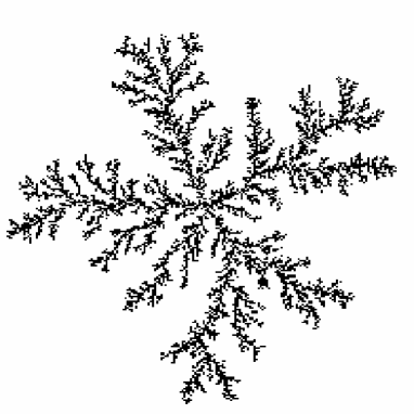
FIG. 1.: A DLA cluster, $n=10^{5}$.

FIG. 2.: A Bernoulli cluster, $n=10^{5}$.

FIG. 3.: Comparison of $F_{1}^{(n)}$ for a DLA (continuous line) and a Bernoulli itinerary (dashed line).

FIG. 4.: The average of $k\lambda_{k}$ over the last $M$ iterations of the Bernoulli itinerary, with $M=10^{3}$ (continuous line) and $M=10^{4}$ (dashed line). The horizontal line is the expected value, $1/aD$. The fluctuations are typical, reflecting the multi-scaling distributions of $\lambda_{k}$ in which large deviations are highly probable.

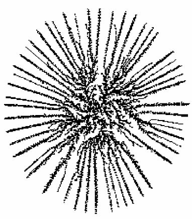
FIG. 5.: Cluster grown with $W=233/144$ to $n=10^{4}$. Note the crossover from fractal to 1-dimensional growth phases

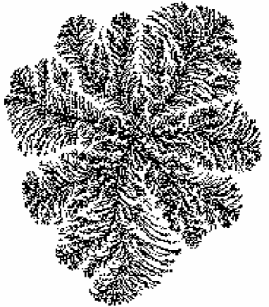
FIG. 6.: The cluster grown with $W=\rho$ to $n=10^{5}$

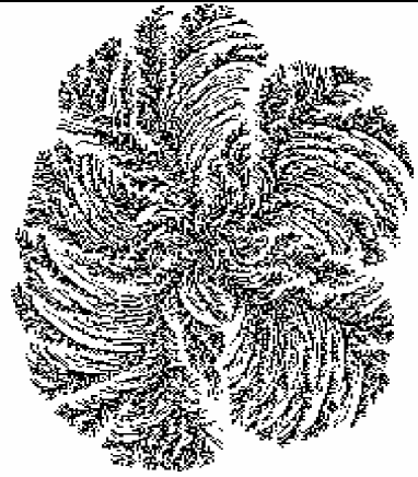
FIG. 7.: The cluster grown with $W=2^{1/2}$ to $n=10^{5}$

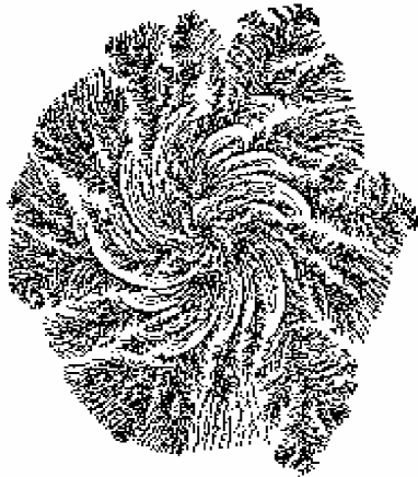
FIG. 8.: The cluster grown with $W=3^{1/2}$ to $n=10^{5}$

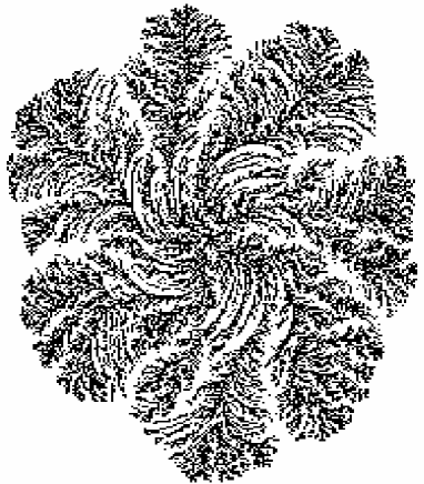
FIG. 9.: The cluster grown with $W=(1+(10)^{1/2})/3$ to $n=10^{5}$

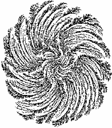
FIG. 10.: The cluster grown with $W=((13)^{1/2}-1)/2$ to $n=10^{5}$

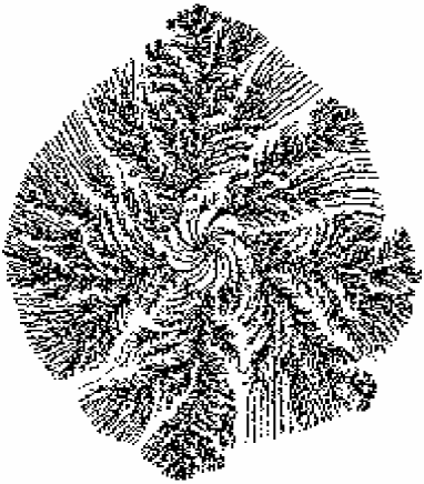
FIG. 11.: The cluster grown with $W=7^{1/2}$ to $n=10^{5}$

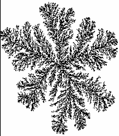
FIG. 12.: The cluster grown with the period doubling itinerary to $n=10^{5}$

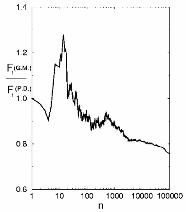
FIG. 13.: The ratio between $F_{1}^{(n)}$ of the golden mean and period doubling clusters.

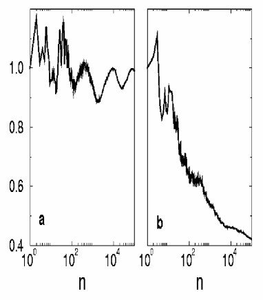
FIG. 14.: Panel a: The ratio between of $F_{1}^{(n)}$ of the clusters grown with $W=2^{1/2}$ and $W=3^{1/2}$. Panel b: The ratio between of $F_{1}^{(n)}$ of the cluster grown with $W=2^{1/2}$ and a typical DLA

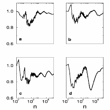
FIG. 15.: The ratio between of $F_{1}^{(n)}$ of the golden mean and other quadratic irrationals. Panels a-d show respectively $W=2^{1/2}$, $W=(1+(10)^{1/2})/3$ , $W((13^{1/2}-1)/2)$ and $W=7^{1/2}$

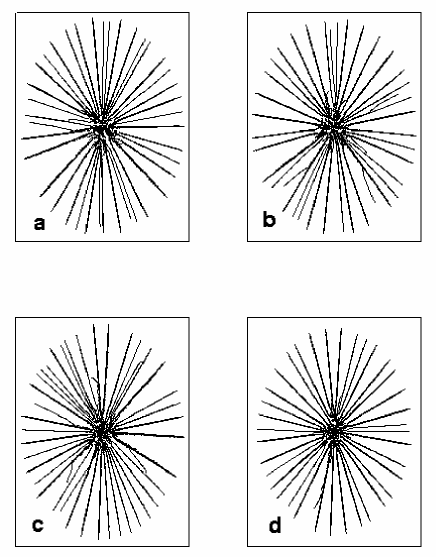
FIG. 16.: Clusters grown with $W=144/89$ with four different values of $\lambda_{0}$, from 0.11 to 0.88.

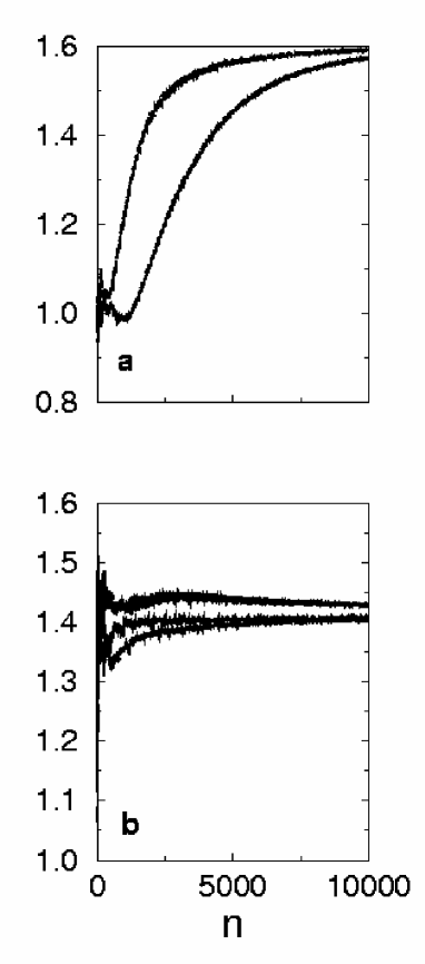
FIG. 17.: Panel a: The ratio of $F_{1}^{(n)}$ for clusters grown with $\lambda_{0}=0.88$, and winding numbers $W=89/55$ and $W=144/89$ (upper curve) and $W=144/89$ and $W=233/144$) (lower curve). Both converge to the golden mean. Panel b: Similar plots with $W=144/89$. $\lambda_{0}=0.22$ is compensated by $\lambda_{0}=0.11$, 0.44 by 0.22 and 0.88 by 0.44. All these plots converge to $2^{1/2}$.

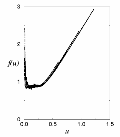
FIG. 18.: Scaling behaviour for six separate data sets for $f(u)$ with $u=n^{.46}/Q$. Shown are $\lambda 0=0.88$ with $W=89/55$, $W=144/89$, $W=233/144$, $W=377/233$, $\lambda 0=0.44$ with $W=144/89$, $\lambda 0=0.22$ with $W=144/89$.

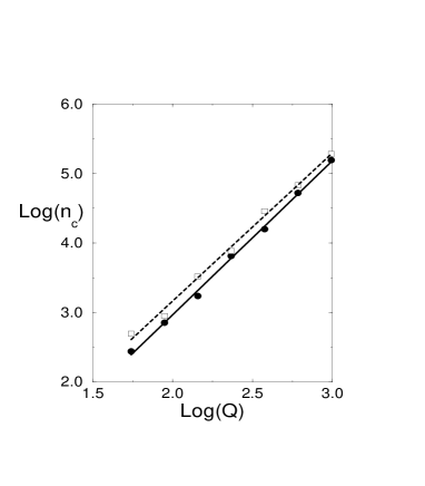
FIG. 19.: The measured the cross over values $n_{c}$ as a function of $Q$ in a log-log plots. In dots are the values of $n$ for which the condition $\lambda_{n}^{\rm max}=4\pi^{2}/Q^{2}$ was met for the first time, in squares for the last time.

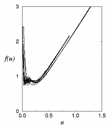
FIG. 20.: Scaling behaviour for nine separate data sets for clusters grown with truncated period doubling itineraries, in addition to one data set of the quasiperiodic class. See text for details

FIG. 21.: The measured the cross over values $n_{c}$ as a function of $Q=2^{n}$ in a log-log plot. Shown are the values of $n$ for which the condition $\lambda_{n}^{\rm max}=(2\pi/2^{n})^{2}$ was met for the first time.

- [1] T.A. Witten and L.M. Sander, Phys. Rev. Lett, 47, 1400 (1981).
- [2] L. Niemeyer, L. Pietronero and H.J. Wiessmann, Phys. Rev. Lett. 52, 1033 (1984).
- [3] L. Paterson, Phys. Rev. Lett. 52, 1621 (1984).
- [4] R. M. Brady and R. C. Ball, Nature 309, 225 (1984); D. Grier, E. Ben-Jacob, R. Clarke, and L. M. Sander, Phys. Rev. Lett. 56, 1264 (1986)
- [5] A. Erzan, L. Pietronero, A. Vespignani, Rev.Mod.Phys. 67, 545 (1995).
- [6] P. Meakin, in Phase Transitions and Critical Phenomena, eds. C. Domb and J. L. Lebowitz, Vol.12 (Academic, NY, 1988).
- [7] P.G. Saffman and G.I. Taylor, Proc. Roy. Soc. London Series A, 245,312 (1958).
- [8] B. Shraiman and D. Bensimon, Phys.Rev. A30, 2840 (1984).
- [9] M. B. Hastings and L. S. Levitov, Physica D 116, 244 (1998).
- [10] B. Davidovich, H.G.E. Hentschel, Z. Olami, I.Procaccia, L. M. Sander, and E. Somfai, Phys. Rev. E, 59 1368 (1999)
- [11] B. Davidovich and I. Procaccia, Euro. Phys. Lett, 48, 547 (1999)
- [12] T.C. Halsey, P. Meakin and I. Procaccia, Phys. Rev. Lett. 56, 854 (1986).
- [13] P. L. Duren, Univalent Functions, (Springer-Verlag, New York, 1983).
- [14] T.C. Halsey, Phys. Rev. Lett. 59, 2067 (1987).
- [15] T.C. Halsey, Phys.Rev.Lett. 72 1228 (1994).
- [16] H.G.E. Hentschel and I. Procaccia, Physica D 8, 435 (1983).
- [17] L.A. Turkevich and H. Scher, Phys. Rev. Lett. 55, 1026 (1985).