Paraxial propagation of a quantum charge
in a random magnetic field

Abstract

The paraxial (parabolic) theory of a near forward scattering of a quantum charged particle by a static magnetic field is presented. From the paraxial solution to the Aharonov-Bohm scattering problem the transverse transfered momentum (the Lorentz force) is found. Multiple scattering is considered for two models: (i) Gaussian $\delta$-correlated random magnetic field; (ii) a random array of the Aharonov-Bohm magnetic flux line. The paraxial gauge-invariant two-particle Green function averaged with respect to the random magnetic field is found by an exact evaluation of the Feynman integral. It is shown that in spite of the anomalous character of the forward scattering, the transport properties can be described by the Boltzmann equation. The Landau quantization in the gauge field of the Aharonov-Bohm lines is discussed.

I Introduction

The paper addresses the problem of quantum transport of a charge in an inhomogeneous static random magnetic field. In recent years, this or related problems have been met in a number of contexts in physics of 2-dimensional systems. For instance, in the composite fermion model of the Fractional Quantum Hall Effect, a (fictitious) random magnetic field is the environment which controls dynamics of effective charge carriers [2]. One meets the fluctuating gauge fields in some models of high temperature superconductors [3], where the gauge field is the tool to impose the constrain of no double occupancy in the $t-J$ model [4]. Besides, stochastically inhomogeneous magnetic field can be experimentally created by various ways. For example, the field is irregular near the surface of a superconductor in an external magnetic field if the Abrikosov flux lattice is disordered; depending on the experimental conditions, the magnetic field inhomogeneities may be weak and smooth, or the field may be concentrated in an irregular array of flux tubes. Various aspects of transport in the magnetic field of the Abrikosov vortices, the weak localization in particular, have been studied in Refs. [5, 6, 7, 8, 9, 10, 11]. In recent years, the random magnetic field problem has been an active subject area Refs. [12, 13, 14, 15, 16, 17, 18, 19, 20].

The formulation of the problem is as follows. A particle with the electric charge $e$ and the mass $m$ moves on the $x-y$ plane subject to a vector potential potential $\mathchoice{{\hbox{\boldmath$\displaystyle A$}}}{{\hbox{\boldmath$\textstyle A$}}}{{\hbox{\boldmath$\scriptstyle A$}}}{{\hbox{\boldmath$\scriptscriptstyle A$}}}(A_{x},A_{y})$ generated by a magnetic field $b(x,y)=\left(\mathchoice{{\hbox{\boldmath$\displaystyle{\rm rot\,}A$}}}{{\hbox{\boldmath$\textstyle{\rm rot\,}A$}}}{{\hbox{\boldmath$\scriptstyle{\rm rot\,}A$}}}{{\hbox{\boldmath$\scriptscriptstyle{\rm rot\,}A$}}}\right)_{z}$. Two random fields models are considered in the paper. In the first one, the magnetic field $b(\mathchoice{{\hbox{\boldmath$\displaystyle r$}}}{{\hbox{\boldmath$\textstyle r$}}}{{\hbox{\boldmath$\scriptstyle r$}}}{{\hbox{\boldmath$\scriptscriptstyle r$}}})$ is a random Gaussian variable with zero average, $\langle b\rangle=0$, specified by the correlator

$$\langle b(\mathchoice{{\hbox{\boldmath$\displaystyle r$}}}{{\hbox{\boldmath$\textstyle r$}}}{{\hbox{\boldmath$\scriptstyle r$}}}{{\hbox{\boldmath$\scriptscriptstyle r$}}})b(\mathchoice{{\hbox{\boldmath$\displaystyle r$}}}{{\hbox{\boldmath$\textstyle r$}}}{{\hbox{\boldmath$\scriptstyle r$}}}{{\hbox{\boldmath$\scriptscriptstyle r$}}}^{\prime})\rangle=\left({\Phi_{0}\over{2\pi}}\right)^{2}{1\over{{\cal L}^{2}}}\delta(\mathchoice{{\hbox{\boldmath$\displaystyle r$}}}{{\hbox{\boldmath$\textstyle r$}}}{{\hbox{\boldmath$\scriptstyle r$}}}{{\hbox{\boldmath$\scriptscriptstyle r$}}}-\mathchoice{{\hbox{\boldmath$\displaystyle r$}}}{{\hbox{\boldmath$\textstyle r$}}}{{\hbox{\boldmath$\scriptstyle r$}}}{{\hbox{\boldmath$\scriptscriptstyle r$}}}^{\prime})\ ,$$ (1)

where $\Phi_{0}={hc\over e}$ is the flux quantum; the strength of the random magnetic field is characterized via the length ${\cal L}$ the meaning of which is that the magnetic flux through the area ${\cal L}^{2}$ is typically of order of $\Phi_{0}$. The random field is assumed to be weak in the sense that ${\cal L}$ much exceeds the wave length $\lambdabar\equiv\hbar/p$, $p$ being the particle momentum. In another model [21, 22, 23] which is motivated by fractional statistics theories, the gauge potential is created by a random array of the Aharonov-Bohm flux lines. A system of the Abrikosov vortices (e.g. in the gate of a MOSFET transistor [5, 6, 7]) may serve as an experimental realization of the Aharonov-Bohm array if the particle wave length much exceeds the vortex (magnetic) size.

In the random magnetic field case, the traditional approach of the theory of disordered systems [24] meets difficulties on the very first steps. Indeed, the simplest object that is the single particle Green’s function $G(1,2)=\langle\psi(\mathchoice{{\hbox{\boldmath$\displaystyle r$}}}{{\hbox{\boldmath$\textstyle r$}}}{{\hbox{\boldmath$\scriptstyle r$}}}{{\hbox{\boldmath$\scriptscriptstyle r$}}}_{1})\psi^{*}(\mathchoice{{\hbox{\boldmath$\displaystyle r$}}}{{\hbox{\boldmath$\textstyle r$}}}{{\hbox{\boldmath$\scriptstyle r$}}}{{\hbox{\boldmath$\scriptscriptstyle r$}}}_{2})\rangle$, is not gauge invariant and the physical meaning of its averaging with respect to the vector potential $\textstyle A$ generated by the random field is not clear. One may define a gauge invariant combination $\tilde{G}(1,2)=\langle\psi(\mathchoice{{\hbox{\boldmath$\displaystyle r$}}}{{\hbox{\boldmath$\textstyle r$}}}{{\hbox{\boldmath$\scriptstyle r$}}}{{\hbox{\boldmath$\scriptscriptstyle r$}}}_{1})\psi^{*}(\mathchoice{{\hbox{\boldmath$\displaystyle r$}}}{{\hbox{\boldmath$\textstyle r$}}}{{\hbox{\boldmath$\scriptstyle r$}}}{{\hbox{\boldmath$\scriptscriptstyle r$}}}_{2})\rangle\exp[i{e\hbar\over c}\int_{{\cal C}_{12}}d\mathchoice{{\hbox{\boldmath$\displaystyle l\cdot A$}}}{{\hbox{\boldmath$\textstyle l\cdot A$}}}{{\hbox{\boldmath$\scriptstyle l\cdot A$}}}{{\hbox{\boldmath$\scriptscriptstyle l\cdot A$}}}]$ where the path ${\cal C}_{12}$ connects the points $\mathchoice{{\hbox{\boldmath$\displaystyle r$}}}{{\hbox{\boldmath$\textstyle r$}}}{{\hbox{\boldmath$\scriptstyle r$}}}{{\hbox{\boldmath$\scriptscriptstyle r$}}}_{1}$ and $\mathchoice{{\hbox{\boldmath$\displaystyle r$}}}{{\hbox{\boldmath$\textstyle r$}}}{{\hbox{\boldmath$\scriptstyle r$}}}{{\hbox{\boldmath$\scriptscriptstyle r$}}}_{2}$. Albeit gauge independent, $\tilde{G}(1,2)$ essentially depends on the choice of the path ${\cal C}_{12}$. With the point $\mathchoice{{\hbox{\boldmath$\displaystyle r$}}}{{\hbox{\boldmath$\textstyle r$}}}{{\hbox{\boldmath$\scriptstyle r$}}}{{\hbox{\boldmath$\scriptscriptstyle r$}}}_{1,2}$ connected by the straight line, the field averaged $\tilde{G}(1,2)$ has been found in Ref.[12].

Another problem is the diverging scattering rate ${1\over\tau}$. For small scattering angles $\phi$, the differential cross-section behaves like ${1\over\phi^{2}}$ so that the scattering total cross-section is infinite. In other words, the life time of a state with the definite momentum is zero. The conventional diagram technique [24] where ${\hbar\over\tau}$ is assumed to be small compared with the kinetic energy, becomes questionable. On the other hand, it is known [25] that in gauge-invariant response functions the self energy enters in combination with the vertex corrections and the divergence cancels out. In Ref.[15], it has been attempted to introduce a physically sensible gauge-invariant “single-particle time” $\tau$ as a parameter entering the Landau level broadening.

The main purpose of this paper is to develop a scheme which allows one to study the most singular part of interaction with random magnetic field, that is the near forward scattering.

To pinpoint the physics behind the theoretical difficulties, consider first propagation of a plane wave. It is common in wave mechanics to analyze propagation in terms of wave fronts, i.e. the surfaces (lines in 2D) of constant phase. The property of the wave front line is that the probability current is locally perpendicular to the line. In the magnetic field, the phase of the wave function is ill-defined because of the gauge freedom. Nevertheless, one can construct a gauge invariant quantity $\chi$ defined on a line, which in a limited sense plays the role of the phase: Given the wave function $\psi(\mathchoice{{\hbox{\boldmath$\displaystyle r$}}}{{\hbox{\boldmath$\textstyle r$}}}{{\hbox{\boldmath$\scriptstyle r$}}}{{\hbox{\boldmath$\scriptscriptstyle r$}}})$ and the vector potential $\textstyle A$, the phase $\chi(\mathchoice{{\hbox{\boldmath$\displaystyle s$}}}{{\hbox{\boldmath$\textstyle s$}}}{{\hbox{\boldmath$\scriptstyle s$}}}{{\hbox{\boldmath$\scriptscriptstyle s$}}})$ for the points $\textstyle s$ on a line $S$ is defined through its differential as

$$d\chi={m\over\hbar|\psi|^{2}}\mathchoice{{\hbox{\boldmath$\displaystyle j\cdot$}}}{{\hbox{\boldmath$\textstyle j\cdot$}}}{{\hbox{\boldmath$\scriptstyle j\cdot$}}}{{\hbox{\boldmath$\scriptscriptstyle j\cdot$}}}d\mathchoice{{\hbox{\boldmath$\displaystyle s$}}}{{\hbox{\boldmath$\textstyle s$}}}{{\hbox{\boldmath$\scriptstyle s$}}}{{\hbox{\boldmath$\scriptscriptstyle s$}}}$$ (2)

where $\mathchoice{{\hbox{\boldmath$\displaystyle j$}}}{{\hbox{\boldmath$\textstyle j$}}}{{\hbox{\boldmath$\scriptstyle j$}}}{{\hbox{\boldmath$\scriptscriptstyle j$}}}={1\over m}\Re\left(\psi^{*}\left({\hbar\over i}\mathchoice{{\hbox{\boldmath$\displaystyle\nabla$}}}{{\hbox{\boldmath$\textstyle\nabla$}}}{{\hbox{\boldmath$\scriptstyle\nabla$}}}{{\hbox{\boldmath$\scriptscriptstyle\nabla$}}}-{e\over c}\mathchoice{{\hbox{\boldmath$\displaystyle A$}}}{{\hbox{\boldmath$\textstyle A$}}}{{\hbox{\boldmath$\scriptstyle A$}}}{{\hbox{\boldmath$\scriptscriptstyle A$}}}\right)\psi\right)$ is the probability current density. Provided the line $S$ does not have self-intersections, $\chi$ is an unique function of $\textstyle s$.

If $\chi$ is a constant, i.e. $\mathchoice{{\hbox{\boldmath$\displaystyle j\cdot$}}}{{\hbox{\boldmath$\textstyle j\cdot$}}}{{\hbox{\boldmath$\scriptstyle j\cdot$}}}{{\hbox{\boldmath$\scriptscriptstyle j\cdot$}}}d\mathchoice{{\hbox{\boldmath$\displaystyle s$}}}{{\hbox{\boldmath$\textstyle s$}}}{{\hbox{\boldmath$\scriptstyle s$}}}{{\hbox{\boldmath$\scriptscriptstyle s$}}}=0$ and $\mathchoice{{\hbox{\boldmath$\displaystyle j$}}}{{\hbox{\boldmath$\textstyle j$}}}{{\hbox{\boldmath$\scriptstyle j$}}}{{\hbox{\boldmath$\scriptscriptstyle j$}}}\perp d\mathchoice{{\hbox{\boldmath$\displaystyle s$}}}{{\hbox{\boldmath$\textstyle s$}}}{{\hbox{\boldmath$\scriptstyle s$}}}{{\hbox{\boldmath$\scriptscriptstyle s$}}}$, the local current and the normal to $S$ are parallel, so that $S$ is a wave front. If $\chi$ is a slowly varying function, $\lambdabar\left(\chi(\mathchoice{{\hbox{\boldmath$\displaystyle s$}}}{{\hbox{\boldmath$\textstyle s$}}}{{\hbox{\boldmath$\scriptstyle s$}}}{{\hbox{\boldmath$\scriptscriptstyle s$}}})-\chi(\mathchoice{{\hbox{\boldmath$\displaystyle 0$}}}{{\hbox{\boldmath$\textstyle 0$}}}{{\hbox{\boldmath$\scriptstyle 0$}}}{{\hbox{\boldmath$\scriptscriptstyle 0$}}})\right)$ gives the local distance from $S$ to the wave front passing through the point $\mathchoice{{\hbox{\boldmath$\displaystyle s$}}}{{\hbox{\boldmath$\textstyle s$}}}{{\hbox{\boldmath$\scriptstyle s$}}}{{\hbox{\boldmath$\scriptscriptstyle s$}}}=0$.

                               

(a)                                                                             (b)

FIG. 1.: The wave front of a wave on a plane. (a) The wave front $S$ is a line at each point of which the probability current is directed perpendicular to the line. The gauge invariant phase $\chi$ is a constant along a wave front. On a general line $S$, chosen as a straight line in (b), the phase a function of the coordinate along the line $\textstyle s$. Its variation is found from Eq.(2). The physical meaning of $\chi(\mathchoice{{\hbox{\boldmath$\displaystyle s$}}}{{\hbox{\boldmath$\textstyle s$}}}{{\hbox{\boldmath$\scriptstyle s$}}}{{\hbox{\boldmath$\scriptscriptstyle s$}}})$ is that the phase difference $\Delta\chi(\mathchoice{{\hbox{\boldmath$\displaystyle s$}}}{{\hbox{\boldmath$\textstyle s$}}}{{\hbox{\boldmath$\scriptstyle s$}}}{{\hbox{\boldmath$\scriptscriptstyle s$}}})\equiv\left(\chi(\mathchoice{{\hbox{\boldmath$\displaystyle s$}}}{{\hbox{\boldmath$\textstyle s$}}}{{\hbox{\boldmath$\scriptstyle s$}}}{{\hbox{\boldmath$\scriptscriptstyle s$}}})-\chi(\mathchoice{{\hbox{\boldmath$\displaystyle 0$}}}{{\hbox{\boldmath$\textstyle 0$}}}{{\hbox{\boldmath$\scriptstyle 0$}}}{{\hbox{\boldmath$\scriptscriptstyle 0$}}})\right)$ multiplied by the wave length $\lambdabar$ shows the local distance $\lambdabar\Delta\chi$ from the line $S$ to the wave front.

Consider now how the random magnetic field affects the wave front upon its propagation. Take a state $\psi$, for which the line $x=0$ is a wave front corresponding to the propagation in the positive $x$-direction ($j_{x}$ ¿0). To satisfy the requirement $d\chi=0$, the wave function is

$\displaystyle\psi(x=0,y)=\exp\left[i{e\hbar\over c}\int\limits_{-\infty}^{y}dy\;A_{y}(x=0,y)\right]\;,$along the wave front $x=0$ (choice of lower limit of integration is not important).

To find the profile of the wave front having advanced from $x=0$ to a finite $x$, one can apply the usual eikonal-type approximation where the field affects only the phase of the wave function through the factor $\exp[{ie\over\hbar c}\int d\mathchoice{{\hbox{\boldmath$\displaystyle l\cdot A$}}}{{\hbox{\boldmath$\textstyle l\cdot A$}}}{{\hbox{\boldmath$\scriptstyle l\cdot A$}}}{{\hbox{\boldmath$\scriptscriptstyle l\cdot A$}}}]$, $d\mathchoice{{\hbox{\boldmath$\displaystyle l$}}}{{\hbox{\boldmath$\textstyle l$}}}{{\hbox{\boldmath$\scriptstyle l$}}}{{\hbox{\boldmath$\scriptscriptstyle l$}}}\parallel\hat{x}$ being along the direction of propagation:

$\displaystyle\psi(x,y)=\exp\left[{i\over{\hbar}}\left(px+{e\over c}\int\limits_{-\infty}^{y}dy\;A_{y}(0,y)+{e\over c}\int\limits_{0}^{x}dx\;A_{x}(x,y)\right)\right]\;.$Integrating Eq.(2), one finds the phase $\chi(y;x)$ as a function of $y$ for fixed $x$. For the phase difference $\Delta\chi(y_{1},y_{2};x)=\chi(y_{2};x)-\chi(y_{1};x)$, one gets after simple calculations:

$$\Delta\chi(y_{1},y_{2};x)=2\pi{\Phi(y_{1},y_{2};x)\over\Phi_{0}}$$ (3)

where $\Phi(y_{1},y_{2};x)$ is the magnetic flux through the area enclosed by the path $(0,y_{1})\rightarrow(0,y_{2})\rightarrow(x,y_{2})\rightarrow(x,y_{1})\rightarrow(0,y_{1})$ (see fig. 2).

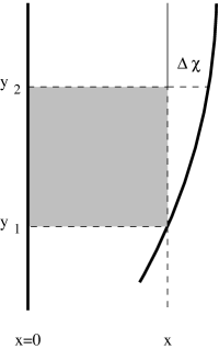
FIG. 2.: Propagation of the wave front magnetic field. As discussed in the text, one constructs a state for which the straight line at $x=0$ is a wave front. For a finite $x$, the profile of the front passing via the point $x,y_{1}$ is controlled by the phase difference $\Delta\chi=\chi(y_{2};x)-\chi(y_{1};z)$. The difference is proportional to the magnetic flux through through the shaded area.

A non-local character of the interaction with magnetic filed is clearly seen from Eq.(3): the phase difference is controlled by the flux rather than the magnetic field in the vicinity of the particle trajectories. The non-locality is obviously of the Aharonov-Bohm type.

Averaging with respect of the random magnetic field Eq.(1), one gets the variation of the phase difference

$\displaystyle(\Delta\chi)^{2}(y_{1},y_{2};x)={1\over 2}{|x|\cdot|y_{1}-y_{2}|\over{\cal L}^{2}}\;.$Most notable feature here is that $(\Delta\chi)^{2}$ grows with the separation $|y_{1}-y_{2}|$ (cf. Ref.[12]). For points separated by the distance $\Delta y$, the random phase difference is of order of $1$ when the wave front advances to $\Delta x\sim{\cal L}^{2}/\Delta y$. One sees that an infinite plane wave, for which $\Delta y\rightarrow\infty$, looses its coherence immediately, whatever small is the propagation distance $\Delta x$. (See Section V for a more formal derivation.) These qualitative arguments explain the actual meaning of the zero life time and show that it is not an artifact arising e.g. due to a violation of the gauge invariance.

To handle the anomalously intensive forward scattering, one needs a method suitable for a nonperturbative analysis of the small-angle multiple scattering. For this, the paraxial (parabolic) approximation [26] to the Schrödinger equation is chosen in the paper. The paraxial theory is applicable when the particle moves mainly in the direction of an “axis” and the momentum transverse to the axis remains always small. The paraxial approximation to the wave equation is most popular in optics where it gives a convenient description of light beams propagating in optical systems, their diffraction, focusing etc [27]. Taking scattering and diffraction broadening on equal footing, the paraxial approximation is more generally applicable then the eikonal one [28].

To make the paper self-contained, the derivation of the paraxial approximation is outlined in Sect.II. The case of magnetic field is considered in Sect.II A where a scheme for description of scattering by magnetic field is suggested. The scheme is in a sense gauge invariant, gauge freedom revealing itself only in the overall phases. As a limiting case, one recovers the well-known eikonal approximation (see Sect. II B).

To illustrate usage of the paraxial approximation, a simple problem of scattering of a charged particle by the Aharonov-Bohm magnetic flux line is considered in Sect.III. This (or equivalent) problem is of interest in a broad variety of contexts extending from the cosmic string theory [29] to superfluids [30, 31, 32] (the Iordanskii force) and superconductors [33] where the scattering of excitations by quantized vortex lines controls the vortex dynamics. Although the exact solution to the scattering problem has been known since the original paper of Aharonov and Bohm [34] (see also review [35] and references therein), certain controversy in the analysis and the interpretation of the solution still remains. Different opinions exist in the literature about the existence of the transverse force exerted by the Aharonov-Bohm line or a superfluid vortex. On the basis of the left-right symmetry in the Aharonov-Bohm differential cross-section, the authors of Refs. [36] and Ref.[37] have come to the conclusion that the line does not exert any Lorentz-like force (translated as the Iordanskii force in a superfluid). Other authors, [32, 21, 23, 38, 39] predict a finite force. Due to its simplicity, the paraxial solution allows one to perform a detailed analysis and resolve the controversy.

It is shown in In Sect.IV, that the paraxial scattering theory becomes manifestly gauge invariant if formulated in terms of by-linear in $\psi$ and $\psi^{*}$ object that is the density matrix $\rho$. The evolution of the density matrix is given by a gauge invariant two-particle Green function.

As discussed in Sect.IV A, the paraxial 2D stationary equation with inhomogeneous magnetic field can be written as a non-stationary 1D Schrödinger equation for a particle in a time-dependent electric field. This mapping allows one to present stationary solutions to the 2D magnetic field problem as the Feynman path integral for the effective 1D problem.

In Sect.V, the paraxial theory is applied to the model of $\delta$-correlated random magnetic field. It turns out to be possible to evaluate the Feynman path integral and by this to find a (paraxially) exact expression for the two-particle Green’s function averaged with respect to the magnetic field fluctuations. It is shown that the density matrix evolution can be mapped to the Boltzmann kinetic equation.

In Sect.VI, another model is considered where the random gauge filed is generated by a random array of Aharonov-Bohm fluxes. The flux lines are randomly distributed in the plane, the flux of a line, $\Phi$, is distributed with the probability $p(\Phi)$. The Aharonov-Bohm array may create an effective magnetic field $\tilde{B}$ if $p(\Phi)$ is asymmetric, $p(\Phi)\neq p(-\Phi)$.

In Sect.VI A, the Boltzmann equation for charge subject to a Gaussian random magnetic field or field of AB-array is derived. With the help of the Boltzmann equation, the resistivity tensor is found. Finally, in Sect.VI B we discuss the density of states of the levels due to the quantization of motion in the field $\tilde{B}$.

The results are summarized in Section VII

II Paraxial approximation

The paraxial approximation allows one to construct a family of solutions to the Schrödinger equation which are close to to the plane wave with a certain momentum $\mathchoice{{\hbox{\boldmath$\displaystyle p$}}}{{\hbox{\boldmath$\textstyle p$}}}{{\hbox{\boldmath$\scriptstyle p$}}}{{\hbox{\boldmath$\scriptscriptstyle p$}}}_{0}$. The wave function $\Psi_{Sch}$, a solution to the stationary Schrödinger equation, is presented as

$$\Psi_{Sch}(\mathchoice{{\hbox{\boldmath$\displaystyle r$}}}{{\hbox{\boldmath$\textstyle r$}}}{{\hbox{\boldmath$\scriptstyle r$}}}{{\hbox{\boldmath$\scriptscriptstyle r$}}})=\Psi(\mathchoice{{\hbox{\boldmath$\displaystyle r$}}}{{\hbox{\boldmath$\textstyle r$}}}{{\hbox{\boldmath$\scriptstyle r$}}}{{\hbox{\boldmath$\scriptscriptstyle r$}}})e^{{i\over{\hbar}}\mathchoice{{\hbox{\boldmath$\displaystyle p$}}}{{\hbox{\boldmath$\textstyle p$}}}{{\hbox{\boldmath$\scriptstyle p$}}}{{\hbox{\boldmath$\scriptscriptstyle p$}}}_{0}\mathchoice{{\hbox{\boldmath$\displaystyle\cdot r$}}}{{\hbox{\boldmath$\textstyle\cdot r$}}}{{\hbox{\boldmath$\scriptstyle\cdot r$}}}{{\hbox{\boldmath$\scriptscriptstyle\cdot r$}}}}\ ,$$ (4)

where the envelope paraxial function $\Psi(\mathchoice{{\hbox{\boldmath$\displaystyle r$}}}{{\hbox{\boldmath$\textstyle r$}}}{{\hbox{\boldmath$\scriptstyle r$}}}{{\hbox{\boldmath$\scriptscriptstyle r$}}})$ is supposed to be slowly varying at the distances of order of the wave length $\lambdabar={\hbar\over{p_{0}}}$.

The Schrödinger equation reads

$$\left(E(\hat{\mathchoice{{\hbox{\boldmath$\displaystyle p$}}}{{\hbox{\boldmath$\textstyle p$}}}{{\hbox{\boldmath$\scriptstyle p$}}}{{\hbox{\boldmath$\scriptscriptstyle p$}}}})+U\right)\Psi_{Sch}=E\Psi_{Sch}$$ (5)

$E(\mathchoice{{\hbox{\boldmath$\displaystyle p$}}}{{\hbox{\boldmath$\textstyle p$}}}{{\hbox{\boldmath$\scriptstyle p$}}}{{\hbox{\boldmath$\scriptscriptstyle p$}}})={1\over{2m}}\mathchoice{{\hbox{\boldmath$\displaystyle p$}}}{{\hbox{\boldmath$\textstyle p$}}}{{\hbox{\boldmath$\scriptstyle p$}}}{{\hbox{\boldmath$\scriptscriptstyle p$}}}^{2}$ and $U(\mathchoice{{\hbox{\boldmath$\displaystyle r$}}}{{\hbox{\boldmath$\textstyle r$}}}{{\hbox{\boldmath$\scriptstyle r$}}}{{\hbox{\boldmath$\scriptscriptstyle r$}}})$ being the kinetic and potential energy respectively. Given $\mathchoice{{\hbox{\boldmath$\displaystyle p$}}}{{\hbox{\boldmath$\textstyle p$}}}{{\hbox{\boldmath$\scriptstyle p$}}}{{\hbox{\boldmath$\scriptscriptstyle p$}}}_{0}$, the family of solutions in Eq.(4) corresponds to the eigen-energy $E=E(\mathchoice{{\hbox{\boldmath$\displaystyle p$}}}{{\hbox{\boldmath$\textstyle p$}}}{{\hbox{\boldmath$\scriptstyle p$}}}{{\hbox{\boldmath$\scriptscriptstyle p$}}}_{0})$ and the velocity $\mathchoice{{\hbox{\boldmath$\displaystyle v$}}}{{\hbox{\boldmath$\textstyle v$}}}{{\hbox{\boldmath$\scriptstyle v$}}}{{\hbox{\boldmath$\scriptscriptstyle v$}}}={\partial E(\mathchoice{{\hbox{\boldmath$\displaystyle p$}}}{{\hbox{\boldmath$\textstyle p$}}}{{\hbox{\boldmath$\scriptstyle p$}}}{{\hbox{\boldmath$\scriptscriptstyle p$}}}_{0})\over{\partial\mathchoice{{\hbox{\boldmath$\displaystyle p$}}}{{\hbox{\boldmath$\textstyle p$}}}{{\hbox{\boldmath$\scriptstyle p$}}}{{\hbox{\boldmath$\scriptscriptstyle p$}}}_{0}}}$. Inserting Eq.(4) into Eq.(5), one gets equation for $\Psi$,

$\displaystyle\Big{(}\widetilde{E}\big{(}\hat{\mathchoice{{\hbox{\boldmath$\displaystyle p$}}}{{\hbox{\boldmath$\textstyle p$}}}{{\hbox{\boldmath$\scriptstyle p$}}}{{\hbox{\boldmath$\scriptscriptstyle p$}}}}\big{)}-E(\mathchoice{{\hbox{\boldmath$\displaystyle p$}}}{{\hbox{\boldmath$\textstyle p$}}}{{\hbox{\boldmath$\scriptstyle p$}}}{{\hbox{\boldmath$\scriptscriptstyle p$}}}_{0})+U\Big{)}\Psi=0\;\;,\;\;\widetilde{E}\big{(}\hat{\mathchoice{{\hbox{\boldmath$\displaystyle p$}}}{{\hbox{\boldmath$\textstyle p$}}}{{\hbox{\boldmath$\scriptstyle p$}}}{{\hbox{\boldmath$\scriptscriptstyle p$}}}}\big{)}\equiv e^{-{i\over{\hbar}}\mathchoice{{\hbox{\boldmath$\displaystyle p$}}}{{\hbox{\boldmath$\textstyle p$}}}{{\hbox{\boldmath$\scriptstyle p$}}}{{\hbox{\boldmath$\scriptscriptstyle p$}}}_{0}\mathchoice{{\hbox{\boldmath$\displaystyle\cdot r$}}}{{\hbox{\boldmath$\textstyle\cdot r$}}}{{\hbox{\boldmath$\scriptstyle\cdot r$}}}{{\hbox{\boldmath$\scriptscriptstyle\cdot r$}}}}E\big{(}\hat{\mathchoice{{\hbox{\boldmath$\displaystyle p$}}}{{\hbox{\boldmath$\textstyle p$}}}{{\hbox{\boldmath$\scriptstyle p$}}}{{\hbox{\boldmath$\scriptscriptstyle p$}}}}\big{)}e^{{i\over{\hbar}}\mathchoice{{\hbox{\boldmath$\displaystyle p$}}}{{\hbox{\boldmath$\textstyle p$}}}{{\hbox{\boldmath$\scriptstyle p$}}}{{\hbox{\boldmath$\scriptscriptstyle p$}}}_{0}\mathchoice{{\hbox{\boldmath$\displaystyle\cdot r$}}}{{\hbox{\boldmath$\textstyle\cdot r$}}}{{\hbox{\boldmath$\scriptstyle\cdot r$}}}{{\hbox{\boldmath$\scriptscriptstyle\cdot r$}}}}\;,$which is still exact. The operator $\widetilde{E}(\hat{\mathchoice{{\hbox{\boldmath$\displaystyle p$}}}{{\hbox{\boldmath$\textstyle p$}}}{{\hbox{\boldmath$\scriptstyle p$}}}{{\hbox{\boldmath$\scriptscriptstyle p$}}}})=E(\mathchoice{{\hbox{\boldmath$\displaystyle p$}}}{{\hbox{\boldmath$\textstyle p$}}}{{\hbox{\boldmath$\scriptstyle p$}}}{{\hbox{\boldmath$\scriptscriptstyle p$}}}_{0}+{\hbar\over{i}}\mathchoice{{\hbox{\boldmath$\displaystyle\nabla$}}}{{\hbox{\boldmath$\textstyle\nabla$}}}{{\hbox{\boldmath$\scriptstyle\nabla$}}}{{\hbox{\boldmath$\scriptscriptstyle\nabla$}}})$ acting on the slowly varying function $\Psi$ is approximated in the paraxial theory as

$\displaystyle\widetilde{E}(\hat{\mathchoice{{\hbox{\boldmath$\displaystyle p$}}}{{\hbox{\boldmath$\textstyle p$}}}{{\hbox{\boldmath$\scriptstyle p$}}}{{\hbox{\boldmath$\scriptscriptstyle p$}}}})\approx E(\mathchoice{{\hbox{\boldmath$\displaystyle p$}}}{{\hbox{\boldmath$\textstyle p$}}}{{\hbox{\boldmath$\scriptstyle p$}}}{{\hbox{\boldmath$\scriptscriptstyle p$}}}_{0})+{\hbar\over{i}}\mathchoice{{\hbox{\boldmath$\displaystyle v$}}}{{\hbox{\boldmath$\textstyle v$}}}{{\hbox{\boldmath$\scriptstyle v$}}}{{\hbox{\boldmath$\scriptscriptstyle v$}}}\mathchoice{{\hbox{\boldmath$\displaystyle\cdot\nabla$}}}{{\hbox{\boldmath$\textstyle\cdot\nabla$}}}{{\hbox{\boldmath$\scriptstyle\cdot\nabla$}}}{{\hbox{\boldmath$\scriptscriptstyle\cdot\nabla$}}}+{1\over{2m}}\left({\hbar\over{i}}\mathchoice{{\hbox{\boldmath$\displaystyle\nabla$}}}{{\hbox{\boldmath$\textstyle\nabla$}}}{{\hbox{\boldmath$\scriptstyle\nabla$}}}{{\hbox{\boldmath$\scriptscriptstyle\nabla$}}}_{\perp}\right)^{2}\;,$here $\mathchoice{{\hbox{\boldmath$\displaystyle\nabla$}}}{{\hbox{\boldmath$\textstyle\nabla$}}}{{\hbox{\boldmath$\scriptstyle\nabla$}}}{{\hbox{\boldmath$\scriptscriptstyle\nabla$}}}_{\perp}$ denotes the gradient in the direction perpendicular to $\textstyle v$.

The paraxial approximation to the Schrödinger equation reads

$$\left(i\hbar\mathchoice{{\hbox{\boldmath$\displaystyle v$}}}{{\hbox{\boldmath$\textstyle v$}}}{{\hbox{\boldmath$\scriptstyle v$}}}{{\hbox{\boldmath$\scriptscriptstyle v$}}}\mathchoice{{\hbox{\boldmath$\displaystyle\cdot\nabla$}}}{{\hbox{\boldmath$\textstyle\cdot\nabla$}}}{{\hbox{\boldmath$\scriptstyle\cdot\nabla$}}}{{\hbox{\boldmath$\scriptscriptstyle\cdot\nabla$}}}+{\hbar^{2}\over{2m}}\mathchoice{{\hbox{\boldmath$\displaystyle\nabla$}}}{{\hbox{\boldmath$\textstyle\nabla$}}}{{\hbox{\boldmath$\scriptstyle\nabla$}}}{{\hbox{\boldmath$\scriptscriptstyle\nabla$}}}_{\perp}^{2}-U\right)\Psi=0\;.$$ (6)

(Condition of applicability are discussed later). The main feature of the paraxial approximation Eq.(6), is that it is of first order differential equation relative to the coordinate in the direction of the propagation $x=\mathchoice{{\hbox{\boldmath$\displaystyle r\cdot v$}}}{{\hbox{\boldmath$\textstyle r\cdot v$}}}{{\hbox{\boldmath$\scriptstyle r\cdot v$}}}{{\hbox{\boldmath$\scriptscriptstyle r\cdot v$}}}/v$.

Introducing formally “time” $\tau=x/v$, Eq.(6) takes the form, of the time dependent Schrödinger equation in a reduced space dimension:

$$i\hbar{\partial\over{\partial\tau}}\Psi=\left(-{\hbar^{2}\over{2m}}\mathchoice{{\hbox{\boldmath$\displaystyle\nabla$}}}{{\hbox{\boldmath$\textstyle\nabla$}}}{{\hbox{\boldmath$\scriptstyle\nabla$}}}{{\hbox{\boldmath$\scriptscriptstyle\nabla$}}}_{\perp}^{2}+U\right)\Psi\ ,$$ (7)

This formal analogy allows one to discuss the stationary solutions in terms of the wave moving in the direction $\textstyle v$, and call $x$ the current coordinate of the wave. The Feynman path integral equivalent to Eq.(7) gives an alternative method of solving the equation.

The probability current $\textstyle J$ is derived from the standard expression $\mathchoice{{\hbox{\boldmath$\displaystyle J$}}}{{\hbox{\boldmath$\textstyle J$}}}{{\hbox{\boldmath$\scriptstyle J$}}}{{\hbox{\boldmath$\scriptscriptstyle J$}}}={\hbar\over{m}}\Im\Psi_{Sch}^{*}\mathchoice{{\hbox{\boldmath$\displaystyle\nabla$}}}{{\hbox{\boldmath$\textstyle\nabla$}}}{{\hbox{\boldmath$\scriptstyle\nabla$}}}{{\hbox{\boldmath$\scriptscriptstyle\nabla$}}}\Psi_{Sch}$ and the definition Eq.(4). In the main approximation, the components parallel, $\mathchoice{{\hbox{\boldmath$\displaystyle J$}}}{{\hbox{\boldmath$\textstyle J$}}}{{\hbox{\boldmath$\scriptstyle J$}}}{{\hbox{\boldmath$\scriptscriptstyle J$}}}_{||}$, and perpendicular, $\mathchoice{{\hbox{\boldmath$\displaystyle J$}}}{{\hbox{\boldmath$\textstyle J$}}}{{\hbox{\boldmath$\scriptstyle J$}}}{{\hbox{\boldmath$\scriptscriptstyle J$}}}_{\perp}$, relative to $\textstyle v$, are

$$\mathchoice{{\hbox{\boldmath$\displaystyle J$}}}{{\hbox{\boldmath$\textstyle J$}}}{{\hbox{\boldmath$\scriptstyle J$}}}{{\hbox{\boldmath$\scriptscriptstyle J$}}}_{||}=\mathchoice{{\hbox{\boldmath$\displaystyle v$}}}{{\hbox{\boldmath$\textstyle v$}}}{{\hbox{\boldmath$\scriptstyle v$}}}{{\hbox{\boldmath$\scriptscriptstyle v$}}}|\Psi|^{2}\;\;,\;\;\mathchoice{{\hbox{\boldmath$\displaystyle J$}}}{{\hbox{\boldmath$\textstyle J$}}}{{\hbox{\boldmath$\scriptstyle J$}}}{{\hbox{\boldmath$\scriptscriptstyle J$}}}_{\perp}={\hbar\over{m}}\Im\Psi^{*}\mathchoice{{\hbox{\boldmath$\displaystyle\nabla$}}}{{\hbox{\boldmath$\textstyle\nabla$}}}{{\hbox{\boldmath$\scriptstyle\nabla$}}}{{\hbox{\boldmath$\scriptscriptstyle\nabla$}}}_{\perp}\Psi\ .$$ (8)

These expressions are consistent with the current conservation and Eq.(6) or Eq.(7): Indeed, the continuity equation which follows from Eq.(7),

$${\partial|\Psi|^{2}\over{\partial\tau}}+\text{{\bf div }}\mathchoice{{\hbox{\boldmath$\displaystyle J$}}}{{\hbox{\boldmath$\textstyle J$}}}{{\hbox{\boldmath$\scriptstyle J$}}}{{\hbox{\boldmath$\scriptscriptstyle J$}}}_{\perp}=0$$ (9)

is equivalent to $\text{div }\mathchoice{{\hbox{\boldmath$\displaystyle J$}}}{{\hbox{\boldmath$\textstyle J$}}}{{\hbox{\boldmath$\scriptstyle J$}}}{{\hbox{\boldmath$\scriptscriptstyle J$}}}=0$ with $\textstyle J$ from Eq.(8). The continuity in Eq.(9) means that the paraxial wave function can be normalized:

$\displaystyle\int d\mathchoice{{\hbox{\boldmath$\displaystyle r$}}}{{\hbox{\boldmath$\textstyle r$}}}{{\hbox{\boldmath$\scriptstyle r$}}}{{\hbox{\boldmath$\scriptscriptstyle r$}}}_{\perp}|\Psi|^{2}=1$fixing the total flux in the beam to $\textstyle v$.

The required solution to the paraxial equation can be chosen by imposing a proper boundary condition to Eq.(6) (“initial” condition in the case of Eq.(7))

a Paraxial approximation: conditions of applicability

The paraxial theory is based on the approximation $E(\mathchoice{{\hbox{\boldmath$\displaystyle p$}}}{{\hbox{\boldmath$\textstyle p$}}}{{\hbox{\boldmath$\scriptstyle p$}}}{{\hbox{\boldmath$\scriptscriptstyle p$}}})-E(\mathchoice{{\hbox{\boldmath$\displaystyle p$}}}{{\hbox{\boldmath$\textstyle p$}}}{{\hbox{\boldmath$\scriptstyle p$}}}{{\hbox{\boldmath$\scriptscriptstyle p$}}}_{0})\approx v\delta p_{||}+{1\over{2m}}(\delta\mathchoice{{\hbox{\boldmath$\displaystyle p$}}}{{\hbox{\boldmath$\textstyle p$}}}{{\hbox{\boldmath$\scriptstyle p$}}}{{\hbox{\boldmath$\scriptscriptstyle p$}}}_{\perp})^{2}$, $\delta\mathchoice{{\hbox{\boldmath$\displaystyle p$}}}{{\hbox{\boldmath$\textstyle p$}}}{{\hbox{\boldmath$\scriptstyle p$}}}{{\hbox{\boldmath$\scriptscriptstyle p$}}}\equiv\mathchoice{{\hbox{\boldmath$\displaystyle p$}}}{{\hbox{\boldmath$\textstyle p$}}}{{\hbox{\boldmath$\scriptstyle p$}}}{{\hbox{\boldmath$\scriptscriptstyle p$}}}-\mathchoice{{\hbox{\boldmath$\displaystyle p$}}}{{\hbox{\boldmath$\textstyle p$}}}{{\hbox{\boldmath$\scriptstyle p$}}}{{\hbox{\boldmath$\scriptscriptstyle p$}}}_{0}$ where the term ${1\over{2m}}(\delta\mathchoice{{\hbox{\boldmath$\displaystyle p$}}}{{\hbox{\boldmath$\textstyle p$}}}{{\hbox{\boldmath$\scriptstyle p$}}}{{\hbox{\boldmath$\scriptscriptstyle p$}}}_{||})^{2}$ is neglected. This is justifiable if the angle, $\theta\sim{\delta p_{\perp}\over{p_{0}}}$, between $\textstyle p$ and $\mathchoice{{\hbox{\boldmath$\displaystyle p$}}}{{\hbox{\boldmath$\textstyle p$}}}{{\hbox{\boldmath$\scriptstyle p$}}}{{\hbox{\boldmath$\scriptscriptstyle p$}}}_{0}$ is small, $\theta\ll 1$. If the motion is free, $\delta p_{\perp}\sim{\hbar\over{w}}$ where $w$ is the width of the beam (defined by the boundary conditions). Paraxial approximation is therefore applicable if the beam is wide in the scale of the wave length $\lambdabar$,

$$w\sim{\delta p_{\perp}\over p_{0}}\gg\lambdabar\ .$$ (10)

The scattering by the potential $U$ changes the angle by $\theta_{\text{scat}}\sim U/E$ . The paraxial approximation requires the small angle scattering to be dominant, $\theta\sim\theta_{\text{scat}}\ll 1$, so that the theory is applicable only for fast particles: $E\gg|U|$. It is important however, that, as in the case of the eikonal approximation [28], the theory is applicable beyond the Born approximation: the phase shift $\delta\varphi\sim{Ua\over{\hbar v}}\sim{U\over{E}}{pa\over{\hbar}}$, $a$ being the thickness of the layer where $U\neq 0$, may be large even for fast particles.

Unlike the eikonal approximation where only the phase variations are taken into account, the paraxial theory allows also for the change of the profile of the beam, i.e. $|\Psi(\mathchoice{{\hbox{\boldmath$\displaystyle r$}}}{{\hbox{\boldmath$\textstyle r$}}}{{\hbox{\boldmath$\scriptstyle r$}}}{{\hbox{\boldmath$\scriptscriptstyle r$}}})|$ due to diffraction (or, equivalently, to broadening of the wave packet in the language of Eq.(7)). If $w$ is a typical size of the transverse structure defined by either the initial condition or scattering, the “diffraction blurring of the image” happens when the beam travels the distance $x_{\text{diff}}$,

$$x_{\text{diff}}\sim{w^{2}\over{\lambdabar}}\ .$$ (11)

The diffraction length $x_{\text{diff}}$ is the typical distance for the paraxial approximation while region $x\ll x_{\text{diff}}$ is described by the eikonal approximation.

Applicability of the approximation at large distances requires further analysis. The paraxial relation $\delta p_{||}=-{1\over{2p_{0}}}(\delta\mathchoice{{\hbox{\boldmath$\displaystyle p$}}}{{\hbox{\boldmath$\textstyle p$}}}{{\hbox{\boldmath$\scriptstyle p$}}}{{\hbox{\boldmath$\scriptscriptstyle p$}}}_{\perp})^{2}$ is valid up to a small correction $(\delta p_{||})_{2}$ due to the neglected quadratic term: $(\delta p_{||})_{2}\simeq{1\over{2p_{0}}}(\delta p_{||})^{2}$. In the main approximation, $(\delta p_{||})_{2}\sim p_{\perp}^{4}/{p_{0}^{3}}$. Although small in comparison with $\delta p_{||}$, the correction is important at long enough distances; it can be ignored only if ${(\delta p_{||})_{2}x/{\hbar}}<1$. Thus, the paraxial approximation is reliable if the distance traveled by the beam is not not too large,

$$x<{w^{4}\over{\lambdabar^{3}}}\sim\left({w\over{\lambdabar}}\right)^{2}x_{\text{diff}}\ .$$ (12)

If the main condition Eq.(10) of applicability of the paraxial approximation is met, this requirement is distances large compared with the typical diffraction length $x_{\text{diff}}$.

A Paraxial approximation: magnetic scattering

In this section the 2D paraxial theory is applied to the case of an external magnetic field; for simplicity $U=0$, generalization to $U\neq 0$ is straightforward.

The paraxial wave equation, the gauge covariant form of Eq.(6) with $U=0$, reads

$$\Big{(}i\hbar v\partial_{x}+{\hbar^{2}\over{2m}}\partial^{2}_{y}\Big{)}\psi=0$$ (13)

where $\partial_{x,y}\equiv{\partial\over{\partial x,y}}-i{e\over{\hbar c}}A_{x,y}$ $\textstyle A$ being the vector potential; the $x-$axis is chosen in the direction of the propagation $\textstyle v$. The current density is given by Eq.(8) if modified by the standard diamagnetic term [28].

It is convenient to consider first the situation when the field is present only in a finite region. Divide the space into three regions: $x<x_{in}$, incoming (I); $x_{in}<x<x_{out}$ scattering (II); and outgoing region (III), $x>x_{out}$ (see Fig. 3). In regions I and II a magnetic field is absent. Present the wave function in I as

$$\Psi(\mathchoice{{\hbox{\boldmath$\displaystyle r$}}}{{\hbox{\boldmath$\textstyle r$}}}{{\hbox{\boldmath$\scriptstyle r$}}}{{\hbox{\boldmath$\scriptscriptstyle r$}}})=e^{i{e\over{\hbar}}\int\limits_{\mathchoice{{\hbox{\boldmath$\displaystyle R_{I}$}}}{{\hbox{\boldmath$\textstyle R_{I}$}}}{{\hbox{\boldmath$\scriptstyle R_{I}$}}}{{\hbox{\boldmath$\scriptscriptstyle R_{I}$}}}}^{\mathchoice{{\hbox{\boldmath$\displaystyle r$}}}{{\hbox{\boldmath$\textstyle r$}}}{{\hbox{\boldmath$\scriptstyle r$}}}{{\hbox{\boldmath$\scriptscriptstyle r$}}}}d\mathchoice{{\hbox{\boldmath$\displaystyle r$}}}{{\hbox{\boldmath$\textstyle r$}}}{{\hbox{\boldmath$\scriptstyle r$}}}{{\hbox{\boldmath$\scriptscriptstyle r$}}}\cdot\mathchoice{{\hbox{\boldmath$\displaystyle A$}}}{{\hbox{\boldmath$\textstyle A$}}}{{\hbox{\boldmath$\scriptstyle A$}}}{{\hbox{\boldmath$\scriptscriptstyle A$}}}}\psi_{\text{in}}(\mathchoice{{\hbox{\boldmath$\displaystyle r$}}}{{\hbox{\boldmath$\textstyle r$}}}{{\hbox{\boldmath$\scriptstyle r$}}}{{\hbox{\boldmath$\scriptscriptstyle r$}}})\;\;,\;\;x\leq x_{in}\ ,$$ (14)

and by this define $\psi_{\text{in}}$ . The integral in Eq.(14) does not depend on the path of the integration if the latter is in the magnetic free region I. The overall phase of $\psi_{\text{in}}$ depends on the choice of $\mathchoice{{\hbox{\boldmath$\displaystyle R$}}}{{\hbox{\boldmath$\textstyle R$}}}{{\hbox{\boldmath$\scriptstyle R$}}}{{\hbox{\boldmath$\scriptscriptstyle R$}}}_{I}$ and the gauge of $\textstyle A$. It is convenient to put $\mathchoice{{\hbox{\boldmath$\displaystyle R$}}}{{\hbox{\boldmath$\textstyle R$}}}{{\hbox{\boldmath$\scriptstyle R$}}}{{\hbox{\boldmath$\scriptscriptstyle R$}}}_{I}$ on the I-II interface, $\mathchoice{{\hbox{\boldmath$\displaystyle R$}}}{{\hbox{\boldmath$\textstyle R$}}}{{\hbox{\boldmath$\scriptstyle R$}}}{{\hbox{\boldmath$\scriptscriptstyle R$}}}_{I}=(x=x_{in},y=y_{*})$, with somehow chosen $y_{*}$.

FIG. 3.: Magnetic scattering geometry. Initially, the particle moves in the field free region $I$; $\psi_{in}(x,y)$ defined by Eq.(14) has the meaning of the incoming wave function in the gauge where the vector potential is zero in $I$. The particle is scattered by the magnetic field in the region $II$ and then moves freely in the region $III$. In the gauge where the vector potential is zero in $III$, the outgoing wave is described by $\psi_{out}(\mathchoice{{\hbox{\boldmath$\displaystyle r$}}}{{\hbox{\boldmath$\textstyle r$}}}{{\hbox{\boldmath$\scriptstyle r$}}}{{\hbox{\boldmath$\scriptscriptstyle r$}}})$. To solve the scattering problem means to relate the interface value of the outgoing wave, $\psi_{out}(y)\equiv\psi_{out}(x_{out},y)$, to that of the incoming one, $\psi_{in}(y)\equiv\psi_{in}(x_{in},y)$.

The new function $\psi_{\text{in}}$ has the properties of the wave function in the gauge $\mathchoice{{\hbox{\boldmath$\displaystyle A$}}}{{\hbox{\boldmath$\textstyle A$}}}{{\hbox{\boldmath$\scriptstyle A$}}}{{\hbox{\boldmath$\scriptscriptstyle A$}}}=0$: It obeys the free equation,

$$\Big{(}i\hbar v{\partial\over{\partial x}}+{\hbar^{2}\over{2m}}{\partial^{2}\over{\partial y^{2}}}\Big{)}\psi_{in}=0$$ (15)

and the probability current is given by Eq.(8) (without any diamagnetic term).

The wave function of the incoming beam is the input to the scattering problem: It is assumed that the problem of a free propagation in I is solved, and the incoming wave at the I-II interface, $\psi_{\text{in}}(\mathchoice{{\hbox{\boldmath$\displaystyle r$}}}{{\hbox{\boldmath$\textstyle r$}}}{{\hbox{\boldmath$\scriptstyle r$}}}{{\hbox{\boldmath$\scriptscriptstyle r$}}})|_{x=x_{in}}=\psi_{\text{in}}(y)$, is known. The normalization condition

$\displaystyle\int\limits_{-\infty}^{\infty}dy\,|\psi_{\text{in}}(y)|^{2}=1\$makes the total (conserving) flux in the $x$-direction equal to the velocity $v$. With the above choice of $\mathchoice{{\hbox{\boldmath$\displaystyle R$}}}{{\hbox{\boldmath$\textstyle R$}}}{{\hbox{\boldmath$\scriptstyle R$}}}{{\hbox{\boldmath$\scriptscriptstyle R$}}}_{I}$, the wave function Eq.(14) at the boundary of the region I reads

$$\Psi(x,y)|_{x=x_{in}}=e^{i{e\over{\hbar}}\int\limits_{y_{*}}^{y}dy_{1}\,A_{y}(x_{in},y_{1})}\psi_{\text{in}}(y)\ .$$ (16)

where the integration is performed along a piece of the straight line $x=x_{in}$.

The wave at $x>x_{in}$ has to be found from the paraxial equation Eq.(13), solved with Eq.(16) as the boundary condition. The solution in the both, scattering (II) and outgoing (III), regions may be generally written as,

$$\Psi(x,y)=\int\limits_{-\infty}^{\infty}dy^{\prime}\ G^{R}(x,y;x_{in},y^{\prime})e^{i{e\over{\hbar}}\int\limits_{y_{*}}^{y^{\prime}}dy_{1}\,A_{y}(x_{in},y_{1})}\psi_{\text{in}}(y^{\prime})\;\;,\;\;x>x_{in}$$ (17)

where the Green function, $G^{R}(\mathchoice{{\hbox{\boldmath$\displaystyle r$}}}{{\hbox{\boldmath$\textstyle r$}}}{{\hbox{\boldmath$\scriptstyle r$}}}{{\hbox{\boldmath$\scriptscriptstyle r$}}},\mathchoice{{\hbox{\boldmath$\displaystyle r$}}}{{\hbox{\boldmath$\textstyle r$}}}{{\hbox{\boldmath$\scriptstyle r$}}}{{\hbox{\boldmath$\scriptscriptstyle r$}}}^{\prime})$ solves

$$\Big{(}i\hbar v\partial_{x}+{\hbar^{2}\over{2m}}\partial^{2}_{y}\Big{)}G^{R}(\mathchoice{{\hbox{\boldmath$\displaystyle r$}}}{{\hbox{\boldmath$\textstyle r$}}}{{\hbox{\boldmath$\scriptstyle r$}}}{{\hbox{\boldmath$\scriptscriptstyle r$}}},\mathchoice{{\hbox{\boldmath$\displaystyle r$}}}{{\hbox{\boldmath$\textstyle r$}}}{{\hbox{\boldmath$\scriptstyle r$}}}{{\hbox{\boldmath$\scriptscriptstyle r$}}}^{\prime})\ =i\hbar v\delta(\mathchoice{{\hbox{\boldmath$\displaystyle r$}}}{{\hbox{\boldmath$\textstyle r$}}}{{\hbox{\boldmath$\scriptstyle r$}}}{{\hbox{\boldmath$\scriptscriptstyle r$}}}-\mathchoice{{\hbox{\boldmath$\displaystyle r$}}}{{\hbox{\boldmath$\textstyle r$}}}{{\hbox{\boldmath$\scriptstyle r$}}}{{\hbox{\boldmath$\scriptscriptstyle r$}}}^{\prime})\;\;,\;\;G^{R}=0\text{ for }x<x^{\prime}\ .$$ (18)

Similar to the above consideration of I (see Eq.(14)), one defines in III a new function, $\psi_{\text{out}}$, by

$$\Psi(\mathchoice{{\hbox{\boldmath$\displaystyle r$}}}{{\hbox{\boldmath$\textstyle r$}}}{{\hbox{\boldmath$\scriptstyle r$}}}{{\hbox{\boldmath$\scriptscriptstyle r$}}})=e^{i{e\over{\hbar}}\int\limits_{\mathchoice{{\hbox{\boldmath$\displaystyle R_{III}$}}}{{\hbox{\boldmath$\textstyle R_{III}$}}}{{\hbox{\boldmath$\scriptstyle R_{III}$}}}{{\hbox{\boldmath$\scriptscriptstyle R_{III}$}}}}^{\mathchoice{{\hbox{\boldmath$\displaystyle r$}}}{{\hbox{\boldmath$\textstyle r$}}}{{\hbox{\boldmath$\scriptstyle r$}}}{{\hbox{\boldmath$\scriptscriptstyle r$}}}}d\mathchoice{{\hbox{\boldmath$\displaystyle r$}}}{{\hbox{\boldmath$\textstyle r$}}}{{\hbox{\boldmath$\scriptstyle r$}}}{{\hbox{\boldmath$\scriptscriptstyle r$}}}\cdot\mathchoice{{\hbox{\boldmath$\displaystyle A$}}}{{\hbox{\boldmath$\textstyle A$}}}{{\hbox{\boldmath$\scriptstyle A$}}}{{\hbox{\boldmath$\scriptscriptstyle A$}}}}\psi_{\text{out}}(\mathchoice{{\hbox{\boldmath$\displaystyle r$}}}{{\hbox{\boldmath$\textstyle r$}}}{{\hbox{\boldmath$\scriptstyle r$}}}{{\hbox{\boldmath$\scriptscriptstyle r$}}})\;\;,\;\;x\geq x_{out}\ ;$$ (19)

again, the whole path of integration must be in the field free region III; choose the initial point of the integration path $\mathchoice{{\hbox{\boldmath$\displaystyle R$}}}{{\hbox{\boldmath$\textstyle R$}}}{{\hbox{\boldmath$\scriptstyle R$}}}{{\hbox{\boldmath$\scriptscriptstyle R$}}}_{III}=(x_{out},y_{*})$ (or any other point at the $II-III$ interface). Analogously to $\psi_{\text{in}}$ in I, $\psi_{\text{out}}(\mathchoice{{\hbox{\boldmath$\displaystyle r$}}}{{\hbox{\boldmath$\textstyle r$}}}{{\hbox{\boldmath$\scriptstyle r$}}}{{\hbox{\boldmath$\scriptscriptstyle r$}}})$ obeys the free Eq.(15) and is fully defined in the whole region III by $\psi_{\text{out}}(y)$ that is the boundary value at the II-III interface, $\psi_{\text{out}}(y)\equiv\psi(x_{out},y)$. From Eq.(19) and (17), we see that

$$\psi_{\text{out}}(y)=\int\limits_{-\infty}^{\infty}dy^{\prime}\ {\cal G}(x_{out},y;x_{in},y^{\prime})\psi_{\text{in}}(y^{\prime})$$ (20)

where the Green function ${\cal G}$ is

$${\cal G}^{R}(x,y;x^{\prime},y^{\prime})\equiv e^{-i{e\over{\hbar}}\int\limits_{y_{*}}^{y}dy_{2}\,A_{y}(x,y_{2})}G^{R}(x,y;x^{\prime},y^{\prime})\ e^{i{e\over{\hbar}}\int\limits_{y_{*}}^{y^{\prime}}dy_{1}\,A_{y}(x^{\prime},y_{1})}\;.$$ (21)

Eq.(20) combined with Eq.(21) relates the outgoing wave amplitude $\psi_{\text{out}}$ to the incoming wave $\psi_{\text{in}}$, and thus gives a general solution to the magnetic scattering problem in the paraxial approximation.

Known $\psi_{\text{out}}$, one finds $\psi_{\text{out}}(x,y)$ in the outgoing region $III$ as

$$\psi_{\text{out}}(x,y)=\int\limits_{-\infty}^{\infty}dy^{\prime}G^{R}_{0}(x-x_{out},y-y^{\prime})\psi_{\text{out}}(y^{\prime})\;\;,\;\;x\geq x_{out}$$ (22)

with

$$G^{R}_{0}(x,y)=\theta(x){1\over{\sqrt{2\pi i\lambdabar x}}}\,e^{{i\over{2\lambdabar x}}y^{2}}\ ,$$ (23)

being the free propagator [40].

B The eikonal approximation

If the scattering region II is narrow enough compared with the diffraction length Eq.(11), one can neglect the transverse derivatives in Eq.(13). This limit corresponds to the well-known eikonal approximation [28]. The wave function obeys the eikonal equation ($U=0$)

$$i\hbar\partial_{x}\psi=0\ .$$ (24)

Solution to Eq.(18) reads in the eikonal limit

$$G^{R}(x,y;x^{\prime},y^{\prime})=e^{i{e\over{\hbar}}\int\limits_{x^{\prime}}^{x}dx^{\prime\prime}\,A_{x}(x^{\prime\prime},y)}\delta(y-y^{\prime})\;\theta(x-x^{\prime})\ .$$ (25)

Substituting Eq.(25) into Eqs.(21) and (20), one gets the eikonal solution to the magnetic scattering problem,

$$\psi_{\text{out}}(y)=e^{i{e\over{\hbar c}}\Phi(y)}\psi_{\text{in}}(y)$$ (26)

where $\Phi(y)$ is the total magnetic flux through the directed area (see Fig. 4) restricted by the path $(x_{in},y_{*})\rightarrow(x_{in},y)\rightarrow(x_{out},y))\rightarrow(x_{out},y_{*})$; choice of $y_{*}$ is arbitrary affecting only the overall phase of $\psi_{\text{out}}$ [41].

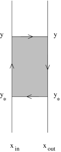
FIG. 4.: The eikonal solution to the magnetic scattering problem. The scattering amplitude (see Eq.(26)), is controlled by the flux encircled by the contour shown in the picture.

III Illustrations: Aharonov-Bohm scattering

To illustrate the usage of the paraxial theory, the scattering on the Aharonov-Bohm magnetic line is considered in this section as an example. Some results presented in this section has been published in a short communication Ref.[38].

The scattering problem is formulated as follows. The incident wave $\psi_{in}=\psi_{\text{in}}(y)$ comes from the negative side of the $x$-axis and the charge sees a magnetic line (extending in the $z$-direction), which creates the magnetic field $b(x,y)=\Phi_{0}\delta(x)\delta(y)$. The final goal is to characterize the outgoing wave at $x>0$.

As the magnetic field is finite only at the origin, the scattering region II in the terminology of Section II A can be shrunk to just the line $y=0$, so that $x_{in}=-0$ and $x_{out}=+0$. Seeing that scattering region is narrow, the eikonal approximation discussed in Section II B is applicable, except, perhaps, in the immediate vicinity of the singular magnetic line point $y=0$. The flux function, $\Phi(y)$, in the eikonal expression Eq.(26) is easily found to be $\Phi(y)=\Phi\theta(y)$ (if $y_{*}$ is chosen at $-\infty$) . The outcoming wave reads

$$\psi_{\text{out}}(y)=\exp\left(-i\pi\tilde{\Phi}sign(y)\right)\psi_{\text{in}}(y)\;.$$ (27)

where $\tilde{\Phi}\equiv{\Phi\over{\Phi_{0}}}$ [42]. Same result can readily obtained [38] by solving the first order differential equation Eq.(24) with the vector potential in the gauge

$\displaystyle A_{x}(x,y)=-{1\over 2}\Phi\,sign(y)\,\delta(x)\;\;,\;\;A_{y}(x,y)=0\;.$

The freely propagating outgoing wave is found from Eq.(22) with $x_{out}=0$ and $\psi_{\text{out}}$ from Eq.(27) Ref.[38],

$$\psi_{\text{out}}(x,y)=\psi_{\text{in}}(x,y)\cos{\pi\tilde{\Phi}}+iV(x,y)\sin{\pi\tilde{\Phi}}\;\;,\;\;x>0\ ,$$ (28)

where $\psi_{\text{in}}(x,y)$ is the incoming wave continued to the region $x>0$,

$$\psi_{\text{in}}(x,y)=\int\limits_{-\infty}^{\infty}dy^{\prime}G^{R}_{0}(x,y-y^{\prime})\psi_{\text{in}}(y^{\prime})\ ,$$ (29)

i.e. the wave in the absence of the Aharonov-Bohm line, and

$$V(x,y)=\int\limits_{-\infty}^{\infty}dy^{\prime}G^{R}_{0}(x,y-y^{\prime})\,\hat{y^{\prime}}\,\psi_{\text{in}}(y^{\prime})\ .$$ (30)

Eqs.(28 30) give the solution of the Aharonov-Bohm problem in the paraxial approximation for an arbitrary incoming wave $\psi_{in}(y)$.

Using Eq.(23), one can check that

$$\int\limits_{-\infty}^{\infty}dy\,|\psi_{\text{in}}(x,y)|^{2}=1\;\; \;\;\int\limits_{-\infty}^{\infty}dy\,|V(x,y)|^{2}=1\ ,$$ , (31)

$$\Im\int\limits_{-\infty}^{\infty}dy\;\psi^{*}_{\text{in}}(x,y ) V(x,y)=0;$$ (32)

for any $x>0$ and arbitrary (normalized) $\psi_{\text{in}}$; these relations guarantee the current conservation [43].

The solution in Eq.(28) gives a convenient tool for studying interaction of beams (waves packets) with the Aharonov-Bohm flux line. Some examples are considered below.

A Plane incident wave

Plane wave corresponds to $\psi_{\text{in}}(y)=1$. From Eqs.(29) and (23), one gets $\psi_{\text{in}}(x,y)=1$, and from Eq.(30) Ref.[38],

$$V(x,y)=K(\tilde{y})\;\;,\;\;\tilde{y}={y\over{\sqrt{2\lambdabar x}}}$$ (33)

where $K(t)$ is a familiar function,

$$K(t)={2\over{\sqrt{i\pi}}}\,\int\limits_{0}^{t}\,dt^{\prime}\,e^{it^{\prime 2}}\ ,$$ (34)

related to the Fresnel integrals. The outgoing wave Eq.(28) reads

$$\psi_{\text{out}}(x,y)=\cos{\pi\tilde{\Phi}}+iK(\tilde{y})\sin{\pi\tilde{\Phi}}\ .$$ (35)

The complex wave function $\psi_{\text{out}}(x,y)$ is a function of the real parameter $\tilde{y}$ only. This means, that $\psi_{out}(x,y)$ for any point of the half-plane $x>0$ spans a line on the complex plane $\Re\psi-\Im\psi$. This line (Fig. 5) is the Cornu spiral well-known in the diffraction theory [44]. The property of the Cornu spiral is that $(dt)^{2}$ is proportional to $(d\ell)^{2}$ where $d\ell$ is the distance between the points corresponding to $t$ and $t+dt$. From Eq.(33) and Eq.(34), the element $d\ell$ of the length along the spiral (the arc-length) and $d\tilde{y}$ are related as $(d\ell)^{2}={4\over\pi}\sin^{2}(\pi\tilde{\Phi})(d\tilde{y})^{2}$. Since the wave function Eq.(35) is real for $\tilde{y}=0$, the arc-length counted from the spiral point with $\Im\psi=0$ is proportional to $\tilde{y}$

FIG. 5.: The paraxial wave-function Eq.(35) on the $\psi$ -complex plane for the fluxes ${1\over 16}\Phi_{0}$, ${1\over 4}\Phi_{0}$, ${1\over 2}\Phi_{0}$, ${3\over 4}\Phi_{0}$, ${15\over 16}\Phi_{0}$. The points on the spirals are uniquely characterized by the spiral arc-length counted from the point where $Im\,\psi=0$ and measured in units proportional to $\sin\tilde{\Phi}$. For the point with the coordinates $x,y$, the wave function $\psi(x,y)$ corresponds to the point on the Cornu spiral with the arc-length equal to $\tilde{y}=y/\sqrt{2\lambdabar x}$ . In accordance with Ref.[45], the exact Aharonov-Bohm solution can be also mapped to the Cornu spiral; for a general scattering angle the mapping condition is that arc-length $\approx\sqrt{(r-x)/\lambdabar}$ in proper units.

The singular Aharonov-Bohm line problem gives a rather tough test for the validity of the paraxial approximation. The evaluation of its accuracy has been made simple by the recent observation Ref.[45] that the exact solution can be presented in the form Eq.(35) with $\tilde{y}\rightarrow\tilde{Y}$ with $\tilde{Y}$ found from

$$\tilde{Y}^{2}={(r-x)\over\lambdabar}+\varphi\left({1\over 2}-\tilde{\Phi}\right)+\ldots\;,$$ (36)

$r$ and $\varphi$ being the cylindrical coordinates; the terms not shown in Eq.(36) are of order ${\cal O}\left({\lambdabar\over r}\right)$ [45]. (Unexpectedly, the Aharonov-Bohm wave function on the $x-y$ plane can be mapped on the Cornu spiral not only in the forward direction but for any scattering angle (and $r\gg\lambdabar$), see Ref. [45] for details.) The paraxial approximation gives correctly the leading term $\sqrt{{r-x\over\lambdabar}}\approx\tilde{y}$ in the vicinity of the forward direction and short wave length $\lambdabar\ll r$.

B Finite size beam

The scattering of a plane wave by the Aharonov-Bohm line is highly singular: Eq.(35) shows that in the forward direction, $\varphi\ll\sqrt{{\lambdabar\over x}}$ i.e. $\tilde{y}\ll 1$, the wave function equals to $\cos\pi\tilde{\Phi}$ and does not converge at large distances to the plane incident wave as assumed in the standard scattering theory. Known from the exact solution [46], this anomaly is the reason why the text-book scattering theory fails: The incoming plane wave and scattered wave cannot be separated [46] and the scattering amplitude cannot be introduced as the object carrying the complete information about scattering [38].

The singular behaviour is due to the combination of two factors: (i) the infinitely long range of the interaction with the line; (ii) the infinite extension of the plane wave. Since any physical state has a finite transverse extension $W$, the behaviour of the potential beyond the width $W$ is irrelevant, and the singularities are expected to be regularized.

To show this, suppose that the incoming wave is beam-like with the profile

$\displaystyle\psi_{in}(y)=e^{-{y\over|W|}}\;,$where $W$ is the beam width; it is assumed that $W\gg\lambdabar$ so that the paraxial approximation is applicable. The beam has a small but finite angular width $\varphi_{0}=\lambdabar/W$. One can easily see from Eq.(28) that at large distances $x\gg W^{2}/\lambdabar$, the outgoing wave behaves like a spherical wave i.e. $|\psi_{out}(x,y)|^{2}\approx P(\varphi)/x$ where $\varphi=y/x$ is the scattering angle and $P(\varphi)$,

$$P(\varphi)={2\lambdabar\over\pi}{(\varphi\,\sin\pi\tilde{\Phi}-\varphi_{0}\cos\pi\tilde{\Phi})^{2}\over(\varphi^{2}+\varphi_{0}^{2})^{2}}\;,$$ (37)

has the meaning of the angular distribution of the intensity in the outgoing wave. As expected, the distribution shown in Fig. 6 is perfectly smooth.

FIG. 6.: Scattering of a beam by the Aharonov-Bohm line. The solid line shows the angular distribution of the intensity $P(\varphi)$ in Eq.(37) for the flux $\tilde{\Phi}=+1/4$ and the beam angular width $\varphi_{0}=0.1$. The dashed, line which is the Aharonov-Bohm cross-section Eq.(38) fits well the distribution at large enough angles $\gg\varphi_{0}$ where the intensity can be attributed to scattering. The central, $|\varphi|\lesssim\varphi_{0}$, peak has a nontrivial structure, asymmetric relative to $\varphi\rightarrow-\varphi$. The small angle left-right asymmetry, which is absent in the scattering cross-section, is responsible for the effective Lorentz force exerted by the Aharonov-Bohm line.

For the angles larger than the beam angular width, i.e. $|\varphi|\gg\varphi_{0}$, one gets from Eq.(37) that

$$P(\varphi)\approx{2\lambdabar\over\pi}\;{\sin^{2}\pi\tilde{\Phi}\over\varphi^{2}}\;,$$ (38)

recovering the small angle asymptotics of the Aharonov-Bohm scattering cross-section [34]

$$\left({d\sigma\over d\varphi}\right)_{\!\text{AB}}={\lambdabar\over 2\pi}\,{\sin^{2}\pi{\tilde{\Phi}}\over\sin^{2}{\phi\over 2}}\;.$$ (39)

It would be rather trivial if the angular broadening of the incident wave led just to a regularization of the forward scattering singularity. Most important is that a qualitatively new feature becomes seen: Unlike the Aharonov-Bohm cross-section Eq.(39) the angular distribution in Eq.(37) is left-right asymmetric. The antisymmetric part is concentrated in the forward direction $|\varphi|\lesssim\varphi_{0}$, i.e. within the angular width of the incoming wave i.e. in the region where the scattered and incident waves cannot be separated [47]. The asymmetry means that the beam is deflected by the Aharonov-Bohm line as a whole [38, 39]. The order of magnitude of the deflection is the initial angular width $\varphi_{0}\sim\lambdabar/W$. One may say that the Aharonov-Bohm line not only scatters the incident wave but also modifies the unscattered part of the wave. Later, it will be shown that in a system of many Aharonov-Bohm lines, the deflections by individual lines coherently add together, and the lines act as an effective magnetic field

The deflection of the beam $\Delta\varphi$ can be presented via the momentum $\Delta p_{\perp}={\hbar\over\lambdabar}\Delta\varphi$ transfered to the charge in the direction perpendicular to its initial velocity. A calculation details of which are collected in Appendix A gives the following result Ref.[38]:

$$\Delta p_{\perp}=\hbar|\psi_{\text{in}}(0)|^{2}\sin 2\pi{\Phi\over{\Phi_{0}}}$$ (40)

here the momentum transfer is expressed via the value of the normalized incoming wave at the position of the line. By comparison with the exact theory, the validity of this paraxial result has been confirmed by Berry [39].

IV Density matrix

The theory of magnetic scattering presented in Section II A is gauge invariant only in a limited sense. Although Eq.(20) holds in arbitrary gauge, each of the objects there, $\psi_{\text{in}}$, $\psi_{\text{out}}$, and ${\cal G}$ is gauge dependent, although only through the overall phase. For example, under $\mathchoice{{\hbox{\boldmath$\displaystyle A$}}}{{\hbox{\boldmath$\textstyle A$}}}{{\hbox{\boldmath$\scriptstyle A$}}}{{\hbox{\boldmath$\scriptscriptstyle A$}}}\rightarrow\mathchoice{{\hbox{\boldmath$\displaystyle A$}}}{{\hbox{\boldmath$\textstyle A$}}}{{\hbox{\boldmath$\scriptstyle A$}}}{{\hbox{\boldmath$\scriptscriptstyle A$}}}+\mathchoice{{\hbox{\boldmath$\displaystyle\nabla$}}}{{\hbox{\boldmath$\textstyle\nabla$}}}{{\hbox{\boldmath$\scriptstyle\nabla$}}}{{\hbox{\boldmath$\scriptscriptstyle\nabla$}}}\chi$ simultaneously with $\Psi\rightarrow e^{i{e\over{\hbar c}}\chi}$, the incoming wave $\psi_{\text{in}}$ Eq.(14) is modified as $\psi_{\text{in}}\rightarrow e^{i{e\over{\hbar}}\chi(\mathchoice{{\hbox{\boldmath$\displaystyle R$}}}{{\hbox{\boldmath$\textstyle R$}}}{{\hbox{\boldmath$\scriptstyle R$}}}{{\hbox{\boldmath$\scriptscriptstyle R$}}}_{I})}\psi_{\text{in}}$; we see also that the overall phase depends on the arbitrarily chosen $\mathchoice{{\hbox{\boldmath$\displaystyle R$}}}{{\hbox{\boldmath$\textstyle R$}}}{{\hbox{\boldmath$\scriptstyle R$}}}{{\hbox{\boldmath$\scriptscriptstyle R$}}}_{I}$. Of course, the observables are independent from the global phase and the above gauge dependence does not create any problem.

A truly gauge invariant theory can be formulated in terms of the by-linear in $\Psi$ and $\Psi^{*}$ “density matrix” $\rho(y_{1},y_{2};x)$ defined as

$$\rho(y_{1},y_{2};x)\equiv e^{-i{e\over{\hbar}}\int\limits_{y_{2}}^{y_{1}}dy^{\prime}\,A_{y}(x,y^{\prime})}\Psi(x,y_{1})\Psi^{*}(x,y_{2})\ .$$ (41)

The “density matrix” $\rho$ carries the full quantum information needed to find observables and is gauge invariant. In the field free regions, the density matrix is built from $\psi_{\text{in}}$ and $\psi_{\text{in}}^{*}$ or $\psi_{\text{out}}$ and $\psi_{\text{out}}^{*}$; these combinations depend on neither gauge nor $\mathchoice{{\hbox{\boldmath$\displaystyle R$}}}{{\hbox{\boldmath$\textstyle R$}}}{{\hbox{\boldmath$\scriptstyle R$}}}{{\hbox{\boldmath$\scriptscriptstyle R$}}}_{I,II}$.

The current density the $x$- and $y$- directions are (cf. Eq.(8))

$\displaystyle J_{x}(x,y)=v\rho(y,y;x)\;\;,\;\;J_{y}(x,y)={\hbar\over{2im}}\left({\partial\over{\partial y_{1}}}-{\partial\over{\partial y_{2}}}\right)\rho(y_{1},y_{2};x)\rule[-6.45831pt]{0.43057pt}{12.91663pt}_{y_{1}=y_{2}=y}$

Seeing that the evolution of the wave function $\Psi$ in Eq.(41) is given by the propagator $G^{R}$ Eq.(18), the density matrix evolves from $x^{\prime}$ to $x$ ($x>x^{\prime}$) as

$$\rho(y_{1},y_{2};x)=\int\limits_{-\infty}^{\infty}dy_{1}^{\prime}\,dy_{2}^{\prime}\,{\cal G}^{R}(y_{1},x;y_{1}^{\prime},x^{\prime})\,\rho(y_{1}^{\prime},y_{2}^{\prime};x^{\prime})\,{\cal G}^{A}(y_{2}^{\prime},x^{\prime};y_{2},x)$$ (42)

where ${\cal G}^{R}$ is defined by (21) and the advanced Green function ${\cal G}^{A}$

$\displaystyle{\cal G}^{A}(\mathchoice{{\hbox{\boldmath$\displaystyle r$}}}{{\hbox{\boldmath$\textstyle r$}}}{{\hbox{\boldmath$\scriptstyle r$}}}{{\hbox{\boldmath$\scriptscriptstyle r$}}}_{1},\mathchoice{{\hbox{\boldmath$\displaystyle r$}}}{{\hbox{\boldmath$\textstyle r$}}}{{\hbox{\boldmath$\scriptstyle r$}}}{{\hbox{\boldmath$\scriptscriptstyle r$}}}_{2})=\left({\cal G}^{R}(\mathchoice{{\hbox{\boldmath$\displaystyle r$}}}{{\hbox{\boldmath$\textstyle r$}}}{{\hbox{\boldmath$\scriptstyle r$}}}{{\hbox{\boldmath$\scriptscriptstyle r$}}}_{2},\mathchoice{{\hbox{\boldmath$\displaystyle r$}}}{{\hbox{\boldmath$\textstyle r$}}}{{\hbox{\boldmath$\scriptstyle r$}}}{{\hbox{\boldmath$\scriptscriptstyle r$}}}_{1})\right)^{*}\ .$

Introducing the two-particle Green function

$${\cal K}(y_{1},y_{2};x|y_{1}^{\prime},y_{2};,x^{\prime})={\cal G}^{R}(y_{1},x|y_{1}^{\prime},x^{\prime}){\cal G}^{A}(y_{2}^{\prime},x^{\prime}|y_{2},x)\ ,$$ (43)

Eq.(42) can be written as

$$\rho(y_{1},y_{2};x)=\int\limits_{-\infty}^{\infty}dy_{1}^{\prime}\,dy_{2}^{\prime}\,{\cal K}(y_{1},y_{2};x|y_{1}^{\prime},y_{2};,x^{\prime})\rho(y_{1}^{\prime},y_{2}^{\prime};x^{\prime})\,$$ (44)

As before, the incoming wave enters the scattering problem as the boundary condition at $x=x_{in}$: $\rho(y_{1},y_{2};x_{in})=\rho_{in}(y_{1},y_{2})$. Further propagation of the incoming beam is given by Eq.(44) with $x^{\prime}=x_{in}$.

For future references, we note the following property of the Green function:

$$\int\limits_{-\infty}^{\infty}dy\,G^{R}(x,y;x^{\prime},y_{1})\,G^{A}(x^{\prime},y_{2};x,y) = \theta(x-x^{\prime})\,\delta(y_{1}-y_{2})\ ,$$ (45)

$$\int\limits_{-\infty}^{\infty}dy\,G^{R}(x,y_{1};x^{\prime},y)\,G^{A}(x^{\prime},y;x,y_{2}) = \theta(x-x^{\prime})\,\delta(y_{1}-y_{2})\ ,$$ (46)

this relations expresses the current conservation [48].

In particular, from Eq.(45), one gets the conservation of the total current in the beam:

$\displaystyle\int dy\ \rho(y,y;x)=\int dy^{\prime}\rho(y^{\prime},y^{\prime};x=0)$

A Path integral representation

Similar to Eq.(7), the stationary paraxial equation in 2D may be mapped to a time dependent 1D problem:

$$i\hbar{\partial\over{\partial\tau}}\psi=\left(-{\hbar^{2}\over{2m}}\left({\partial\over{\partial y}}-i{e\over{\hbar c}}a\right)^{2}+e\varphi\right)\psi=0$$ (47)

where “time” $\tau={x\over{v}}$, $a=A_{y}$, and $\varphi=-{v\over{c}}A_{x}$. In the effective 1D problem, the particle moves in the “electric field”,

$$F=-{1\over{c}}\dot{a}-\nabla\varphi\ ,$$ (48)

defined by the “vector potential”, $a$, and the “scalar potential”, $\varphi$. The gauge transformation, $\mathchoice{{\hbox{\boldmath$\displaystyle A$}}}{{\hbox{\boldmath$\textstyle A$}}}{{\hbox{\boldmath$\scriptstyle A$}}}{{\hbox{\boldmath$\scriptscriptstyle A$}}}\rightarrow\mathchoice{{\hbox{\boldmath$\displaystyle A$}}}{{\hbox{\boldmath$\textstyle A$}}}{{\hbox{\boldmath$\scriptstyle A$}}}{{\hbox{\boldmath$\scriptscriptstyle A$}}}+\mathchoice{{\hbox{\boldmath$\displaystyle\nabla$}}}{{\hbox{\boldmath$\textstyle\nabla$}}}{{\hbox{\boldmath$\scriptstyle\nabla$}}}{{\hbox{\boldmath$\scriptscriptstyle\nabla$}}}\chi$, translates to $a\rightarrow a+\nabla\chi$, $\varphi\rightarrow\varphi-{1\over{c}}\dot{\chi}$, so that the effective electric field Eq.(48) is indeed gauge invariant. Locally, the electric field is related to the magnetic field of the original problem $b(x,y)$ as $F=-vb$.

The mapping to the effective 1D problem allows one to use a convenient path integral representation for the paraxial propagators. Obviously, $G^{R}$ is just the retarded Green function for nonstationary equation Eq.(47) and in the Feynman path integral representation

$\displaystyle G^{R}(x,y;x^{\prime},y^{\prime})=\int\limits_{y^{\prime}}^{y}{\cal D}[y(x)]e^{iS[y(x)]}$where the action of the effective 1D problem $S={1\over{\hbar}}\int d\tau(m\dot{y}^{2}/2+ea\dot{y}/c-e\varphi)$ translates as

$$S[y(x)]={1\over{2\lambdabar}}\int\limits_{x^{\prime}}^{x}dx\,y^{2}_{x}+{e\over{\hbar c}}\int\limits_{y=y(x)}\,d\mathchoice{{\hbox{\boldmath$\displaystyle r\cdot A$}}}{{\hbox{\boldmath$\textstyle r\cdot A$}}}{{\hbox{\boldmath$\scriptstyle r\cdot A$}}}{{\hbox{\boldmath$\scriptscriptstyle r\cdot A$}}}\ ,$$ (49)

where $y_{x}={dy\over{dx}}$. The action corresponding to ${\cal G}^{R}$ differs from Eq.(49) in the path of integration which should be extended in an obvious way to include the additional exponential factors in the definition of ${\cal G}^{R}$ Eq.(21).

With the help of Eq.(49), the two particle Green function Eq.(43) can be presented as

$${\cal K}(y_{1},y_{2};x|y_{1}^{\prime},y_{2};,x^{\prime})=\int{\cal D}[y_{1}(x)]{\cal D}[y_{2}(x)]e^{i{\cal S}[y_{1}(x),y_{2}(x)]}\ ,$$ (50)

where

$\displaystyle{\cal S}={\cal S}_{0}+{2\pi\over{\Phi_{0}}}\Phi([y_{1}],[y_{2}])\ ,$${\cal S}_{0}$ being the free motion contribution,

$${\cal S}_{0}[y_{1}(x),y_{2}(x)]={1\over{2\lambdabar}}\int\limits_{x^{\prime}}^{x}dx\,\left(y_{1x}^{2}-y_{2x}^{2}\right)\ ,$$ (51)

and $\Phi$ is the flux

$$\Phi([y_{1}],[y_{2}])=\oint\limits_{C([y_{1}],[y_{2}])}d\mathchoice{{\hbox{\boldmath$\displaystyle r\cdot A$}}}{{\hbox{\boldmath$\textstyle r\cdot A$}}}{{\hbox{\boldmath$\scriptstyle r\cdot A$}}}{{\hbox{\boldmath$\scriptscriptstyle r\cdot A$}}}$$ (52)

threading the (oriented) area bounded by the paths $y_{1}(x)$ and $y_{2}(x)$ and the vertical lines at $x$ and $x^{\prime}$ (see Fig.7).

FIG. 7.: The integration in Eq.(50) is performed with respect to the paths $y_{1}(x)$ and $y_{2}(x)$. Due to the phase factors introduced in Eqs.(14), and (19), the action contains the vector potential integrated along the closed loop shown here.

The path integral representation is used below to perform averaging with respect to the gauge field.

V Gaussian Random magnetic field

This Section concerns the averaging the two-particle Green’s function Eq.(43) with respect to the Gaussian random magnetic field Eq.(1). In the path integral representation Eq.(50), the random field enters via the flux $\Phi([y_{1}],[y_{2}])$ Eq.(52). For the Gaussian field Eq.(1), the averaged value

$\displaystyle\left<\exp\left(2\pi i{\Phi([y_{1}],[y_{2}])\over{\Phi_{0}}}\right)\right>=\exp\left(-{\cal A}_{\text{no}}([y_{1}-y_{2}])\over{2{\cal L}^{2}}\right)$where ${\cal A}_{\text{no}}$

$\displaystyle{\cal A}_{\text{no}}([y_{1}-y_{2}])=\int\limits_{x^{\prime}}^{x}dx\,|y_{1}-y_{2}|$is the non-oriented area bounded by the paths $y_{1}(x)$ and $y_{2}(x)$ and lines $x=x^{\prime}$ and $x=x$ (see Fig.7). Further calculations are rather simple thanks to the fact that $\left<e^{i2\pi{\Phi\over{\Phi_{0}}}}\right>$ is a functional only of $y_{1}-y_{2}$. This important simplification is a property of the models with a $\delta$-correlated magnetic field.

In the variables

$\displaystyle y=y_{1}-y_{2}\;\;,\;\;Y={1\over{2}}\left(y_{1}+y_{2}\right)\ ,$the kinetic energy contribution ${\cal S}_{0}$ Eq.(51) reads after integration by parts,

$\displaystyle{\cal S}_{0}[y_{1}(x),y_{2}(x)]={1\over{2\lambdabar}}y_{x}Y|_{x^{\prime}}^{x}-{1\over{2\lambdabar}}\int\limits_{x^{\prime}}^{x}dx\,y_{xx}Y\ .$Since $Y(x)$ enters only the ${\cal S}_{0}$, the integration $e^{i{\cal S}}$ with respect to $Y$ gives $\delta(y_{xx})$. This means, that the integration with respect to $y(x)$ is limited to the path with $y_{xx}\equiv{d^{2}y\over{dx^{2}}}=0$ that is the straight line connecting the initial and final points. After this, the integral is easily calculated.

Finally, ${\cal K}_{\text{av}}$ that is the paraxial two-particle Green function Eq.(43) averaged with respect to the fluctuation magnetic field, reads

$${\cal K}_{\text{av}}(y_{1},y_{2};x|y_{1}^{\prime},y_{2};,x^{\prime})={\cal K}_{\text{0}}(y_{1},y_{2};x|y_{1}^{\prime},y_{2};,x^{\prime})\exp\left(-{{\cal A}_{\text{no}}\over{{2\cal L}^{2}}}\right)\ ,$$ (53)

here ${\cal K}_{0}$ is the free two-particle propagator, and ${\cal A}$ is the (non-oriented) area formed by the straight line trajectories Fig.8,

FIG. 8.: The straight line trajectories contributing to the Feynman integral. ${\cal A}_{\text{no}}$ in Eq.(53) is the geometrical area inside the closed loop. If $(y_{1}-y_{2})(y_{1}^{\prime}-y_{2}^{\prime})<0$, the trajectories cross each other, and the area is built of two triangles.

$${\cal A} = {1\over 2}(x-x^{\prime})\times\left\{\begin{array}[]{lcr}|y_{1}+y_{1}^{\prime}-y_{2}-y_{2}^{\prime}|&,&\;\;\text{if }(y_{1}-y_{2})(y_{1}^{\prime}-y_{2}^{\prime})>0\rule[-12.91663pt]{0.0pt}{0.0pt}\\ {(y_{1}-y_{2})^{2}+(y_{1}^{\prime}-y_{2}^{\prime})^{2}\over{\mid y_{1}-y_{2}\mid+\mid y_{1}-y_{2}\mid}}&,&\text{if }(y_{1}-y_{2})(y_{1}^{\prime}-y_{2}^{\prime})<0\end{array}\right.$$ (56)

In the variables $y,Y$ and $(x-x^{\prime})\rightarrow x$, an expanded version of Eq.(53) reads

$$K_{\text{av}}(y,Y;y^{\prime},Y^{\prime};x) = {1\over{2\pi x\lambdabar}}\exp\Big{[}{i\over{x\lambdabar}}(Y-Y^{\prime})(y-y^{\prime})-{1\over{8}}{x\over{{\cal L}^{2}}}\Big{(}\mid y\mid+\mid y^{\prime}\mid+{(y+y^{\prime})^{2}\over{\mid y\mid}+\mid y^{\prime}\mid}\Big{)}\Big{]}$$ (57)

The two-particle Green function in Eq.(57) allows one to find averaged over the random field “evolution” of the density matrix and thus describes correlations in the gauge invariant observables like the density or the current. For instance, it describes transmission through a slab with a random magnetic field. In what follows, Eq.(57) is applied to some simple cases: (i) focusing of a coherent wave; (ii) the scattering of the partially coherent spatially uniform incoming wave.

A Coherent propagation: Focusing

Let the incident wave $\psi_{in}(y)$ be a converging Gaussian beam i.e.

$$\psi_{in}(y)={1\over{(\pi)^{1/4}\sqrt{w}}}e^{-{y^{2}\over{2}}({1\over{w^{2}}}+{i\over{\lambdabar f}})}\;,$$ (58)

where $f$ is the distance to the focal point and $w\ll f$ is the width of the beam. It is well-known that the “spherical” wave like that in Eq.(58) will converge at the focal point $x=f$ producing a diffraction limited spot with the waist $\sim\lambdabar/\theta$ where $\theta=w/f\ll 1$ is the angular size of the beam as seen from the focal point.

The distribution of the averaged intensity for the beam propagating in a random magnetic field can be found with the help of Eq.(57). Taking for simplicity only the points on the beam axis $y=0$, the intensity $I(x)\equiv\rho(0,0;x)$, reads

$\displaystyle I(x)={1\over{\sqrt{\pi}w}}{1\over{\lambda x}}\int\limits_{-\infty}^{\infty}\;dY\;dye^{i{1\over{\lambdabar}}\big{(}{1\over{x}}-{1\over{f}}\big{)}yY-{Y^{2}\over{w^{2}}}-{y^{2}\over{4w^{2}}}-{x\over{4{\cal L}^{2}}}\mid y\mid}\;.$At the focal point $x=f$,

$\displaystyle I(f)={1\over{\lambda f}}\int\limits_{-\infty}^{\infty}\;dye^{-{y^{2}\over{4w^{2}}}-{f\over{4{\cal L}^{2}}}\mid y\mid}\;,$In the limiting cases,

$$I(f)=\left\{\begin{array}[]{lcl}{2\sqrt{\pi}\over{\lambda f}}\times w&\;\;\;\;,&fw\ll{\cal L}^{2}\\ {8\over{\lambda f}}\times{{\cal L}^{2}\over{f}}&\;\;\;\;,&fw\gg{\cal L}^{2}\end{array}\right.\;.$$ (59)

For the conditions when the magnetic field is not important, the upper line gives the usual diffraction limited value of the intensity; the width of the spot at the focal plane (line) is of order of $\sim 1/I(f)\sim\lambdabar/\theta$, where $\theta=w/f$. The larger the aperture $w$, the larger the intensity in the focus and the smaller the size of the spot. However, in the presence of the random magnetic field, the intensity saturates when the aperture $w\sim{\cal L}^{2}/f$ and $\theta\sim\left({\cal L}/f\right)^{2}$.

This behaviour is very different from that when the scattering is due to a random scalar potential with a short correlation length. In this case, the relevant parameter characterizing the disorder is the focal length $f$ in units of the mean free path $l$ rather then the size of the aperture: On the background created by incoherent scattering, one would see a spot with the disorder insensitive profile and the integral intensity $\propto e^{-f/l}$ (the exponential factor is probability that the wave does not experience any scattering).

B Incoherent wave: the Boltzmann equation

Consider the initial density matrix of the form $\rho_{in}(y_{1},y_{2})=\rho_{0}(y_{1}-y_{2})$, $y=y_{1}-y_{2}$, which corresponds to a partially coherent spatially homogeneous state. At $x>0$, the density matrix $\rho(y_{1},y_{2};x)=\rho(y;x)$ is found from Eq.(44) with the two-particle propagator from Eq.(57). The Fourier transform,

$$\rho(y;x)=\int\limits_{-\infty}^{\infty}d\varphi\,e^{i\varphi{y\over{\lambdabar}}}\,n_{\varphi}(x)\ ,$$ (60)

defines $n_{\varphi}$ which has the meaning of the distribution function with respect of the transverse momentum, $q=\varphi{\hbar\over{\lambdabar}}$, and $\varphi$ is the angle between the velocity of the particle and the $x$-axis. In the paraxial situation, the distribution is concentrated at small angles and the integration in Eq.(60) can be taken in infinite limits.

From, Eqs.(44) and (57) we easily get the density matrix of the wave having traveled the distance $x$:

$$\rho(y;x)=\rho_{0}(y)\exp\left({-{x\mid y\mid\over{2{\cal L}^{2}}}}\right)\ .$$ (61)

As required by the current conservation, $\rho(0;x)$ does not depend on $x$ whereas the non-diagonal elements of the density matrix $y\neq 0$ decay to zero, the faster, the more “distance to the diagonal” $|y|$. In other words, random magnetic field is very effective in destroying a long range coherence, the longer the coherence, the faster it decays.

Considering the limiting case of plane infinite incident wave $n_{\varphi}(x=0)=\delta(\varphi)$ i.e. $\rho_{in}(y)=1$, Eq.(61) gives

$$n_{\varphi}(x)={1\over\pi}{\Delta\over\varphi^{2}+\Delta^{2}}\;\;,\;\;\Delta=x{\lambdabar\over 2{\cal L}^{2}}$$ (62)

The evolution is nonperturbative in the sense that the plane wave looses its shape immediately at any $x\neq 0$ transforming into the Lorentz distribution with the width of the distribution proportional to $x$ and the strength of the field [49]. In particular, it means that the plane wave is not a good basis for the perturbation theory.

More insight can be gained if the evolution of the density matrix is mapped to a Boltzmann-type kinetic equation. For this, note that the density matrix in Eq.(61) satisfies the equation,

$$v{\partial\over{\partial x}}\rho+\hat{I}\rho=0\;\;,\;\;\hat{I}={v\over 2{\cal L}^{2}}|y|\ .$$ (63)

Written for the distribution function $n_{\varphi}$ introduced in Eq.(60), the equation acquires the familiar Boltzmann form,

$$v{\partial n_{\varphi}\over{\partial x}}+\hat{I}n_{\varphi}=0\ ,$$ (64)

where $\hat{I}$ is the collision integral i.e. operator $\hat{I}$ in the $\varphi$-representation.

One may present the collision integral in the standard form

$$\hat{I}n_{\varphi}=\int d\phi\;w(\phi)(n_{\varphi}-n_{\varphi+\phi})\;\;,$$ (65)

where $w(\phi)$ is the scattering rate for the process $\varphi\rightarrow\varphi+\phi$. From the condition that the operators in Eq.(64) and Eq.(65) have same eigenvalues corresponding to the common eigenfunctions, $n_{\varphi}\sim e^{i{y_{0}\over\lambdabar}\varphi}$, $w$ must satisfy the requirement that Ref.[50]

$$\int\limits_{-\infty}^{\infty}d\phi\,w(\phi)(1-e^{-i{y_{0}\over{\lambdabar}}\phi})={v\over 2{\cal L}^{2}}|y_{0}|\ .$$ (66)

From here,

$$w(\phi)={2\over{\pi\tau_{0}}}{1\over{\phi^{2}}}\;\;,\;\;{1\over\tau_{0}}={v\lambdabar\over 4{\cal L}^{2}}$$ (67)

Usually, one can split the collision integral into the in- and out-scattering pieces. In the case of random magnetic field, the scattering-out rate is ill-defined as $\int d\phi w(\phi)$ diverges at small angles, and the split hardly makes sense. On the other hand, the collision integral, as an operator acting on the distribution function, is well defined and the transport is not singular.

Treating the random magnetic field in the Born approximation, Aronov et al. [14] found the the scattering rate $W(\phi)$ to be

$$W(\phi)={1\over{2\pi\tau_{0}}}\cot^{2}{{\phi\over 2}}\ .$$ (68)

Because of divergence at small angles, one may doubt the validity of the Born approximation. However, the small $\phi$ asymptotics of $W(\phi)$ agrees with Eq.(67). This means that Eq.(68) is actually valid for arbitrary $\phi$ if used for constructing the collision integral. The other way around, the collision integral Eq.(65) is expected to correctly describe scattering with arbitrary scattering angles if $W(\phi)$ Eq.(68) is used instead of paraxial $w(\phi)$ in Eq.(67). This allows one to generalize the paraxial kinetic equation, including large angle scattering.

The kinetic equation for the distribution function $n_{\varphi}$ reads

$$\mathchoice{{\hbox{\boldmath$\displaystyle v\cdot\nabla$}}}{{\hbox{\boldmath$\textstyle v\cdot\nabla$}}}{{\hbox{\boldmath$\scriptstyle v\cdot\nabla$}}}{{\hbox{\boldmath$\scriptscriptstyle v\cdot\nabla$}}}n_{\varphi}+\hat{I}n_{\varphi}=0\;\;,\;\;0<\varphi<2\pi\ ,$$ (69)

where the collision integral

$\displaystyle\hat{I}n_{\varphi}={1\over\tau_{0}}\int\limits_{0}^{2\pi}{d\phi\over 2\pi}\,\cot^{2}{{\phi\over 2}}\,\left(n_{\varphi}-n_{\varphi+\phi}\right)\ .$As before, the spilt of the collision integral in the in- and out- scattering parts leads to divergences and, therefore, has a very limited sense. At the same time, the collision operator is well-defined: If $n_{\varphi}$ is presented as the sum,

$\displaystyle n_{\varphi}=\sum\limits_{m}n_{m}e^{im\varphi}\ ,$over the eigenfunctions of the collision operator $e^{im\varphi}$, $m=0,\pm 1,\ldots$, the collision operator acts as

$\displaystyle\hat{I}n_{\varphi}={1\over\tau_{0}}\sum\limits_{m\neq 0}^{\infty}(2|m|-1)n_{m}e^{im\varphi}\;,$The parameter $\tau_{0}$ has the meaning of the relaxation time for the first harmonics $m=\pm 1$ i.e. the transport relaxation time.

One concludes that transport of a charge in a random magnetic field can be described by the Boltzmann equation, and is not anomalous in spite of the fact that the total scattering rate is infinite.

VI Random array of Aharonov-Bohm lines

This section deals with the model of a random gauge field where the gauge field is created by an array of Aharonov-Bohm lines. It is assumed that the lines in the array take random space positions and the flux of a line $\Phi$ may be random. The model is specified by the averaged density of the lines $d_{{}_{\text{AB}}}$ and the probability distribution $p(\Phi)$ for the magnetic flux $\Phi$ in a line. Our primarily goal is to average the paraxial two-particle Green function Eq.(43) over the distribution of the lines.

The calculations turn out to be very similar to those in Section V so that we only outline them. Repeating the arguments from Section V one comes to an expression similar to Eq.(53):

$\displaystyle{\cal K}_{\text{av}}(y_{1},y_{2};x|y_{1}^{\prime},y_{2};,x^{\prime})={\cal K}_{\text{0}}(y_{1},y_{2};x|y_{1}^{\prime},y_{2};,x^{\prime})\left<\exp\left(2\pi i{\Phi^{(t)}(y_{1},y_{2};x|y_{1}^{\prime},y_{2};,x^{\prime})\over{\Phi_{0}}}\right)\right>$where $\Phi^{(t)}(y_{1},y_{2};x|y_{1}^{\prime},y_{2};,x^{\prime})$ is the flux through the oriented area bounded by the straight (directed) lines connecting the initial and finite points (see Fig.8). Given the configuration of the Aharonov-Bohm array, the flux through the area is the sum over the lines piercing the area. The $k$’s line with the flux $\Phi_{k}$ contributes to the total flux as $\sigma_{k}\Phi_{k}$ where $\sigma_{k}=+1$ or $-1$ depending on the orientation, positive or negative, of the area the line is situated in. Let $N_{+}$ ($N_{-}$) be the (random) number of lines in the area with positive (negative) orientation; The variables $\Phi_{k}$’s are independent in the model, and the averaging $\exp\big{(}2\pi i{\Phi^{(t)}\over\Phi_{0}}\big{)}$ over the configurations with fixed $N_{\pm}$ is simple:

$\displaystyle\left<\exp\left(i{2\pi\over\Phi_{0}}\sum\limits_{k=1}^{N_{+}+N_{-}}\sigma_{k}\Phi_{k}\right)\right>=\left<\exp\left(2\pi i{\Phi\over\Phi_{0}}\right)\right>^{N_{+}}\left<\exp\left(-2\pi i{\Phi\over\Phi_{0}}\right)\right>^{N_{-}}$where $<\exp({\pm{2\pi i\Phi\over\Phi_{0}}})>$ implies averaging with the distribution function $p(\Phi)$.

The random numbers $N_{\pm}$ obey the Poisson distribution $P_{N}=e^{\bar{N}}\bar{N}^{N}/N!$ with $\bar{N}$ either $\overline{(N_{+}+N_{-})}=d_{{}_{\text{AB}}}{\cal A}_{\text{no}}$ or $\overline{N_{+}-N_{-}}=d_{{}_{\text{AB}}}{\cal A}_{\text{o}}$, ${\cal A}_{\text{no}}$ and ${\cal A}_{\text{o}}$ being non-oriented and oriented area, respectively.

Finally,

$\displaystyle\left<\exp\left(2\pi i{\Phi(y_{1},y_{2};x|y_{1}^{\prime},y_{2};,x^{\prime})\over{\Phi_{0}}}\right)\right>=\exp\left(-{{\cal A}_{\text{no}}\over{2\cal L}_{AB}^{2}}+i{2\pi\over\Phi_{0}}\tilde{B}{\cal A}_{\text{o}}\right)\ ,$where ${\cal A}_{\text{no}}$ is the non-oriented area Eq.(56), ${\cal A}_{\text{o}}$ is the oriented area,

$\displaystyle{\cal A}_{\text{o}}=-{1\over{2}}(x-x^{\prime})(y_{1}+y_{1}^{\prime}-y_{2}-y_{2}^{\prime})\ ,$

$${1\over{\cal L}_{AB}^{2}}=2d_{{}_{\text{AB}}}\left<1-\cos 2\pi{\Phi\over\Phi_{0}}\right>$$ (70)

and the effective magnetic field

$$\tilde{B}=d_{{}_{\text{AB}}}{\Phi_{0}\over 2\pi}\left<\sin 2\pi{\Phi\over\Phi_{0}}\right>\ ;$$ (71)

in Eqs.(70) and (71), the averaging is performed with the distribution function of the flux in the line $p(\Phi)$.

Collecting the results together, the two-particle Green function reads

$$K_{\text{av}}(y,Y;y^{\prime},Y^{\prime};x) =$$ (73)

$$={1\over{2\pi x\lambdabar}}\exp\left[{i\over{x\lambdabar}}(Y-Y^{\prime})(y-y^{\prime})-{1\over{8}}{x\over{{\cal L}_{{}_{\text{AB}}}^{2}}}\Big{(}\mid y\mid+\mid y^{\prime}\mid+{(y+y^{\prime})^{2}\over{\mid y\mid}+\mid y^{\prime}\mid}\Big{)}-i{\pi\over\Phi_{0}}\,\tilde{B}\,x(y+y^{\prime})\right]$$

where $y=y_{1}-y_{2}$, $y^{\prime}=y_{1}^{\prime}-y_{2}^{\prime}$, $Y={1\over{2}}(y_{1}+y_{2})$ $Y^{\prime}={1\over{2}}(y_{1}^{\prime}+y_{2}^{\prime})$ and $x\leftarrow(x-x^{\prime})$.

If compared with the Green function derived in Sect.V Eq.(57), the propagator Eq.(73) contains an additional term proportional $\tilde{B}$, finite to the extent the distribution $p(\Phi)$ is asymmetric. As we will see later, $\tilde{B}$ creates the Lorentz force and plays in dynamics the role of an effective magnetic field. A finite Lorentz force in an Aharonov-Bohm array is not readily obvious: A classical Lorentz force is absent since magnetic field is locally zero, whereas the quantum Aharonov-Bohm cross-section Eq.(39) is left-right and $\Phi\rightarrow-\Phi$ symmetric and cannot explain $\tilde{B}$. Obviously, $\tilde{B}$ and the associated force is directly related to the transverse momentum transfer considered in Sect.III (see Eq.(A3)).

In the limit of dense array with small typical flux, $\Phi\rightarrow 0$, $d_{{}_{\text{AB}}}\rightarrow\infty$, the effective field $\tilde{B}$ reduces to to the macroscopic mean-field magnetic induction $B=d_{{}_{\text{AB}}}<\Phi>$. In this limit, the Aharonov-Bohm array model is equivalent the $\delta-$correlated field model Eq.(1) with ${\cal L}^{-2}\propto d_{{}_{\text{AB}}}<\Phi^{2}>$, in the external homogeneous magnetic field $\tilde{B}$.

In general, however, $\Phi$-periodic $\tilde{B}$ Eq.(71) is very different from the mean-field expectations. Depending on the flux distribution function $p(\Phi)$, the magnetic induction and $\tilde{B}$ may be in any relation. For instance, the mean-field induction can be always compensated to zero by adding some properly oriented lines of flux $\Phi_{N}={N\over 2}\Phi_{0},\,N=1,2,\ldots$. However, the added lines do not affect the effective magnetic field $\tilde{B}$ seen by the particles (since $\sin\left(2\pi{\Phi_{N}\over\Phi_{0}}\right)=0$). In an Aharonov-Bohm array the Lorentz force may be finite even when the macroscopic magnetic induction is zero.

A Kinetic equation

As before, in Sect.V B, consider the spatially uniform situation when the density matrix of the partially coherent wave at $x=0$ is of the form $\rho_{in}(y_{1},y_{2})=\rho_{0}(y)$, $y=y_{1}-y_{2}$. The density matrix $\rho(y;x)$ of the wave at distance $x$ can be found from Eqs.(44) and Eq.(73),

$\displaystyle\rho(y;x)=\rho_{0}(y)\exp\left({-{x\mid y\mid\over{2{\cal L}_{AB}^{2}}}}-i{2\pi\over\Phi_{0}}\,\tilde{B}\,xy\right)\ .$Again, as in Sect.V B, the density matrix obeys the following kinetic equation (compare with Eq.(63)):

$\displaystyle v{\partial\over{\partial x}}\rho+i{2\pi\over\Phi_{0}}\tilde{B}y\rho+\hat{I}_{{}_{AB}}\rho=0\;\;,\;\;\hat{I}_{{}_{AB}}={v\over 2{\cal L}_{AB}^{2}}|y|.$Performing the Fourier transform, one gets the equation for the distribution function $n_{\varphi}$ in Eq.(60):

$$v{\partial n_{\varphi}\over{\partial x}}+{e\tilde{B}\over mc}{\partial n_{\varphi}\over{\partial\varphi}}+\hat{I}_{{}_{AB}}n_{\varphi}=0\ .$$ (74)

The equation has the Boltzmann form and $\tilde{B}$ enters kinetics as a magnetic field. The collision integral $\hat{I}_{{}_{AB}}$ has the form of Eq.(65) with the scattering rate

$\displaystyle W(\phi)={v\lambdabar\over 2\pi{\cal L}^{2}_{{}_{AB}}}{1\over{\phi^{2}}}$From here one can conclude that the relaxation is governed by an incoherent scattering by the flux lines: Indeed, $W$ is proportional to the density of lines and the contribution of a line is given by the small limit of the Aharonov-Bohm cross-section Eq.(39). Since even most dangerous small angle scattering fits this simple picture, it seems plausible that Eq.(74) can be generalized to arbitrary scattering angle using Eq.(39) as the probability scattering. Similar to Eq.(69), the kinetic equation reads

$\displaystyle\mathchoice{{\hbox{\boldmath$\displaystyle v\cdot\nabla$}}}{{\hbox{\boldmath$\textstyle v\cdot\nabla$}}}{{\hbox{\boldmath$\scriptstyle v\cdot\nabla$}}}{{\hbox{\boldmath$\scriptscriptstyle v\cdot\nabla$}}}n_{\varphi}-{e\tilde{B}\over mc}{\partial n_{\varphi}\over{\partial\varphi}}+\hat{I}_{{}_{AB}}n_{\varphi}=0\;\;,\;\;0<\varphi<2\pi\ ,$where the collision integral

$\displaystyle\hat{I}_{{}_{AB}}n_{\varphi}={1\over 2\tau_{{}_{AB}}}\int\limits_{0}^{2\pi}{d\phi\over 2\pi}\,{1\over\sin^{2}{{\phi\over 2}}}\,\left(n_{\varphi}-n_{\varphi+\phi}\right)\ .$with

$${1\over\tau_{{}_{AB}}}={\hbar\over m}d_{{}_{\text{AB}}}\left<1-\cos 2\pi{\Phi\over\Phi_{0}}\right>\ .$$ (75)

As before, the collision integral is a regular linear operator regardless its singular scattering-out term. Its action is defined by the following relation

$\displaystyle\hat{I}_{{}_{AB}}e^{im\varphi}={|m|\over\tau_{{}_{AB}}}\,\,e^{im\varphi}$From here, one sees that $\tau_{{}_{AB}}$ has the meaning of the transport scattering time.

Applicability of the Boltzmann equation requires the mean free path $l\sim v\tau_{{}_{AB}}$ to be large on the scale of the wave length $\lambdabar$.

$${\lambdabar\over l}\sim\lambdabar^{2}d_{{}_{\text{AB}}}\left<\sin^{2}{\pi{\Phi\over\Phi_{0}}}\right>\ll 1$$ (76)

If typically $\Phi/\Phi_{0}\sim 1$, the density of the lines must not be too high: $d_{{}_{\text{AB}}}\lambdabar^{2}\ll 1$. In case of lines with small $\Phi$, the condition is milder: $\Phi^{2}d_{{}_{\text{AB}}}\lambdabar^{2}\ll 1$.

As an illustration, the Drude conductivity tensor can be readily derived from the Boltzmann equation Eq.(75):

$$\sigma_{xx} = {1\over{2}}\,e^{2}\,N_{0}\,v^{2}\tau_{{}_{AB}}{1\over 1+(\Omega_{c}\tau_{{}_{AB}})^{2}}$$ (77)

$$\sigma_{xy} = (\Omega_{c}\tau_{{}_{AB}})\sigma_{xx}$$ (78)

where $N_{0}$ is the density of states and $\Omega_{c}={e\tilde{B}\over mc}$ plays the role of the Larmor frequency. One sees that the Hall angle $\theta_{H}$, $\tan\theta_{H}=\sigma_{xy}/\sigma_{xx}$,

$$\tan\theta_{H}={\left<\sin 2\pi{\Phi\over\Phi_{0}}\right>\over\left<1-\cos 2\pi{\Phi\over\Phi_{0}}\right>}\ ,$$ (79)

does not depend on the density of lines and parameters of the system. If the Aharonov-Bohm lines in array have same flux $\Phi$, the Hall angle is simply

$$\tan\theta_{H}=\cot\left(\pi{\Phi\over\Phi_{0}}\right)\ .$$ (80)

Counter intuition, the Hall effect is strongest at $\Phi\rightarrow 0$.

B Landau quantization

The Hall angle Eq.(80) in an Aharonov-Bohm array may be large which means that the particle orbit tends to be a circle, similar to Larmor orbits in an external magnetic field. The periodic classical motion is expected to be quantized (the Landau quantization). To check this possibility, one should calculate the density of states of a particle moving in an Aharonov-Bohm array. In the quasiclassical region, when the energy of the particle $E\gg\hbar\Omega_{c}$, the problem can be generally solved by the method used in [15]. In the present paper, only the most promising case of small flux array is considered. Not to repeat the calculation in [15], qualitative arguments which lead to the same result, are presented.

In the linear in $\Phi$ approximation, when scattering $\propto\Phi^{2}$ can be neglected, the transverse momentum Eq.(40) is transfered to the particle, and it undergoes periodic motion with the angular frequency $\Omega_{c}={e\tilde{B}\over mc}$ along the Larmor circle with the radius $R_{L}=v/\Omega_{c}$. In the small $\Phi$-limit, the distinction between $\tilde{B}$ and magnetic induction is immaterial, and the Bohr-Sommerfeld quantization condition can be formulated as the requirement of the flux quantization,

$$\Phi^{\text{orbit}}(E_{N})=\Phi_{0}(N+{1\over{2}})\ ,$$ (81)

where $\Phi^{\text{orbit}}(E)$ is the total flux encircled by an orbit of the particle with energy $E$. Due to the randomness in the flux line positions, the number of the encircled lines fluctuates, and so does the total flux. The total flux $\Phi^{\text{orbit}}=\langle\Phi^{\text{orbit}}\rangle+\delta\Phi$ is a random Gaussian variable which fluctuates around the average $\langle\Phi^{\text{orbit}}\rangle=\tilde{B}S(E)$, $S(E)=\pi R_{L}^{2}$ being the Larmor circle area. For the flux lines with uncorrelated positions, the total flux fluctuates with the variance

$$\langle\big{(}\delta\Phi\big{)}^{2}\rangle=d_{{}_{\text{AB}}}S(E)\langle\Phi^{2}\rangle\ .$$ (82)

Driven by the flux enclosed by the orbit, the energy of the level fluctuates, $E_{N}=\langle E_{N}\rangle+\delta E$. Neglecting the flux fluctuations in Eq.(81), $\Phi^{\text{orbit}}\rightarrow\langle\Phi^{\text{orbit}}\rangle$, one gets the average energy of the N-th level $\langle E_{N}\rangle=\hbar\Omega_{c}(N+{1\over{2}})$. To preserve the quantization Eq.(81), the level energy acquires a shift $\delta E$ under the flux variations $\delta\Phi$: From the condition

$\displaystyle\delta\Phi+\delta E_{N}{\partial\Phi\over{\partial E}}|_{E_{N}}=0\;,$one gets the energy shift caused by the change of the flux $\delta\Phi$:

$$\delta E_{N}=-\hbar\Omega_{c}{\delta\Phi\over\Phi_{0}}\ .$$ (83)

Combining Eq.(83) and Eq.(82), we see that the Landau levels acquire the Gaussian distribution form with variance (the width of the level)

$$\left<\big{(}\delta E_{N}\big{)}^{2}\right>={1\over\pi}\,{\hbar\over\tau_{{}_{AB}}}\,E$$ (84)

Physics here is similar to the inhomogeneous broadening: The Larmor circle sees different realizations of the random relief in different places of the “sample”, and the energy levels adjust their positions to the local conditions.

As already noticed in [15], it is rather unusual that importance of disorder (measured by the Landau level broadening Eq.(84)) increases with the energy $E$. The physical reason for this is that the larger is proportional to $E$ the area under the Larmor circle, the bigger are the absolute fluctuations of the number of the Aharonov-Bohm lines encircled by the orbit and the flux fluctuation $\delta\Phi$.

The density of states is given by the sum over the discrete levels. The position of the level is the Gaussian of the width in Eq.(84) and centered at $E_{N}=\hbar\Omega_{c}(N+{1\over{2}})$. The overlapping Landau levels create oscillating density of states. Similar to Ref.[15], one applies the Poisson summation formula and finds the first harmonics of the oscillations:

$\displaystyle\rho^{osc}(E)=-{m\over\pi\hbar^{2}}\exp(-\gamma)\cos\left(2\pi{E\over\hbar\Omega_{c}}\right)\;\;,$where the damping of the oscillations is controlled by

$\displaystyle\gamma={2\pi\over\Omega_{c}\tau_{{}_{AB}}}\,{E\over\hbar\Omega_{c}}\ .$Therefore, the Shubnikov-De-Haas oscillations in the Aharonov-Bohm array are strongly suppressed: even when $\Omega_{c}\tau_{{}_{AB}}=\tan\theta_{H}\gtrsim 1$ and the Larmor circling is well pronounced, quasiclassical quantization at high Landau levels $E\gg\hbar\Omega_{c}$ may not be seen because of the large damping $\gamma$.

The damping parameter $\gamma$ can be also presented as

$$\gamma={\pi\over 2}\,{1\over\lambdabar^{2}d_{{}_{\text{AB}}}}\,{\langle\Phi^{2}\rangle\over\langle\Phi\rangle^{2}}\,\,\,\geq\,\,\,{\pi\over 2}{1\over\lambdabar^{2}d_{{}_{\text{AB}}}}$$ (85)

where $\lambdabar$ ($=\hbar/\sqrt{2mE}$) is the wave length corresponding to the energy $E$; the equality sign realizes in the case when the lines have equal flux. One concludes from Eq.(85) that as a necessary condition, the Larmor motion may be quantized only if the wave length exceed the distance between Aharonov-Bohm lines. As one could expect, this requirement tends to be complementary to the condition of applicability of the Boltzmann equation in Eq.(76).

VII Conclusions

The main goal of the paper has been to understand specific features of the transport properties of a quantum charge subject to a random magnetic field, namely, the features related to the long range correlations of the gauge potential and the anomalous forward scattering. The non-perturbative method used in the paper to handle the divergence is based on the paraxial approximation to the stationary Schrödinger equation (Section II).

The paraxial theory of magnetic scattering is presented in Section II A. To show usage of the theory, it is applied to the Aharonov-Bohm line problem in Section III. Being calculationally simple, the paraxial approximation proves to be rather efficient. The paraxial solution reproduces the small angle asymptotics of the Aharonov-Bohm exact solution for the plane incident wave. The wave packet solution (see Eq.(37)) allows one to resolve an old controversy discussed in the Introduction concerning the transverse force exerted by the Aharonov-Bohm line. One sees that the angular distribution in the outgoing wave is indeed left-right asymmetric, so that there is a finite momentum transfer in the transverse direction. However, the asymmetry is concentrated within the angular width of the incident wave and it cannot be described in terms of the differential cross-section. For an arbitrary incident wave, the transverse momentum transfered to the charge can be found by Eq.(40). By comparison with the exact solution, the validity of this formula has been recently confirmed by Berry [39].

The main result of the paper is the paraxial two-particle Green’s function averaged with respect to the random magnetic field. In the paraxial theory, a stationary 2D problem becomes equivalent to a non-stationary 1D one, and one can use the standard Feynman representation for the propagators. It turns out that the corresponding path integral can be evaluated exactly. The expressions for the Green’s function is given by Eqs.(57) and Eq.(73) for the Gaussian random magnetic field and the Aharonov-Bohm array model, respectively.

The paraxial two-particle Green’s function solves the quantum problem of the near forward multiple scattering by random gauge potential: for a given incident wave, one is able to find correlators $\langle\psi(\mathchoice{{\hbox{\boldmath$\displaystyle r$}}}{{\hbox{\boldmath$\textstyle r$}}}{{\hbox{\boldmath$\scriptstyle r$}}}{{\hbox{\boldmath$\scriptscriptstyle r$}}}_{1})\psi^{*}(\mathchoice{{\hbox{\boldmath$\displaystyle r$}}}{{\hbox{\boldmath$\textstyle r$}}}{{\hbox{\boldmath$\scriptstyle r$}}}{{\hbox{\boldmath$\scriptscriptstyle r$}}}_{2})\rangle$, where averaging is performed with respect to the random field. To draw physical conclusions, two cases are analyzed: (i) (de)focusing of a coherent converging wave in the random magnetic field environment, and (ii) propagation of spatially homogeneous partially coherent beam.

The non-local character of interaction with magnetic field is clearly seen from the analysis in Section V A of defocusing of a converging beam. The lost of coherence measured by defocusing is controlled by the size of the entire area “occupied “ by the system that is the region where the wave function is finite: Indeed, it follows from Eq.(59) that the wave cannot be focussed if the random flux threading the area (aperture size)$\times$(focus length) is of order of the flux quantum $\Phi_{0}$. Same conclusion follows from Eq.(62): having traveled a distance $x$, a perfect plane wave becomes a mixture of waves with the transverse momenta $\Delta p_{y}\sim\hbar x/{\cal L}^{2}$ where the spatial coherence survives only within the region $\Delta y\sim{\cal L}^{2}/x$. Again, supporting the qualitative arguments presented in the Introduction, the coherence exists only within the area $\Delta x\times\Delta y\sim{\cal L}^{2}$; the area is defined by the condition that the random flux is typically not bigger than the flux quantum $\Phi_{0}$.

On the other hand, the evolution in the momentum space is rather ordinary: It is described by the usual Boltzmann equation derived in Sections V B and VI A. The only uncommon feature of the Boltzmann equation is that the collision integral being a well-defined operator nevertheless cannot be split in the scattering -in and -out regular parts: An attempt of the split produces two singular pieces, the two infinities canceling when combined. In the diagrammatic language, this can be rephrased as the cancellation of the divergences in the self energy and the vertex correction as observed in Ref.[25].

The condition of applicability of the paraxial approximation can be derived from Eq.(12): At the distance $x$, the typical transverse size $w$ is of order $min\,[w_{0},{\cal L}^{2}/x]$ where $w_{0}$ is the characteristic length in the initial distribution. For large enough $x$, $w\sim{\cal L}^{2}/x$. Substituting this value into Eq.(12), one gets

$\displaystyle x<x_{max}\;\;,\;\;x_{max}\equiv{\cal L}\left({{\cal L}\over\lambdabar}\right)^{{3\over 5}}\;.$One sees that the theory is applicable in the non-perturbative region $x\gg{\cal L}$ in the paraxial limit $\lambdabar\ll{\cal L}$.

In the paraxial picture, the particle always moves in (almost) same direction. Therefore, any effect related to the Anderson localization is beyond the paraxial approximation. Although the Boltzmann equation allows for large angle scattering events, it is, of course, unable to describe the quantum localization either. Localization in random magnetic field remains a controversial issue, see Refs.[14] and [20].

Two models of the random field has been considered in the paper: the Gaussian random magnetic field with zero average and the array of Aharonov-Bohm magnetic flux lines with arbitrary distribution of the line fluxes. Comparing the Green’s function in Eqs.(57), and (73) (with $\tilde{B}\rightarrow 0$), one sees that the models are paraxially equivalent. (For the Gaussian model, Eq.(57) has been derived assuming that the field is zero on average, $\langle b\rangle=0$. In a more general case, the Gaussian model with a finite magnetic induction $B=\langle b\rangle$ has the Green’s function of the form in Eq.(73) with $\tilde{B}$ substituted for $B$).

The origin of the effective magnetic field in the Aharonov-Bohm array can be traced back to the left-right asymmetry in the scattering by an isolated Aharonov-Bohm line (see Section III). One sees that the transverse momenta $\Delta p_{\perp}$ Eq.(40) gained as a result of collisions with Aharonov-Bohm lines, add together giving rise to the Lorentz force and the effective magnetic field $\tilde{B}$ Eq.(71). Since any integer flux can be gauged out, $\Delta p_{\perp}$ and $\tilde{B}$ are periodic functions of the fluxes. Note that the magnetic induction $B$, which by definition equals to $\langle\Phi\rangle$, and the effective field $\tilde{B}$ Eq.(71) are same quantities only if lines flux is small. Generally, they may be in any relation. In particular, one may have finite $\tilde{B}\neq 0$ even if the magnetic induction $B=0$: A complex of 3 lines with the fluxes: $(+{\Phi_{0}\over 4},+{\Phi_{0}\over 4},-{\Phi_{0}\over 2}$) gives an example.

In Section VI A, the kinetic equation for a charge in an Aharonov-Bohm line array is solved to find the Drude conductivity tensor Eq.(77-78) and the Hall angle Eq.(79). These results for the array of lines are in agreement with Ref.[23] where the Hall effect due to a single line has been studied. As discussed in [17], the Aharonov-Bohm periodicity, $\tilde{B}_{\Phi+\Phi_{0}}=\tilde{B}_{\Phi}$ combined with the time reversal symmetry, $\tilde{B}_{\Phi}=-\tilde{B}_{-\Phi}$, requires that the half-integer flux lines, $\tilde{\Phi}={N\over 2}$ do not generate any Lorentz force. The Abrikosov vortex carries the flux ${1\over 2}\cdot{hc\over e}$, therefore, does not exert the transverse force (of course, only in the limit when the particle wave length much exceeds the vortex size). As noticed before, this is in a qualitative agreement with the experimental observation of the reduced Hall effect exhibited by 2D electrons in the magnetic field of the Abrikosov vortices [8, 10, 11].

In an array of Aharonov-Bohm lines with small fluxes $\Phi\ll\Phi_{0}$, the transverse momentum transfer $\propto\Phi$ (the “Lorentz” force exerted by $\tilde{B}$) is more efficient than relaxation of momentum the rate of which is ${1\over\tau_{\text{AB}}}\propto\Phi^{2}$. Therefore, the “Lorentz” force significantly bends the particle trajectory leading to a large Hall angle Eq.(80) and, probably, to Landau quantization. As shown in Section VI B, these expectation are almost never met. Even if the Hall angle is large and the Larmor circling is well pronounced, the Landau levels are very broad. The inhomogeneous in its nature broadening is due to the fluctuations in the total flux threading the Larmor orbit.

Summarizing, the analysis of the forward scattering anomalous scattering in a random magnetic field (Gaussian and the Aharonov-Bohm array) has been presented using the paraxial approximation to the stationary Schrödinger equation. The gauge-invariant two-particle Green’s function has been found by exact evaluation of the corresponding Feynman integral. The propagation of coherent (defocusing) and incoherent (Boltzmann equation) waves has been analyzed, as well as Landau quantization in the Aharonov-Bohm array.

VIII Acknowledgements

I am grateful to A. Mirlin and P. Wölfle for discussions, and to M. Ozana for the help with preparation of the paper. This work was supported by SFB 195 der Deutschen Forschungsgemeinschaft and partly Swedish Natural Science Research Council.

A The transverse force

The transverse force that is the transfered momentum in the direction perpendicular to the velocity, can be easily found in the paraxial theory. The expectation value of the transverse momentum in the outgoing wave is

$$\langle\hat{p}_{y}\rangle_{out}={\hbar\over{i}}\int\limits_{-\infty}^{\infty}dy\,\psi^{*}_{\text{out}}(x,y){\partial\over{\partial y}}\psi_{\text{out}}(x,y)$$ (A1)

To calculate this integral, one exploits the fact that the free propagation at $x>0$ conserves the momentum, and, therefore, the average in Eq.(A1) does not depend on $x>0$. The goal now is to present it as an integral at $x=0$ where the $\psi_{\text{out}}$ in Eq.(27) is simplest possible; it cannot be done directly because of the eikonal discontinuity in $\psi_{\text{out}}$ at $y=0$

First, note that $\psi_{\text{out}}(x,y)$ in Eq.(22), is a well-behaved function of $y$ at any finite $x>0$. Thus, the derivate ${\partial\over{\partial y}}$ in Eq.(A1) can be safely taken as the limit: ${\partial\over{\partial y}}f(y)={1\over{2\eta}}\left(f(y+\eta)-f(y-\eta)\right),\,\eta\rightarrow 0$, and Eq.(A1) transforms to

$$\langle\hat{p}_{y}\rangle_{out}={1\over{4\eta}}\left(P_{out}(\eta)-P_{out}(-\eta)\right)\;\;,\;\;\eta\rightarrow 0$$ (A2)

where

$\displaystyle P_{out}(\eta)=\int\limits_{-\infty}^{\infty}dy\,\psi_{\text{in}}^{*}(x,y_{-})\,\psi_{\text{in}}(x,y_{+})\;\;,\;\;y_{\pm}=y\pm{1\over{2}}\eta\ .$Substituting everywhere the subscript $out\rightarrow in$, one gets the transverse momentum in the incoming wave $\langle\hat{p}_{y}\rangle_{in}$ expressed via the corresponding $P_{in}(\eta)$.

Identically, $P_{out}(\eta)=\langle e^{{\hbar\over{i}}\eta\hat{p}_{y}}\rangle$. Since $P_{out}$ is the expectation value of the conserving variable $e^{i\eta\hat{p}_{y}}$, its value does not depend on $x$. Choose the point $x=+0$ where $\psi_{\text{out}}$ is given by Eq.(27) to evaluate $P_{out}$. After simple calculations,

$\displaystyle P_{out}(\eta)=P_{in}(\eta)+|\eta|\left(e^{2\pi\hat{\eta}i{\Phi\over{\Phi_{0}}}}-1\right)\overline{\,|\psi_{\text{in}}|^{2}_{\eta}}\ ,$where

$\displaystyle\overline{\,|\psi_{\text{in}}|^{2}_{\eta}}={1\over{\eta}}\int\limits_{-{\eta\over{2}}}^{{\eta\over{2}}}\psi_{\text{in}}^{*}(y_{-})\,\psi_{\text{in}}(y_{+})$Now, we see that the limit in Eq.(A2) is well defined, and we get for the transfered momentum $\Delta p_{y}=\langle\hat{p_{y}}\rangle_{out}-\langle\hat{p_{y}}\rangle_{in}$

$$\Delta p_{y}=\hbar|\psi_{\text{in}}(0)|^{2}\sin 2\pi{\Phi\over{\Phi_{0}}}$$ (A3)

This the final result for the transfered momentum.

REFERENCES

[1]Also at A. F. Ioffe Physico-Technical
Institute, 194021 St.Petersburg, Russia.
[2] J.K. Jain, Adv. Phys. 41, 105 (1992).,
B.I. Halperin, P.A. Lee, and N. Read Phys.Rev.B 47, 7312 (1993),
B.L. Johnson, and G. Kirczenow,
Rep. Prog. Phys. 60, 889, (1997)..
[3] N. Nagaosa and P.A. Lee,
Phys.Rev.Lett. 64, 2550 (1990);
Phys.Rev.B 45, 966 (1992).
[4] L.B. Ioffe and A.I. Larkin,
Phys.Rev.B 39, 8988 (1989);
N. Nagaosa and P.A. Lee,
Phys.Rev.Lett. 64, 2450 (1990);
N. Nagaosa and P.A. Lee,
Phys.Rev.B 45, 966 (1992);
V. Kalmeyer and S.-C. Zhang,
Phys.Rev.B 46, 9889 (1992).
[5] J. Rammer and A.L. Shelankov,
Phys. Rev. B 36, 3135 (1987).
[6]
A.K. Geim, JETP Letters, 50, 389, (1989)
[7]
S.J. Bending, K. von Klitzing, K. Ploog,
Phys. Rev. Lett. 65, 1060 (90).
[9]
A.K. Geim, V.I. Falko, S.V. Dubonos, I.V. Grigorieva,
Solid. State Comm., 82, 831, (1992)
[10] A. Geim, S.J. Bending and I.V. Grigorieva,
Phys. Rev. Lett. 69, 2252 (1992).
[11]
A.K. Geim, S.J. Bending, I.V. Grigorieva, M.G. Blamire,
Phys. Rev. B 49, 5749 (1994).
[12]B.L. Altshuler and L.B.Ioffe,
Phys.Rev.Lett. 69, 2979 (1992).
[13]D.V. Khveshchenko and S.V Meshkov,
Phys.Rev.B 47, 12051 (1993).
[14] A.G. Aronov, A.D. Mirlin, P. Wölfle,
Phys. Rev. B 49 , 16609 (1994).
[15] A.G. Aronov, E. Altshuler, A.D. Mirlin, P. Wölfle,
Europhys. Lett., 29 239 (1995).
[16]
A.G Aronov, E. Altshuler, A.D. Mirlin, and P. Wolfle,
Phys. Rev. B 52, 4708-4711 (1995).
[17] M. Nielsen, P. Hedegård, Phys. Rev. B51 ,7679 (1995).
[18]
A.D. Mirlin, D.G. Polyakov, P. Wolfle,
Phys. Rev. Lett. 80, 2429 (1998).
[19], F. Evers, A.D. Mirlin, D.G. Polyakov,
P. Wolfle,
Phys. Rev. B 60, 8951 (1999).
[20] Los-Alamos e-preprint, cond-mat/000138
[21] R. Emparan, M. A. Valle Basagoiti, Phys. Rev.
B 49, 14460 (1994).
[22] J. Desbois, C. Furtlehner, and S. Ouvry
Nucl. Phys. B 453[FS] , 759 (1995).
[23] J. Desbois, S. Ouvry, and Texier,
Nucl. Phys. B 500[FS] , 486 (1997).
[24]
A.A. Abrikosov, L.P. Gorkov, and I.E. Dzyaloshinski, Methods of Quantum
Field Theory in Statistical Physics (Prentice–Hall, Englewood Cliffs,
1963).
[25]
Y.B. Kim, A. Furusaki , X.G. Wen, and P.A. Lee,
Phys Rev B50, 17917 (1994)
[26] M.A. Leontovich, and V.A. Fock,
Zh. Eksp. Teor. Fiz. 16, 557 (1946);
M. Lax et al. Phys.Rev. A11, 1365 (1975).
[27] J.A. Arnaud, “Beam and fiber optics”, NY,
Acad. Press, 1976.
[28] L.D. Landau, and E.M. Lifshitz, Quantum Mechanics
[34] Y. Aharonov and D. Bohm, Phys. Rev.
115, 485 (1959).
[35] S. Olariu, and I. Iovitzu Popescu, Rev. Mod. Phys.
57 , 339 (1985).
[36] J. March-Russel and F. Wilczek,
Phys. Rev. Lett. 61 , 2066 (1988).
[37] D. J. Thouless, Ping Ao, Qian Niu, M. R. Geller
and C. Wexler, The Ninth International Conference on Recent
Progress in Many-Body Theories, 21 - 25 July 1997, School of Physics
The University of New South Wales, Sydney, Australia( cond-mat/9709127).
[38] A. Shelankov,
Europhys. Lett, 43, 623-628 (1998).
[39]
M. V. Berry, J. Phys. A: Math. Gen., 32, 5627, (1999).
[40]
Note that
as a function of is concentrated at .
In agreement with the estimate in Eq.(11),
the transverse structure of the beam
is changed at
, being the length
associated with the structure.
[41]
From Eqs.(20) combined with (21) and (25), one
gets Eq.(26) with the r.h.s. multiplied by . This
immaterial global phase factor is omitted in Eq.(26).
[42]. As discussed earlier in Sect.II A, the overall
phase of does not have physicall meaning.
Without changing any physics, is multiplied by by
for convenience.
[43] The simplest way to check them is to use
Eq.(45)).
[44] M. Born, E. Wolf, Principles of Optics,
(Pergamon Press), 1959.
[45]
M. V. Berry, and A.Shelankov,
J. Phys. A: Math. Gen., 32, L447-L455, (1999).
[46] M. V. Berry, Eur. J. Phys. 1, 240 (1980)
[47] M. V. Berry, R. G. Chambers, M. D. Large,
C. Upstill, and J. C. Walmsley, 1980, Eur. J. Phys. 1, 154 (1980)
[48]
Differentiating the l.h.s. of Eq.(46) with respect to , one
observes that the derivative vanishes by virtue of
Eq.(18). This means that the l.h.s. is independent at and can be calculated in the limit . In this
limit and Eq.(46) follows immediately.
[49]
Usually, when the scattering time is finite, the initial
distribution decays as . E.g. in the
simplest case of the isotropic scattering, distribution function has
the structure . Here, the distribution smoothly transforms to the
initial at , and for scattering can be
described by the perturbation theory.
[50] One sees from Eq.(63) that the eigenfunctions,
, are
-functions in the representation, , and therefore, in the -representation, . Then, , and one comes to Eq.(66).