Mechanical detection of nuclear spin relaxation in a micron-size crystal

Abstract

A room temperature nuclear magnetic resonance force microscope (MRFM), fitted in a $1$Tesla electromagnet, is used to measure the nuclear spin relaxation of ¹H in a micron-size (70ng) crystal of ammonium sulfate. NMR sequences, combining both pulsed and continuous wave r.f. fields, have allowed us to measure mechanically $T_{2}$ and $T_{1}$, the transverse and longitudinal spin relaxation times. Because two spin species with different $T_{1}$ values are measured in our 7$\mu$m thick crystal, magnetic resonance imaging of their spatial distribution inside the sample section are performed. To understand quantitatively the measured signal, we carefully study the influence of the spin-lattice relaxation and the non-adiabaticity of the c.w. sequence on the intensity and time dependence of the detected signal.

1 Introduction

For a long time research groups have looked for new ways of detecting electronic or nuclear paramagnetic resonance with better sensitivity. A review of different proposed methods can be found in the introduction of Abragam’s book abragam . In two seminal papers sidles91 ; sidles92 , Sidles recognized the advantage of coupling the spin system to a mechanical oscillator for magnetic resonance imaging. In this technique, the force signal is proportional to the magnetic field gradient sidles93 , which, in extremely inhomogeneous field, should allow high spatial resolution. The new technique is referred to as magnetic resonance force microscopy (MRFM) sidles95 .

The first magnetic resonance force signal was detected by Rugar et al. in 1992 while exciting electron spin resonance (eMRFM) in a 30ng crystal of diphenylpicrylhydrazil rugar92 . Two years later, Rugar et al. reported the mechanical detection of ¹H (protons) nuclear magnetic resonance (nMRFM) in 12ng of ammonium nitrate rugar94 . These two pioneering experiments demonstrate that a micro-fabricated cantilever, identical to the ones developed for atomic force microscopy, can detect the magnetic moment of a micron-size sample. In the case of nuclear magnetic resonance (NMR) rugar94 , the achieved sensitivity of $10^{13}$ spin, at room temperature and in a field of 2.4T, represents a substantial improvement over the standard coil detection.

Significant progress was made in the past few years. In 1996, Zhang et al. mechanically detected the ferromagnetic resonance (fMRFM) of yttrium iron garnet zhang96 . Imaging experiments with eMRFM zuger93 ; hammel95 , nMRFM zuger96 ; schaff97 and fMRFM suh98 were performed. A magnetic resonance torque signal in a homogeneous magnetic field ascoli96 was also detected. Improvement of the force sensitivity by operating at low temperature wago96 ; wago97 ; wago98 was demonstrated. Force maps of the sample were obtained with the magnetic probe placed on the mechanical resonator in eMRFM wago98b and fMFRM suh98 . The highest sensitivity reported so far is around 200 electron spin in a 1Hz bandwidth. The result was obtained by operating an eMRFM at 77K in a very large magnetic field gradient bruland98 . In 1996, Wago et al. demonstrated that a pulse sequence combined with fast adiabatic passages can allow to measure the nuclear spin-lattice relaxation time of ¹⁹F in calcium fluoride at low temperatures wago96 . The same method was used to measure the longitudinal spin relaxation of ¹H in ammonium sulfate at room temperature and normal pressure schaff97b ; verhagen99 . Recent eMRFM work in vitreous silica at 5K showed that the same principles can be also applied to study electron spin dynamics of $E^{\prime}$ centers with long $T_{1}$ wago98 .

In this paper, we report the first measurements of both the transverse and longitudinal nuclear spin dynamics of ¹H using mechanical detection. A very thin sample is used to analyze if new phenomena might be specific to small sizes. Our instrument is a simple home-built MRFM located inside a $1$Tesla electromagnet. The mechanical motion of the cantilever is monitored by a laser beam deflection system. The sample is a 7$\mu$m thick crystal of (NH₄)₂SO₄. Two spin-lattice relaxation times are observed, $T_{1s}=0.4$s and $T_{1l}=5$s. The later value corresponds to the $T_{1}$ reported in the literature for this compound miller62 ; oreilly67 . The short relaxation, however, might be due to water contamination inside the crystal during its contact with air. These same two relaxation rates are also measured by conventional NMR in powder samples with particles of dimensions smaller than 50$\mu$m.

After introducing in Section 2 the measurement technique employed in this study, we will present in Section 3 our results on the transverse and longitudinal spin relaxation properties of (NH₄)₂SO₄. This will be followed in Section 4 by a more detailed analysis of the time dependence and magnitude of the force signal in order to quantify the properties of spin with short and long $T_{1}$ and to determine the effect of the non-adiabaticity of the sequence in the measured signal. Finally a model to describe our experimental data will be proposed.

2 Measurement of the force signal

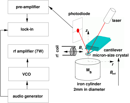
Figure 1: MRFMs are miniature version of the Faraday balance. The instrument fits between the poles of an electromagnet that generates a homogeneous static field $B_{ext}=$ 1T. A sample is affixed onto a micro-fabricated cantilever and placed in a field gradient $g=500$T/m produced by a 2 millimeter-size iron bar. The gradient serves to create a magnetic force on the spin system. The induced Å-scale bending of the cantilever is measured by a laser beam deflection on a photodiode. To increase the sensitivity, the nuclear magnetization is inverted periodically at 1.4kHz, a frequency that corresponds to the fundamental flexure mode of the cantilever. The induced vibration is monitored by a lock-in. The nuclear spin oscillations are obtained by cyclic adiabatic inversions using frequency modulated r.f. field produced by a VCO. The carrier is at the Larmor frequency of protons.

The setup is schematically represented in Fig.1. The experiment is performed at room temperature inside a vacuum cell (10^-2torr) constantly connected to the inlet of a rotary pump. The instrument guillous99 fits between the poles of an iron core electromagnet which produces a static magnetic field $B_{ext}\bm{k}$ along the $z$ axis. To the uniform field one adds a second inhomogeneous field with axial symmetry produced by a magnetized iron bar $8$mm in length and $1.9$mm in diameter. The polarization field experienced by the spin is $B_{0}=B_{ext}+B_{cyl}$, with $B_{0}=\bm{B}_{0}\cdot\bm{k}$ and $B_{cyl}=\bm{B}_{cyl}\cdot\bm{k}$. Near the symmetry axis, the instantaneous magnetic force acting on the sample is given by the expression gradient :

$$F(t)=\int_{V_{s}}M_{z}(\bm{r},t)\frac{\partial B_{cyl}}{\partial z}dV.$$ (1)

Here $M_{z}$ is the $z$ component of the bulk magnetization and $V_{s}$ is the volume of the sample. For small sample size, we make the approximation that the field gradient $g=\partial B_{cyl}/\partial z$ is uniform over $V_{s}$. A new length variable $\zeta=B_{0}(\bm{r})/g$ is defined so that a plane of constant $\zeta$ maps onto a surface (actually a paraboloid) of constant polarization field which also corresponds to a sheet where the spin have the same motion. A paraboloid of fixed $\zeta$ value, however, shifts axially away from the iron cylinder when $B_{ext}$ increases. In this experiment, the sample is placed 0.70mm above the iron cylinder and centered on the cylinder axis. At this distance, the calculated axial field gradient is $g=-$470T/m (see appendix A).

The mechanical force detection is obtained by measuring the elastic deformation along the $z$ axis of a micro-fabricated cantilever on which the sample is attached. In this orientation, the probe is sensitive to the longitudinal component of the nuclear magnetization in contrast with a standard coil detection. The cantilever equation of motion is represented by a damped harmonic oscillator with a single degree of freedom. The measurement technique uses the optical deflection of a 4 $\mu$W HeNe laser beam which reflects off the rear side of the cantilever onto a position-sensitive detector.

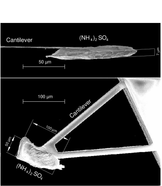
Figure 2: Images of a commercial Si₃N₄(amorphous) cantilever: A 7$\mu$m thick single-crystal of (NH₄)₂SO₄ sample is glued on the cantilever end with epoxy. The loaded cantilever has a resonance frequency of 1.4kHz, a spring constant of 0.008N/m and a quality factor of 4000 in vacuum. The estimated sample volume is $3.5\times 10^{-8}$cm³

Our test compound is (NH₄)₂SO₄. This non-magnetic insulator has a high proton density $d=6.4\times 10^{22}$ ¹H/cm³ and is in its paraelectric state above 223K. NMR measurements of the ¹H spin-lattice relaxation time at 300K in our powder aldrich give $T_{1z}\approx 5$s along the static field dooglav . The ¹H linewidth is 5G and the second moment is $M_{2}=4$G² at 295K richards60 . Our sample is a crystal cleaved to a platelet aspect ratio and glued with epoxy on the end of a commercial Si₃N₄ amorphous cantilever of spring constant $k=$0.008N/m as can been seen in Fig.2. After completing the assembly, the cantilever resonance frequency drops from 5.8kHz to 1.4kHz due to the sample mass stability . The quality factor of the loaded cantilever is $Q\approx$4000 in vacuum. From the electron microscopy images (Fig.2), the sample dimensions are approximately $100\times 50\times 7\mu$m³ with the smallest length (the thickness) oriented along the axial field. This represents a volume $V_{s}=3.5\times 10^{-8}$ cm³ or a mass $m=70$ng and corresponds to $N\approx 10^{15}$ protons. The temperature of the cantilever holder is stabilized around $+27^{\circ}$C during the measurement thermal . The nuclear magnetization at thermal equilibrium is expressed by the Curie law $\bm{M}_{0}=(d\mu_{n}^{2}B_{0}/k_{B}T)\,\bm{k}$, with $\mu_{n}=1.4\times 10^{-26}$J/T the proton magnetic moment, $T=300$K and $B_{0}=1.3$T the polarization field. This gives a magnetic moment $M_{0}V_{s}=2.3\times 10^{-16}$J/T.

In order to increase the sensitivity, $M_{z}$ is modulated at a frequency $\omega_{m}$ close to $\omega_{c}$, the frequency of the fundamental flexure mode of the cantilever. At the moment the optimal configuration uses cantilevers that have mechanical resonance frequencies in the audio range and Larmor frequencies $\omega_{0}$ which are several orders of magnitude larger (radio or microwave frequencies). Only two methods have been used to create an oscillatory force on the cantilever: cyclic saturation and cyclic adiabatic inversion. They are restricted respectively to compounds that have spin-lattice relaxation times $T_{1}$ either shorter or larger than the oscillation period of the cantilever.

In our case, the modulation of $\bm{M}$ is generated by a continuous-wave (c.w.) sequence that consists of periodic adiabatic fast passages abragam . The radio-frequency (r.f.) source is a 35-75MHz Voltage Controlled Oscillator (VCO). The r.f. output field is amplified up to 7W and fed into an impedance matched resonating circuit ($Q_{\mbox{rf}}\simeq 100$) tuned to a fixed frequency, 54.7MHz. A small coil (3 turns, 0.8mm in diameter) is in series with the tank circuit. The sample is 0.5mm away from this antenna. The nuclear spin are irradiated for a few seconds by a linearly polarized r.f. field $B_{x}=2B_{1}\cos\int_{0}^{t}\,\omega(t^{\prime})dt^{\prime}$ with $\omega(t)=\Omega\sin(\omega_{m}t)+\omega_{0}$, a sine-wave modulation of the r.f. frequency around the proton Larmor frequency $\omega_{0}=\gamma\,g\,\zeta_{0}$, where $\gamma/2\pi=4.258$kHz/G is the nuclear gyromagnetic ratio. The surface of constant $\zeta=\zeta_{0}$ is called the resonant sheet. The sinusoidal frequency modulation is started at a time $t=0$. In a transformation to a rotating coordinate system with an instantaneous angular velocity $\omega(t)\bm{k}$, the apparent magnetic field is:

$$\bm{B}_{e}(\zeta,t)=B_{1}\bm{i}+\left\{g\,\zeta-\frac{\omega(t)}{\gamma}\right\}\bm{k}.$$ (2)

$\theta$ is defined as the polar angle made by the apparent field with the external field. The magnetization, however, precesses about the direction $\bm{B}_{e}+\dot{\theta}/\gamma\,\bm{j}$, with $\dot{\theta}=\partial\theta/\partial t$ (see appendix B). A parameter for non-adiabaticity is defined with $\tan\alpha=\dot{\theta}/(\gamma\mid\bm{B}_{e}\mid)$ the angle between the two vectors. Provided that the adiabatic condition $\alpha\ll 1$ is satisfied, the spin system remains at all times in a state of internal equilibrium and $\bm{M}$ is parallel to $\bm{B}_{e}$ as required by Curie’s law. The longitudinal magnetization is $M_{z}(\zeta,t)=\mid\bm{M}\mid\cos\theta$, where

$$\cos\theta=\frac{g\,\zeta-\omega(t)/\gamma}{\sqrt{\left\{g\,\zeta-\omega(t)/\gamma\right\}^{2}+B^{2}_{1}}}.$$ (3)

For free spin, $\mid\bm{M}\mid$ is a constant of the motion abragam . This is no longer true in condensed matter because of spin-lattice relaxation. In our sample, however, the magnetization decay is slow compared to the modulation period. Under our measurement protocol, an extra defocusing originates from the lack of adiabaticity of the modulation. In a first step, these effects are neglected and they will be considered in a more detailed analysis deferred to a later section (see also the appendix B). At time $t=0$, $B_{1}$ is assumed to be turned on adiabatically with the sample initially in thermal equilibrium. In this case the norm $M$ reflects the state of the longitudinal magnetization immediately before the force measurement. During the c.w. sequence, the oscillatory movement of $M_{z}(t)$ comes from the $\cos\theta$ factor. The value is expanded in time series $\cos\theta\approx a_{0}+a_{1}\sin(\omega_{m}t)$ coherent with $a_{1}$ the first harmonic Fourier component zuger96 (higher harmonics have a negligible effect on the motion of the cantilever). Because of the large field inhomogeneities, the amplitude of oscillation depends on the location inside the sample. The resonant sheet, which is the paraboloid of constant $\zeta_{0}$, corresponds to the surface of maximum amplitude of oscillation. The spatial dependence of $a_{1}(\zeta)$ is the sensitivity profile. $\Gamma$ is the half width at half maximum of this bell-shaped curve. $\Gamma$ has the units of a distance and it defines the thickness of the slice probed. The amplitude of $\Gamma$ depends on both $\Omega$ and $B_{1}$ Gamma . The induced vibration is synchronously amplified by a lock-in technique through a single-pole low-pass linear filter of time constant $\tau_{l}$. For $\omega_{m}=\omega_{c}$, the lock-in signal grows exponentially (an exact expression will be given in equation (11)) to the asymptotic amplitude

$$A_{0}=\frac{1}{\sqrt{2}}\,\frac{Q\,g}{k}\,\int_{V_{s}}\,M_{0}\,a_{1}(\zeta)\,d\zeta.$$ (4)

In conclusion, the maximum amplitude of vibration achieved by the cantilever is proportional to the longitudinal magnetic moment inside the probed slice at the beginning of the c.w. sequence. In the ideal case of a uniform inversion of all spin inside the sample, the asymptotic amplitude would be $A_{\text{tot}}=QgM_{0}V_{s}/(k\sqrt{2})$.

Figure 3: (a) Vibration amplitude of the cantilever measured by the lock-in for a (NH₄)₂SO₄ crystal containing $10^{15}$ protons at 300K in $B_{ext}=0.9425$T. The trace corresponds to a single shot experiment with no averaging. The lock-in time constant is $\tau_{l}=0.3$s. (b) Details of the start and end of the c.w. sequence. The crystal is irradiated for 3s by a r.f. field of $B_{1}=10$G (upper panel). The bottom panel shows the frequency waveform applied to the VCO around $\omega_{0}/2\pi=54.7$MHz. The amplitude of the frequency modulation is $\Omega/2\pi=150$kHz. The width of the curve is the digitalization noise of the oscilloscope (not the phase noise).

In the upper panel of Fig.3 the time dependence of the lock-in output $A(t)$ is shown when the c.w. sequence is applied. The time delay between force measurements is set to 27s ($>5T_{1}$) to ensure a steady state magnetization close to the thermal equilibrium value. The lock-in time constant is $\tau_{l}=$0.3s which corresponds to an output noise of 4Å. The bottom panel of Fig.3 displays the time dependence of $B_{1}$ and $\omega$ at the beginning and end of the c.w. sequence. At the start, the amplitude of $B_{1}$ is turned on from 0 to 10G in 5ms when the frequency is well off-resonance, i.e. 400kHz below $\omega_{0}/2\pi$. The frequency is then ramped to resonance in 7ms. Finally, the frequency modulation of the r.f. field is applied for 3s with a deviation $\Omega/2\pi=150$kHz. For these settings, the calculated value of $\Gamma=7\mu$m is comparable to the sample thickness.

Since the r.f. tank circuit is tuned to a fixed frequency, the resonance is found by sweeping the external field $B_{ext}$. There is no spurious vibrations of the cantilever induced by the r.f. fields when $B_{ext}$ is outside the resonance range. Fig.3a shows the amplitude of the lock-in signal achieved in a one shot experiment at the resonance maximum, $B_{ext}=0.9425$T. The maximum vibration amplitude is around 40Å  which corresponds to a signal to noise ratio of 20dB. The shape of the lock-in signal $A(t)$ depends on the value $B_{ext}$ wago98 . For $B_{ext}$=0.9425T, i.e. $\zeta_{0}$ set at the middle of the sample thickness, no steady-state vibrations of the cantilever are induced by the c.w. sequence and the lock-in signal decays toward zero for long sequence. On the other hand, for $B_{ext}\neq 0.9425$T, an unbalanced partial repolarization of the magnetization occurs during each cycle and the lock-in signal decays to a finite value which changes sign for $B_{ext}$ smaller or larger than 0.9425T.

3 Relaxation measurements

Figure 4: The amplitude of the force signal (lock-in peak amplitude averaged over 1s around its maximum) is shown as a function of the width of a r.f. pulse applied 13ms before the c.w. sequence. Each point is the average of $16$ c.w. sequences. The solid line is proportional to a damped $\cos\varphi$ with $\varphi=\gamma\tau_{p}B_{1}$ the nutation angle. The 6.4W r.f. power during the pulse corresponds to a rotating field of $B_{1}=15$G at the sample location. The settings for the c.w. sequence are a r.f. field of 10G, $\Omega/2\pi=50$kHz and $\tau_{l}=100$ms. The inset is a schematic of the time dependence of $B_{1}$ (solid line) and $\omega$ (dashed line)

In this section the nuclear spin dynamics of our sample is measured by applying a series of r.f. pulses before the c.w. sequence described above.

In order to calibrate the strength of the r.f. field, a r.f. pulse of duration $\tau_{p}$ is applied, with an amplitude $B_{1}$, 13ms before the c.w. sequence. During this pulse, $\bm{M}_{0}$ rotates about $\bm{B}_{e}$ through an angle $\varphi$. The angle obtained at the end of the pulse is $\varphi=\gamma\mid\bm{B}_{e}\mid\tau_{p}$ wago96 ; wago98 . Within a few milli-seconds after the pulse, the nutated magnetization vector decays to its longitudinal component which then determines the amplitude of the maximum vibrations achieved by the cantilever during the force measurement. $B_{1}$ is set at maximum power, i.e. 6.4W, for the pulse. The c.w. sequence uses a 2.9W r.f. field. Fig.4 shows the lock-in output averaged over a 1s time interval around its peak amplitude. For spin that are at $\zeta_{0}$, the signal is proportional to $\cos\varphi$. The data are fitted by the functional form $\exp(-\tau_{p}/\tau)\cos(\gamma B_{1}\tau_{p})+b$. The period gives a calibration of the r.f. field strength at the sample location and we get $B_{1}=15$G during the pulse. The other fitting parameters are $\tau=43\pm 6\mu$s and a positive offset $b=3\pm 0.2$Å. The values of these last two parameters depend strongly on $B_{1}$. The positive offset $b$ is mainly due to the non-uniform field inside the sample relaxation . For ¹H away from $\zeta_{0}$, the direction of $\bm{B}_{e}$ is not exactly perpendicular to $\bm{k}$ and only a partial inversion of the $z$ component is obtained when $\varphi=\pi$. The decay of the magnetic moment fitted by $\tau$ is due to field inhomogeneity which causes a dephasing of the magnetization in the transverse plane tau .

Figure 5: Measurement of the transient shape of the spin-echo: A $\pi/2$-$\tau_{a}$-$\pi$ pulse sequence is used to form a spin echo. The transverse magnetization is measured with the combination of a $\pi/2$ pulse and the c.w. sequence. The amplitude of the force signal is shown as a function of $\tau_{a}+\tau_{b}$ with a fixed $\tau_{a}=17\mu$s. A r.f. field of $B_{1}=15$G is used for the pulses. The settings for the c.w. sequence are a r.f. field of 10G, $\Omega/2\pi=50$kHz and $\tau_{l}=100$ms. The solid line is the expected shape of the spin echo for a platelet of 6.5 $\mu$m thickness.

To study the transverse magnetization decay of ¹H wago98 a sequence of 3 pulses is used. A $\pi/2$ pulse is applied to the spin system, so that the magnetization at $\zeta_{0}$ is rotated to the transverse plane. After a fixed delay $\tau_{a}$, a $\pi$ pulse is applied to form a spin echo. Shortly after, a $\pi/2$ pulse takes an instant snap-shot of the transverse magnetization by rotating it along $\bm{k}$ and the frozen component is measured with the c.w. sequence. Varying the time delay $\tau_{b}$ between the last two pulses reconstructs the transient shape of the spin echo. Using the same settings as the earlier measurement, the widths of the $\pi/2$ and $\pi$ pulse are set to 3.8$\mu$s and 7.6$\mu$s respectively. The delay between the center of the first two pulses is $\tau_{a}=17\mu$s. In Fig.5, the lock-in peak (again averaged over 1s around its maximum) is shown as a function of $\tau_{a}+\tau_{b}$. As expected for a spin echo, the reconstructed transverse magnetization becomes refocused at a time $2\tau_{a}$.

Figure 6: Spin-spin relaxation time measurement: Normalized heights of the spin echo are displayed on a square-logarithmic scale as a function of $\tau_{a}+\tau_{b}$ with $\tau_{a}=\tau_{b}\$. The straight line is a fit with $\exp\left\{-(2\tau_{a}/T_{2})^{2}\right\}$ where $T_{2}=39\pm 1\mu$s.

With increasing spacing $\tau_{a}$ between pulses, the size of the spin echo signal decreases due to spin-spin relaxation. Using the same sequence as above, Fig.6 is a plot of the spin echo amplitude measured as a function of the time $2\tau_{a}$. The measured values are plotted on a $x^{2}$- $\log(y)$ scale and one finds that the data follow the relationship $\exp\left\{-(t/T_{2})^{2}\right\}$ with $T_{2}=39\pm 1\mu$s. With the inferred $T_{2}$, the shape of the echo in Fig.5 can be calculated taking into account the dipolar linewidth of the protons in our compound richards60 and the spatial dependence $a_{1}(\zeta)$. The solid line in Fig.5 is the best fit obtained for a sample thickness of $6.5\mu$m which is in good agreement with the value obtained on the image.

Figure 7: Measurement of the longitudinal magnetization recovery: The logarithmic of the normalized amplitude of the force signal is shown as a function of the interval $t$ between a saturation comb and the c.w. sequence. The solid line is a fit with a double exponential recovery which yields $T_{1s}=0.35\pm 0.03$s and $T_{1l}=5.4\pm 0.5$s. Each point is the average of 32 c.w. sequences. A r.f. field of $B_{1}=15$G is used for the comb. The settings for the cyclic adiabatic inversions are a r.f. field of 7G, $\Omega/2\pi=50$kHz and $\tau_{l}=100$ms. We make sure that there is no net repolarization of $M$ during the c.w. sequence.

The longitudinal magnetization recovery is now measured after a saturation comb fukushima . This protocol puts efficiently inhomogeneous spin systems in a well defined uniform state outside thermal equilibrium. The saturation comb is composed of three $\pi/2$ pulses spaced by 100$\mu$s. The c.w. sequence is applied at a variable delay (13ms $<t<$ 20s) after the comb. In order to obtain an intrinsic measurement of the relaxation, it is important to ensure that the sensitivity profile $a_{1}(\zeta)$ is exclusively included inside the sample section, otherwise a partial re-polarization of the magnetization occurs during the measurement cycle wago98 . For our settings, $\zeta_{0}$ is set exactly at the middle of the sample and $\Gamma=2.4\mu$m is smaller than the sample thickness. As before, the value plotted is the lock-in output averaged over a 1s time interval around its maximum. No signals are detected when $t=13$ms. On Fig.7, two relaxation times in the recovery process are clearly observed. The results are fitted with a double exponential ${\varrho}_{s}\left\{1-\exp(-t/T_{1s})\right\}+(1-{\varrho}_{s})\left\{1-\exp(-t/T_{1l})\right\}$ which gives ${\varrho}_{s}=49\pm 2$%, $T_{1s}=0.35\pm 0.03$s and $T_{1l}=5.4\pm 0.5$s. The value ${\varrho}_{s}$ does not correspond directly to the proportion of spin that have a short relaxation (${n}_{s}$) since the factor between $M_{z}$ and the lock-in amplitude is also a function of $T_{1}$.

Neutron diffraction studies schlemper66 of the (NH₄)₂SO₄ crystal structure show that there are two NH${}_{4}^{+}$ sites at room temperature surrounded respectively by five and six SO${}_{4}^{2-}$ ions. The protons of the two inequivalent ammonium ions are coupled via dipole-dipole interactions and the measured spin-lattice relaxation rate at 300K is an averaged value of the $T_{1}^{-1}$. In a variable temperature NMR measurements, O’Reilly and Tsang oreilly67 observe a single exponential ¹H relaxation process and analyze their $T_{1}$ results by the reorientation correlation times $\tau_{0}$ of the two distinctive NH${}_{4}^{+}$. At 300K, $1/\tau_{0}$ should be larger than the Larmor frequency and the rotation should be isotropic which means that $T_{1}$ should be independent of the orientation between the static field and the crystallographic axis of our sample. We suppose that our observed two $T_{1}$ processes might be due to water contamination inside the sample during its contact with air. The presence of H₂0 in the crystal lattice could decrease the reorientation correlation time of the ammonium ions, hence diminishing the protons $T_{1}$. The relatively high proportion of spin with short $T_{1}$ might be due to the exceptionally small thickness of our crystal (7 $\mu$m).

In order to check the later hypothesis, a conventional NMR measurement was performed by A. Dooglav with a 1T custom spectrometer. The sample consisted of $\sim 1$g of our sample ground to small particles with dimensions below $50\mu$m. In this fine powder sample, a double relaxation process is also observed with the following parameters $n_{s}=17\pm 5$%, $T_{1s}=0.37\pm 0.1$s and $T_{1l}=4.7\pm 0.2$s. This result is in sharp contrast with experiments performed on coarser grains, where only one relaxation is observed with $T_{1}=5.0\pm 0.2$s. The values of the two relaxation times are equal, within error bars, to the ones measured by MRFM. In addition, measurements were performed on the same $50\mu$m powder after two weeks of aging in air. It showed a rise of $n_{s}$ to $26\pm 3$% in the longitudinal magnetization recovery experiment. A standard spin-spin relaxation measurement on this powder seems also to indicate a double time $T_{2}$ with $n_{s}=20\pm 6$%, $T_{2s}=49\pm 12\mu$s and $T_{2l}=79\pm 1\mu$s.

Figure 8: Force signal as a function of $B_{ext}$: A saturation comb is applied 0.6s (closed circles) and 16s (open circles) before the c.w. sequence. The solid line is the expected profile for a parallelepiped sample of 7$\mu$m thickness within both the free spin and adiabatic approximations. The c.w. sequence uses a r.f. field of 7G, $\Omega/2\pi=25$kHz and $\tau_{l}=300$ms. The inset shows the transfer function that corresponds to these settings, $a_{1}$ is the spatial dependence of the sensitivity profile.

One corollary issue concerns the spatial distribution of each spin species inside the sample section. To perform this measurement, we record the amplitude of the lock-in signal as a function of $B_{ext}$ for two delays $t$ between the saturating comb and the c.w. sequence. By sweeping $B_{ext}$, the surface $\zeta_{0}$ is displaced to a different height in the sample. The force signal is then proportional to the density of spin around this location. In order to obtain a local measurement, the thickness $\Gamma$ of the slice probed is reduced by decreasing both $\Omega$ and $B_{1}$ during the c.w. sequence. The inset of Fig.8 shows the spatial dependence of the transfer function $a_{1}(\zeta)$ for our settings where $\Gamma$, the half width at half maximum, is $1.9\mu$m. By changing the delay $t$, the weight $\varrho_{s}$ of one spin species compared to the other can be varied. Qualitatively, the measurement protocol gives more weight to the spin species with short relaxation when the comb is close to the c.w. sequence. The obtained results are shown in Fig.8 for both $t=0.6$s (closed circles) and $t=16$s (open circles). A first look at the result indicates that a more rounded distribution is obtained for the $t=0.6$s data. The measurements, however, collected close to the edge of the sample are skewed by repolarization processes that modify the shape of the lock-in signal. Inside the bulk of the crystal $(0.942T\lesssim B_{ext}\lesssim 0.944T$), there is no clear evidence of a spatial modulation of one spin population compared to the other, e.g. a dip of the signal in the middle of the crystal. This result suggests that, within our resolution, the water contamination is uniform in the thickness. The solid line is a calculation of the expected profile for a parallelepiped sample of dimensions $100\times 50\times 7\mu$m³ within both the free spin and adiabatic approximations. In spite of the idealized model, the $t=16$s data (open circles) are well described by the calculated profile except for the high field range. The shoulder at $B_{ext}=0.946$T corresponds to the surface of the sample that has been glued with epoxy to the cantilever. We did not attempt to fit this part of the data. The observed step in the signal might be due to the protons in the epoxy. A small roll angle between the sample and the cantilever combined with the particular shape of our crystal is also consistent with the observed effect.

Although the data analyzed here-above ensure that two populations of spin with different NMR properties are present, their actual proportion is not quantitatively determined, as the actual values of the relaxation times influence the magnitude of the measured signal. For a better knowledge of the sensitivity of the technique to the measurement parameters, it is then necessary to perform quantitative analyses.

4 Quantitative measurements

In this section, we shall first calibrate the mechanical response of the cantilever and the mechanical noise. The time dependence $A(t)$ of the lock-in signal is calculated, taking into account relaxation processes and non-adiabatic effects. The experimental responses for different values of $B_{1}$ and $\Omega$ are compared with the calculations. This allows us to select an experimental condition for which non-adiabatic effects can be neglected. It is then shown that two relaxation times are indeed required to fit the time dependence of the observed lock-in signals, with values consistent with those obtained from $T_{1}$ data.

Figure 9: Noise vibration spectrum of the cantilever with the sample attached: The data is obtained in vacuum (10^-2torr) when no r.f. fields are applied. The lock-in time constant is $\tau_{l}$= 10s. The signal is the standard deviation of the lock-in output estimated over 100$\times\tau_{l}$. The cantilever holder temperature stability is better than $\pm 0.01^{\circ}$C during the measurement.

The $Q$ of the cantilever is first measured carefully through the noise vibration spectrum of the cantilever loaded with the sample in vacuum when the r.f. power is off. The lock-in time constant is set to $\tau_{l}$= 10s. An audio generator sweeps the lock-in reference around $\omega_{c}$. The plotted value in Fig.9 is the standard deviation of the lock-in signal estimated over 100$\times\tau_{l}$ (the mean lock-in signal is zero). During the whole experiment, the temperature stability of the cantilever is better than $\pm 0.01^{\circ}$C which guarantees that $\omega_{c}$ does not shift by more than $0.01$Hz. Fitting the squared amplitude with a Lorentzian hutter93 , one obtains the cantilever resonance frequency $\omega_{c}/2\pi=$ 1397.77Hz and quality factor $Q=4000$ (defined as the ratio of $\omega_{c}$ over the full width at half maximum of the power spectrum). Away from resonance, our sensitivity is limited by the noise of the detection electronics. It is several orders of magnitude smaller than the Å-scale motion of the cantilever at resonance and therefore it can be neglected. Near $\omega_{c}$, the cantilever motion consists of white noise amplified by a narrow-bandwidth mechanical resonator sidles99 . $\Delta\nu_{c}$ is the one-sided equivalent noise bandwidth (ENBW) of the mechanical resonator $\Delta\nu_{c}=\omega_{c}/8Q=0.27$Hz. The noise at the output of the lock-in is this narrow-band motion noise observed through a $RC$ filter of time constant $\tau_{l}=1/RC$ whose ENBW $\Delta\nu_{l}=1/4\tau_{l}=0.025$Hz. Exactly at resonance, the combined distribution gives an ENBW $\Delta\nu=(1/\Delta\nu_{c}+1/\Delta\nu_{l})^{-1}$=0.023 Hz. To convert our data to spectral density, the resonance amplitude in Fig.9 must be divided by $\sqrt{\Delta\nu}$. The measured noise spectral density is $\mathcal{A}=13$Å$/\sqrt{\mbox{Hz}}$. This figure also corresponds to the noise observed in Fig.3 where $\Delta\nu=0.20$Hz. The result has to be compared with the intrinsic correlation function for fluctuations of a Brownian particle harmonically bound to a single degree of freedom oscillator of spring constant $k$:

$$\langle AA(t)\rangle=\frac{4Qk_{B}T}{k\omega_{c}}.$$ (5)

Taking the square root of the above expression, one gets $\mathcal{A}_{T}=10$Å$/\sqrt{\mbox{Hz}}$ at $T=300$K which is in good agreement with our measured value. In conclusion, our dominant noise comes from the thermal vibration of the cantilever. From this result, one can estimate the smallest force detectable by the instrument in one shot $k\mathcal{A}/Q=$ 2$\times 10^{-15}$N$/\sqrt{\mbox{Hz}}$.

Figure 10: Time dependence of the lock-in signal: The trace is the average of 32 c.w. sequences with $\tau_{l}=30$ms. The c.w. sequence is composed of a r.f. field of 10G with $\Omega/2\pi=50$kHz. The solid line is the calculated vibration amplitude of a harmonic oscillator driven by a damped sinusoidal magnetic force with a decay time constant $\tau_{m}=2.2\pm 0.07$s. In this case, the predicted maximum signal is $A_{\text{peak}}=0.5A_{0}$ with $A_{0}=QF_{0}/k$.

In order to obtain a quantitative measurement of our force signal when the r.f. field is applied, a more detailed study of the time dependence of the lock-in signal $A(t)$ is needed. The length of the c.w. sequence is increased to 6s compared to Fig.3. Fig.10 is the average of the lock-in signal over 32 sequences using a short lock-in time constant of $\tau_{l}=30$ms. The striking feature of this plot is that the norm of the magnetization $\mid\bm{M}\mid$ decays during the c.w. sequence. We have checked that experimental perturbations such as the phase noise of the r.f. source are negligible in this case phase .

In the rotating frame, the magnetization tends to recover slowly towards a steady state value due to spin-lattice relaxation processes goldman . These relaxation processes are different from the relaxations measured in section 3 which are linked to the time dependence of the magnetization in the absence of r.f. fields. In addition, the lack of adiabaticity quantified by $\alpha\approx\dot{\theta}/\gamma B_{e}$ produces a precession movement around the locally changing effective field direction. This mistracking corresponds to a magnetization component perpendicular to the instantaneous precession axis $\bm{B}_{e}+\dot{\theta}/\gamma\,\bm{j}$ that relaxes due to spin-spin interactions. But in the limit where $\alpha\ll 1$ and $2\pi/\omega_{c}\ll T_{1}$, the decrease of $M$ after one cycle $\Delta=M(t+2\pi/\omega_{c})-M(t)$ is small. The value is calculated at the lowest order for one spin species (see appendix B).

$$\Delta \approx -M\left\{\int_{0}^{\frac{2\pi}{\omega_{c}}}\,\dot{\theta}(t)\int_{0}^{t}\,\dot{\theta}(t^{\prime})\exp\left(-\int_{t^{\prime}}^{t}\,\frac{1}{T_{1}^{+}}dt^{\prime\prime}\right)\right.$$ (6)

$$\hskip 85.35826pt\times\cos\left(\int_{t^{\prime}}^{t}\,\frac{\gamma B_{1}}{\sin\theta(t^{\prime\prime})}dt^{\prime\prime}\right)dt^{\prime}dt$$

$$\hskip 22.76219pt+\left.\int_{0}^{\frac{2\pi}{\omega_{c}}}\,\left(\frac{\cos^{2}\theta(t)}{T_{1z}}+\frac{\sin^{2}\theta(t)}{T_{1x}}\right)dt\right\}$$

$$+M_{0}\int_{0}^{\frac{2\pi}{\omega_{c}}}\,\frac{\cos\theta(t)}{T_{1z}}dt,$$

with $T_{1z}$ is the usual $T_{1}$ in the absence of r.f. field, $T_{1x}$ is the transversal spin-lattice relaxation and $1/T_{1}^{+}=(1/T_{1y}+\cos^{2}\theta/T_{1x}+\sin^{2}\theta/T_{1z})/2$. It was shown that the relaxation mechanisms in this compound are associated with the time varying field induced by the change in the NH${}_{4}^{+}$ orientation. For an exponential correlation function with correlation time $\tau_{0}$, $T_{1x}$ is expressed as a sum of the spectral density of these fluctuating fields $J^{(i)}(\omega)=\tau_{0}/(1+\omega^{2}\tau_{0})$ with an index $i$ that corresponds to the number of net spin flip: $1/T_{1x}=3/2\gamma^{4}\hbar^{2}I(I+1)/r^{6}(5/2J^{(1)}(\omega_{0})+1/4J^{(2)}(2\omega_{0})+1/4J^{(0)}(2\omega_{e}))$, with $\omega_{e}=\gamma B_{e}$. In the approximation for our compound that $\omega_{e}\tau_{0}\ll 1$, one obtains that $T_{1x}$ is independent of $\theta$ and $T_{1y}=T_{1x}$. Coming back to equation (6), one recognizes that the first integral is due to the finite value of the non-adiabaticity parameter $\alpha$ (see appendix B). The second represents the spin-lattice relaxation $T_{1\rho}$ in the rotating frame slichter . The last integral is the equilibrium magnetization that corresponds to the spin temperature in the rotating frame. $\tau$ and $M_{\text{eq}}$ are defined by rewriting the above expression in the form $\Delta/2\pi=-M/(\omega_{c}\tau)+M_{\text{eq}}/(\omega_{c}\tau)$. During the c.w. sequence, the oscillatory driving magnetic force is dampened and the instantaneous value is given by:

$$F(t)\approx g\sin(\omega_{m}t)\int_{V_{s}}\,a_{1}(\zeta)\,M(\zeta,t)\,d\zeta+\text{constant},$$ (7)

with

$$M(\zeta,t)=\left\{M_{\text{eq}}(\zeta)+\left\{M_{0}-M_{\text{eq}}(\zeta)\right\}\exp\left(\frac{-t}{\tau(\zeta)}\right)\right\}.$$ (8)

The integral in equation (7) relaxes approximately according to a single exponential towards its equilibrium value $m_{\text{eq}}=\int_{V_{s}}\,a_{1}(\zeta)M_{\text{eq}}(\zeta)d\zeta$ with an apparent characteristic time $\tau_{m}$. One notes that $m_{\text{eq}}=0$ by symmetry when $\zeta_{0}$ is centered at the middle of the sample $\zeta_{0}=\zeta_{m}$. The value of $m_{\text{eq}}$ is positive for $\zeta_{0}<\zeta_{m}$ and changes sign for $\zeta_{0}>\zeta_{m}$ wago98 . In the particular case where $m_{\text{eq}}=0$ and $\alpha\ll 1$, then it can be shown that the coefficient $\tau_{m}$ is bounded between $T_{1x}\leq\tau_{m}\leq T_{1z}$ verhagen99 .

The forced vibrations of an harmonic oscillator are given by the convolution product:

$$a(t)=\beta\,\int_{0}^{t}\,\frac{F(t^{\prime})}{k}\,{\exp\left\{-\frac{t-t^{\prime}}{\tau_{c}}\right\}}\sin\left\{\omega_{c}(t-t^{\prime})\right\}\,\omega_{c}\,dt^{\prime},$$ (9)

with $\beta=\left\{1+1/(4Q^{2})\right\}$ and $1/\tau_{c}$ the damping constant of the cantilever. In our experiment the external force is $F(t)=F_{0}\exp(-t/\tau_{m})\exp(i\omega_{m}t)$ for $m_{\text{eq}}=0$, with $F_{0}=kA_{0}/Q$ and $\tau_{m}$ the characteristic decay time of the magnetic force. ${a}(s)$ the Laplace transform of equation (9) is calculated in the complex plane:

$$\frac{k}{F_{0}}{a}(s)=\frac{\tau_{m}\left(4{Q}^{2}+1\right)}{\left(s\tau_{m}+1-i\tau_{m}\omega_{m}\right)\left\{(s\tau_{c}+1)^{2}+4Q^{2}\right\}}.$$ (10)

The response ${A}(t)$ of the lock-in is the imaginary part of the inverse Laplace transform $\cal{L}$${}^{-1}\left\{{a}(s+i\omega_{m})/(1+\tau_{l}s)\right\}$ with $\tau_{l}$ the lock-in time constant. An approximation can be obtained in the special case where $\omega_{m}=\omega_{c}$ in the limit $Q\gg 1$ and $\omega_{c}\gg(1/\tau_{m},1/\tau_{l})$.

$$\frac{{A}(t)}{A_{0}} \approx \hskip 7.11317pt\,\frac{1}{(1/\tau_{m}-1/\tau_{c})(\tau_{c}-\tau_{l})}\exp{\left(-\frac{t}{\tau_{c}}\right)}$$ (11)

$$+\,\frac{\tau_{m}/\tau_{c}}{(1/\tau_{c}-1/\tau_{l})(\tau_{l}-\tau_{m})}\exp{\left(-\frac{t}{\tau_{l}}\right)}$$

$$+\frac{\tau_{m}/\tau_{c}}{(1/\tau_{c}-1/\tau_{m})(\tau_{m}-\tau_{l})}\exp{\left(-\frac{t}{\tau_{m}}\right)}.$$

The sum of these three exponentials vanishes at $t=0$ and each term decays to zero with a different time constant at later time $t>0$. This leads to a peaked lock-in signal $A_{\text{peak}}$ whose amplitude and position depends on $\tau_{m}$ (for a fixed $\tau_{c}$ and $\tau_{l}$). At the end of the c.w. sequence in Fig.10 ($t>6$s), the free oscillations decay of the cantilever (time constant $\tau_{c}$) are observed. If one tries to fit the data with the above nonlinear form, $\tau_{m}=2.2\pm 0.07$s is obtained but the quality of the fit is not very good. Values of $\tau_{m}$ smaller than $T_{1x}=3.2$s have also been reported by Verhagen et al. verhagen99 and these findings were attributed to the phase noise of the r.f. source. However, when large modulation amplitude are employed for the c.w. sequence, such a fast force decay can also be consistent with a magnetization decrease due to a lack of adiabaticity.

Figure 11: (a) Measurements of the amplitude of the lock-in signal is shown as a function of the modulation amplitude for different strength of the r.f. field. The dashed lines are guides for the eye. The arrows indicate the limit of the adiabatic regime. The measurements are performed at $B_{ext}=0.9425$T. (b) Calculated amplitude of the lock-in signal obtained for a 7$\mu$m thick sample using equation (7). The parameters introduced in the model are $T_{1z}=4.9$s, $T_{1x}=T_{1y}=3.2$s and $T_{2}=40\mu$s (solid line) or $100\mu$s (dotted line).

To understand further the meaning of this fit parameter $\tau_{m}$, we plot in Fig.11a the lock-in peak amplitude measured for different values of $\Omega$ and $B_{1}$ when $B_{ext}=0.9425$T. The value of the non-adiabaticity parameter $\alpha$ increases along the abscissa axis. For a fixed $\Omega$ and $B_{1}$, the value of $\alpha$ oscillates with time and passes through a maximum, $\alpha_{\text{max}}=\Omega\omega_{m}/\gamma^{2}B_{1}^{2}$, at time a $t=0$ modulo $\pi/\omega_{m}$. Fig.11b shows the amplitude of the peak signal $A_{\text{peak}}$ predicted by equation (11) with $F(t)$ calculated from equation (7) using a sample thickness of 7$\mu$m. The results are normalized by $A_{\text{tot}}=QgM_{0}V_{s}/(k\sqrt{2})$ the amplitude associated with a uniform inversion of all spin inside the sample. The parameters introduced in the model are the values of the spin-lattice relaxation times measured on powder samples by conventional NMR with $T_{1z}=4.9$s along the static field and $T_{1x}=3.2$s along a 10G r.f. field, in the approximation that $T_{1y}=T_{1x}$. In our theoretical model, perturbation effects from the dipolar broadening are also introduced. They are approximated as a time independent local field of Lorentzian lineshape. The solid lines are the shape calculated with $T_{2}=40\mu$s (the dotted lines correspond to $T_{2}=100\mu$s).

The increase of the force signal at small $\Omega(\leq 50$kHz) corresponds to an increase of the modulated magnetic moment. A larger frequency deviation increases the width of the probed slice, $\Gamma$, and more protons oscillate at the frequency $\omega_{m}$. For both large $B_{1}\geq 14$G and large $\Omega\geq 150$kHz the amplitude of the signal eventually saturates when $\Gamma$ becomes larger than the sample thickness.

For $B_{1}=7$ and 10G, the deviation from the low $\Omega$-linear increase (indicated by the arrows) marks the cross-over from an adiabatic regime to a quasi-adiabatic one goldman . In our sample the threshold occurs at $\alpha_{\text{max}}=0.1$, in good agreement with the theoretical model. In the adiabatic regime ($\alpha_{\text{max}}<0.1$) the value of $\tau_{m}$ is determined by $T_{1\rho}$ effects, while in the quasi-adiabatic regime ($0.1<\alpha_{\text{max}}<1$) the magnetization decay $\tau_{m}$ becomes smaller than $T_{1x}$. The predicted position of this cross-over depends somewhat on the shape of the proton linewidth (dotted lines).

From the last discussion, one can conclude that the settings of Fig.10 correspond to a non-adiabatic parameter $\alpha_{\text{max}}=0.04$ well inside the adiabatic regime for our compound. It can then be inferred that the decrease of the force signal in Fig.10 is due to spin-lattice effects in the rotating frame and our fitted value of $\tau_{m}$ must be an average of the two $T_{1}$ reported in Fig.7.

Figure 12: Signal of Fig.10: The solid line is the response of an harmonic oscillator driven by two synchronous forces with short and long relaxations times $n_{s}A(t,\tau_{ms})+(1-n_{s})A(t,\tau_{ml})$. The best fit is obtained for $\tau_{ms}=0.55\pm 0.02$s, $\tau_{ml}=4.8\pm 0.2$s and $n_{s}=70$%. The height of the peak is $0.3A_{0}$. The dashed lines show the contribution of each spin species.

The time dependence of the lock-in signal is fitted with a double damped synchronous excitation of two spin populations with respectively short ($\tau_{ms}$) and long ($\tau_{ml}$) relaxation times. The nonlinear function $n_{s}A(t,\tau_{ms})+(1-n_{s})A(t,\tau_{ml})$ is used where $A(t)$ is given by equation (11). The best fit is obtained for $\tau_{ms}=0.55\pm 0.02$s, $\tau_{ml}=4.8\pm 0.2$s and $n_{s}=69\pm 1$%. The result is the solid line shown in Fig.12. The fit values obtained for the relaxation times are similar to those measured in the magnetization recovery experiment in Fig.7. On Fig.12 the separate contribution to the lock-in signal of each spin species (dashed lines) are shown. The maximum force signal of the two spin species occurs respectively 0.7s and 1.9s after the start of the c.w. sequence for the short and long $\tau_{m}$. It brings up the question on how to define the lock-in peak amplitude in the case of a sample containing two spin species. We recall that our definition of the force signal is the average of the lock-in peak amplitude over a 1s time interval around its maximum value. This approach gives approximately equal weights to both spin species in the measurement. One can also observe in Fig.12 that the height of the two peaks are approximately equal despite the fact that there is $2.3$ times more spin with short relaxation. As a matter of fact it can be shown that the mechanical detection is $2.4$ times more sensitive to spin that have a $4.8$s relaxation time compared to spin that have a 0.55s one. From this result, the value of the fit parameter ${\varrho}_{s}\approx 0.5$ in Fig.7 can be converted into the proportion of spin that have a short relaxation $n_{s}=2.4{\varrho}_{s}/\{(2.4-1){\varrho}_{s}+1\}=70$ %; a value that agrees well with the fit $n_{s}$ in Fig.12.

Finally, the expected amplitude of the force signal for our sample is calculated. Using equation (4), one gets a value of $A_{0}=100$Å  for the settings of the c.w. sequence used in Fig.12 ($B_{1}=10$G and $\Omega/2\pi=50$kHz). In Fig.12 the predicted maximum of the lock-in peak is $0.3A_{0}=30$Å  which is close to the experimentally measured value of 20Å. In conclusion, our measured amplitude of the peak lock-in signal is in good agreement with the theoretical prediction if the two spin-lattice relaxation times of the two spin species are taken into account. Other effects such as misalignment of the sample compared to the cylinder magnetic axis can account partially for a decrease of the signal (e.g. a small offset of 0.1mm from the axis decreases the amplitude of the lock-in signal by a factor of 2).

5 Conclusion

Measurement sequences combining fast adiabatic passages and pulses are reported. They allow us to measure $T_{1}$ and $T_{2}$ for microscopic samples using a mechanical detection. This has been applied to quantitative analyses of the detected signals for a 7$\mu$m thick sample of (NH₄)₂SO₄. The transverse relaxation $T_{2}$ has been found consistent with conventional NMR detection on a macroscopic sample. Our sample displays however two spin lattice relaxation times $T_{1s}=0.4$s and $T_{1l}=5$s. While the long $T_{1l}$ corresponds to that measured for coarse powder samples, the short $T_{1s}$ might be due to water contamination of our $7\mu$m thick crystal during its contact with air. This contamination is found to be uniform in the thickness of the sample. This large difference in $T_{1}$ values has allowed us to study the influence of the spin-lattice relaxation in the rotating frame on the measured time dependence of the lock-in signal, as well as the variation of signal intensity with increasing non-adiabaticity of the sweep sequence. A consistent analysis of all the experimental parameters has been proposed and will be quite useful in future quantitative investigations of MRFM signals. Our work also raises the problem on how to perform reliable spin lattice relaxation measurements at different locations in the sample. Our investigation is mainly restrained to the bulk, i.e. the middle of the sample. It is known that the time dependence of the lock-in signal (and thus the apparent relaxation times) depends strongly on the value of $B_{ext}$. These difficulties prevented us from interpreting quantitatively our results on the spatial distribution of the different spin densities close to the sample surface. This issue will be best resolved by performing a similar experiment on a hetero-layer sample of well-characterized composition.

Appendix A Inhomogeneous field

Near the axis, a uniformly magnetized ($M_{s}$) cylinder of length $l$ and diameter $\phi$ produces a field, whose component along $\bm{k}$, $B_{cyl}$, decays radially as

$$\frac{B_{cyl}(r,z)}{4\pi M_{s}}=\left\{b_{\frac{1}{2}}\left(\frac{z+l}{\phi}\right)-b_{\frac{1}{2}}\left(\frac{z}{\phi}\right)\right\}$$

$$+3\left\{b_{\frac{5}{2}}\left(\frac{z+l}{\phi}\right)-b_{\frac{5}{2}}\left(\frac{z}{\phi}\right)\right\}\frac{r^{2}}{\phi^{2}}+\mathcal{O}(r^{4}),$$ (A.1)

with $b_{a}(z)=z\left(1+4z^{2}\right)^{-a}$. The fields are expressed in cylindrical coordinates with the origin centered on the cylinder upper surface (see Fig.1). In our case $M_{s}$ is calculated from the applied field $B_{ext}$ needed to produce a resonance signal at the sample position, $z=0.70$mm. $B_{cyl}(0,z=0.70)=\omega_{0}/\gamma-B_{ext}=0.352$T is replaced in the above expression and one obtains $M_{s}\approx 1400$emu/cm³ for our iron. Using this result, the gradient $g=-470$T/m at the sample location can be calculated.

Appendix B Adiabaticity

The aim of this appendix B is to calculate the decrease of the magnetization due to the spin-lattice relaxation and the lack of adiabaticity. The solution below is proposed by M. Goldman. In the limit of strong r.f. fields (larger than the local field), one can neglect the spin-lattice relaxation of the dipolar energy expectation value. In the rotating frame, the time evolution of the different spin components are goldman :

$$\frac{\partial\langle I_{z}\rangle}{\partial t} = -\gamma B_{1}\langle I_{y}\rangle+\frac{\langle I_{0}\rangle-\langle I_{z}\rangle}{T_{1z}}$$ (B.1a)

$$\frac{\partial\langle I_{x}\rangle}{\partial t} = +\gamma B_{1}\cot\theta\langle I_{y}\rangle-\frac{\langle I_{x}\rangle}{T_{1x}}-\frac{i}{\hbar}\langle[\mathcal{H}_{Dz},I_{x}]\rangle$$ (B.1b)

$$\frac{\partial\langle I_{y}\rangle}{\partial t} = +\gamma B_{1}\left(\langle I_{z}\rangle-\cot\theta\langle I_{x}\rangle\right)-\frac{\langle I_{y}\rangle}{T_{1y}}-\frac{i}{\hbar}\langle[\mathcal{H}_{Dz},I_{y}]\rangle,$$ (B.1c)

with $\langle\bm{I}\rangle=\mbox{Tr}(\bm{I}\sigma)$ the expectation value of the magnetization, $\sigma$ the instantaneous density matrix in the rotating frame and $\mathcal{H}_{Dz}$ the secular part of the dipolar Hamiltonian. The commutator incorporates the local field contribution defined through $B_{L}^{2}=\text{Tr}(\mathcal{H}_{Dz}^{2})/\gamma^{2}\text{Tr}(I_{z}^{2})$. In our notation $\theta$ is the angle between the directions of the static and effective field, $B_{e}=B_{1}/\sin\theta$, with $B_{1}\cot\theta$ the projection along $\bm{k}$. Under r.f. irradiation, a new coordinate system $\{X,Y,Z\}$ is defined through a transformation by the unitary operator $\exp(-i\theta I_{y})$, a rotation around $y$ by $\theta$. In the doubly rotating frame the differential equations then become:

$$\frac{\partial\langle I_{Z}\rangle}{\partial t} = +c\frac{\langle I_{0}\rangle}{T_{1z}}-\left\{\frac{s^{2}}{T_{1x}}+\frac{c^{2}}{T_{1z}}\right\}\langle I_{Z}\rangle$$ (B.2a)

$$+\left(\dot{\theta}-cs\left\{\frac{1}{T_{1x}}-\frac{1}{T_{1z}}\right\}\right)\langle I_{X}\rangle$$

$$\frac{\partial\langle I_{X}\rangle}{\partial t} = -s\frac{\langle I_{0}\rangle}{T_{1z}}-\left(\dot{\theta}+cs\left\{\frac{1}{T_{1x}}-\frac{1}{T_{1z}}\right\}\right)\langle I_{Z}\rangle$$ (B.2b)

$$+\gamma\frac{B_{1}}{s}\langle I_{Y}\rangle-\left\{\frac{c^{2}}{T_{1x}}+\frac{s^{2}}{T_{1z}}\right\}\langle I_{X}\rangle$$

$$-\frac{3c^{2}-1}{2}\frac{i}{\hbar}\langle[\mathcal{H}_{DZ},I_{X}]\rangle$$

$$\frac{\partial\langle I_{Y}\rangle}{\partial t} = -\gamma\frac{B_{1}}{s}\langle I_{X}\rangle-\frac{\langle I_{Y}\rangle}{T_{1y}}-\frac{3c^{2}-1}{2}\frac{i}{\hbar}\langle[\mathcal{H}_{DZ},I_{Y}]\rangle,$$ (B.2c)

with $s=\sin\theta$ and $c=\cos\theta$. $\mathcal{H}_{DZ}$ is the doubly truncated part of the dipolar Hamiltonian that commutes with $I_{Z}$. The term $\dot{\theta}/\gamma\bm{j}$ is the inertia field due to the transformation to a time-dependent reference axis. In the adiabatic regime, defined by $\alpha=\dot{\theta}/(\gamma\ B_{e})\ll 1$, it can be shown that $\langle I_{X}\rangle=\langle I_{Y}\rangle=0$ and the first two terms of equation (B.2a) are the expression of the spin-lattice relaxation in the rotating frame for strong r.f. fields abragam ; slichter . This appendix seeks to evaluate the term proportional to $\langle I_{X}\rangle$ in equation (B.2a) that represents the decrease of $\langle I_{Z}\rangle$ due to the lack of adiabaticity. Our investigation will be restricted to the quasi-adiabatic regime goldman , where non-adiabaticity corrections might be dominant over $T_{1\rho}$ effects but $\alpha<1$. The equations of motion are expressed in terms of the raising and lowering operators $\langle I^{+}\rangle=\langle I_{X}\rangle+i\langle I_{Y}\rangle$ and $\langle I^{-}\rangle$ its complex conjugate. We suppose that $\gamma B_{e}\ll 1/\tau_{0}$, the reorientation correlation rate, for our compound which leads to $T_{1x}$ independent of $\theta$ and $T_{1y}\approx T_{1x}$. As a further simplification, spin-spin interactions are neglected and these effects will be calculated numerically later on. As a consequence, one has

$$\frac{\partial\langle I^{+}\rangle}{\partial t} \approx -i\gamma\frac{B_{1}}{s}\langle I^{+}\rangle-\frac{\langle I^{+}\rangle}{T_{1}^{+}}$$ (B.3)

$$-\left(\dot{\theta}+cs\left\{\frac{1}{T_{1x}}-\frac{1}{T_{1z}}\right\}\right)\langle I_{Z}\rangle-s\frac{\langle I_{0}\rangle}{T_{1z}},$$

with $1/T_{1}^{+}=(1/T_{1y}+c^{2}/T_{1x}+s^{2}/T_{1z})/2$. Furthermore, the period of the cyclic passage is much smaller than the spin-lattice relaxation times. Hence, both $1/T_{1z}$ and $1/T_{1x}$ are negligible compared to $\dot{\theta}$:

$$\frac{\partial\langle I^{+}\rangle}{\partial t}\approx-i\gamma\frac{B_{1}}{\sin\theta}\langle I^{+}\rangle-\frac{\langle I^{+}\rangle}{T_{1}^{+}}-\dot{\theta}\langle I_{Z}\rangle-\sin\theta\frac{\langle I_{0}\rangle}{T_{1z}},$$ (B.4)

which, upon integration, gives the result:

$$\langle I^{+}\rangle = -\int_{0}^{t}\,\left\{\dot{\theta}(t^{\prime})\langle I_{Z}\rangle+\sin\theta(t^{\prime})\frac{\langle I_{0}\rangle}{T_{1z}}\right\}$$ (B.5)

$$\times\exp\left\{-\int_{t^{\prime}}^{t}\,\frac{1}{T_{1}^{+}}+i\frac{\gamma B_{1}}{\sin\theta(t^{\prime\prime})}dt^{\prime\prime}\right\}dt^{\prime},$$

assuming that $\langle I^{+}\rangle=0$ at a time $t=0$. The expression for $\langle I^{-}\rangle$ is the complex conjugate of the above expression. For values of $t<T_{1}$, it is a good approximation to neglect $\langle I_{0}\rangle/T_{1z}$ compared to $\dot{\theta}\langle I_{Z}\rangle$ in the first bracket. Since the decay of $\langle I_{Z}\rangle$ is slow, it is replaced by a constant. Finally, the time variation of the longitudinal magnetization is given by:

$$\frac{\partial\langle I_{Z}\rangle}{\partial t} \approx -\langle I_{Z}\rangle\dot{\theta}(t)\int_{0}^{t}\,\dot{\theta}(t^{\prime})\exp\left(-\int_{t^{\prime}}^{t}\,\frac{1}{T_{1}^{+}}dt^{\prime\prime}\right)$$ (B.6)

$$\hskip 48.36967pt\times\cos\left(\int_{t^{\prime}}^{t}\,\frac{\gamma B_{1}}{\sin\theta(t^{\prime\prime})}dt^{\prime\prime}\right)dt^{\prime}$$

$$-\langle I_{Z}\rangle\left(\frac{\cos^{2}\theta(t)}{T_{1z}}+\frac{\sin^{2}\theta(t)}{T_{1x}}\right)$$

$$+\langle I_{0}\rangle\frac{\cos\theta(t)}{T_{1z}},$$

which has been used in equation (6) in the text. Although the general form of our final expression contains a $T_{1}^{+}$-exponential decay in the first integral, the decrease of the magnetization due to the quasi-adiabatic part of the c.w. sequence is unrelated to spin-lattice relaxation mechanisms. This is best seen in the free spin limit ($T_{1}\rightarrow\infty$), where the first term in equation (B.6) reduces to the integral form of the ordinary differential equation $\partial\langle\bm{I}\rangle/\partial t=\gamma\langle\bm{I}\rangle\times\bm{B_{e}}$, an equation of motion that preserves the norm of the magnetization. Our above solution expresses the decrease of $\langle I_{Z}\rangle$ with the set of initial condition $\langle I^{+}\rangle=0$ at $t=0$. Without local field effects, the free spin solution would eventually reach a finite “steady state” and for these large time scales, it is then important to take into account spin-spin interactions.

These interactions are best seen in another rotating frame $\{X^{\prime},Y^{\prime},Z^{\prime}\}$ where the direction $Z^{\prime}$ is aligned along the instantaneous axis of precession of the magnetization. The new system of differential equations is obtained by applying the unitary transformation $\exp(-i\alpha I_{X})$ to the equation system (B.2). Here second order corrections are examined and a more detailed analysis should take care of the new inertia field $\dot{\alpha}$. In this triply rotating coordinate system, the relaxation mechanisms along the $X^{\prime}$ and $Y^{\prime}$ directions are dominated by local field effects and these have a characteristic time of the order of $T_{2}\sim 40\mu$s in our sample. The exact expression is more complicated because the local field in the triply rotating frame oscillates with time. The system of differential equations is solved numerically in the approximation that the local field is time independent and of Lorentzian lineshape. The result is compared with the expression obtained in equation (6). The two calculated values of $\langle I_{Z^{\prime}}\rangle$ ($\approx\langle I_{Z}\rangle$ when $\alpha<1$) are close in both cases after one passage ($\pi/\omega_{m}$). The main difference occurs after several passages: when local field effects are included, the amplitude $\langle I_{Z^{\prime}}\rangle$ decays toward zero and the expectation value of the norm of the magnetization follows approximately the instantaneous value of $\langle I_{Z^{\prime}}\rangle$.

References

- (1) A. Abragam, Principles of Nuclear Magnetism (Oxford University Press, 1961).
- (2) J. A. Sidles, Appl. Phys. Lett. 58, 2854 (1991).
- (3) J. A. Sidles, Phys. Rev. Lett. 68, 1124 (1992).
- (4) J. A. Sidles and D. Rugar, Phys. Rev. Lett. 70, 3506 (1993).
- (5) J. A. Sidles, J. L. Garbini, K. J. Bruland, D. Rugar, O. Züger, S. Hoen, and C. S. Yannoni, Rev. Mod. Phys. 67, 249 (1995).
- (6) D. Rugar, C. S. Yannoni, and J. A. Sidles, Nature 360, 563 (1992).
- (7) D. Rugar, O. Züger, S. Hoen, C. S. Yannoni, H. M. Vieth, and R. D. Kendrick, Science 264, 1560 (1994).
- (8) Z. Zhang, P. C. Hammel, and P. E. Wigen, Appl. Phys. Lett. 68, 2005 (1996).
- (9) O. Züger and D. Rugar, Appl. Phys. Lett. 63, 2496 (1993).
- (10) P. C. Hammel, Z. Zhang, G. J. Moore, and M. L. Roukes, J. Low Temp. Phys. 101, 59 (1995).
- (11) O. Züger, S. T. Hoen, C. S. Yannoni, and D. Rugar, J. Appl. Phys. 79, 1881 (1996).
- (12) A. Schaff and W. S. Veeman, Appl. Phys. Lett. 70, 2598 (1997).
- (13) B. J. Suh, P. C. Hammel, Z. Zhang, and M. M. M. et al., J. Vac. Sci. and Technol. B 16, 2275 (1998).
- (14) C. Ascoli, P. Baschieri, C. Frediani, L. Lenci, M. Martinelli, G. Alzetta, R. M. Celli, and L. Pardi, Appl. Phys. Lett. 69, 3920 (1996).
- (15) K. Wago, O. Züger, R. Kendrick, C. S. Yannoni, and D. Rugar, J. Vac. Sci. and Technol. B 14, 1197 (1996).
- (16) K. Wago, O. Züger, J. Weneger, R. Kendrick, C. S. Yannoni, and D. Rugar, Rev. Sci. Instrum. 68, 1823 (1997).
- (17) K. Wago, D. Botkin, C. S. Yannoni, and D. Rugar, Phys. Rev. B 57, 1108 (1998).
- (18) K. Wago, D. Botkin, C. S. Yannoni, and D. Rugar, Appl. Phys. Lett. 72, 2757 (1998).
- (19) K. J. Bruland, W. M. Dougherty, J. L. Garbini, J. A. Sidles, and S. H. Chao, J. Appl. Phys. 73, 3159 (1998).
- (20) A. Schaff and W. S. Veeman, J. Magn. Res. 126, 200 (1997).
- (21) R. Verhagen, C. W. Hilbers, A. P. M. Kentgens, L. Lenci, R. Groeneveld, A. Wittli, and H. van Kempen, Phys. Chem. Chem. Phys. 1, 4025 (1999).
- (22) S. R. Miller, R. Blinc, M. Brenman, and J. S. Waugh, Phys. Rev. 126, 528 (1962).
- (23) D. E. O’Reilly and T. Tsang, J. Chem. Phys. 46, 1291 (1967).
- (24) S. Guillous and O. Klein (to be published).
- (25) Near the symmetry axis, .
- (26) 99.999% purity (Aldrich).
- (27) The value is measured in a 1T field using a coil detection (A. Dooglav). In this experiment, the powder is made of coarse grains.
- (28) R. E. Richards and T. Scaefer, Trans. Faraday Soc. 57, 210 (1961).
- (29) The sample mass and shape are stable for the duration of the experiment.
- (30) Using the static flexion of the cantilever as a temperature sensor, we estimate to C the elevation of the sample temperature during the r.f.-irradiation.
- (31) We can do this approximation because all slices are phase coherent.
- (32) The width of the probed slice is proportional to .
- (33) The fast relaxation can also partially explain the positive offset .
- (34) In the limit thickness, equals to abragam .
- (35) E. Fukushima and S. B. W. Roeder, Experimental pulse NMR (Addison-Wesley, 1981).
- (36) E. O. Schlemper and W. C. Hamilton, J. Chem. Phys. 44, 4498 (1966).
- (37) J. L. Hutter and J. Bechhoefer, Rev. Sci. Instrum. 64, 1868 (1993).
- (38) Comments about MRFM noise can be found in http://weber.u.washington.edu/sidles/.
- (39) The phase noise of our setup is estimated from fast adiabatic passage measurements on de-ionized H2O in a 1T field with a coil detection and comparing the apparent obtained with the VCO and a Marconi 2023 synthesizer.
- (40) M. Goldman, Spin temperature and Nuclear Magnetic Resonance in solids (Oxford University Press, 1970).
- (41) C. P. Slichter, Principles of Magnetic Resonance (Springer, Berlin, Heidelberg, New York, 1996), 3rd ed.