Randomly dilute spin models: a six-loop field-theoretic study.

Abstract

We consider the Ginzburg-Landau $MN$-model that describes $M$ $N$-vector cubic models with $O(M)$-symmetric couplings. We compute the renormalization-group functions to six-loop order in $d=3$. We focus on the limit $N\to 0$ which describes the critical behaviour of an $M$-vector model in the presence of weak quenched disorder. We perform a detailed analysis of the perturbative series for the random Ising model $(M=1)$. We obtain for the critical exponents: $\gamma=1.330(17)$, $\nu=0.678(10)$, $\eta=0.030(3)$, $\alpha=-0.034(30)$, $\beta=0.349(5)$, $\omega=0.25(10)$. For $M\geq 2$ we show that the $O(M)$ fixed point is stable, in agreement with general non-perturbative arguments, and that no random fixed point exists.

I Introduction.

The critical behavior of systems with quenched disorder is of considerable theoretical and experimental interest. A typical example is obtained by mixing an (anti)-ferromagnetic material with a non-magnetic one, obtaining the so-called dilute magnets. These materials are usually described in terms of a lattice short-range Hamiltonian of the form

$${\cal H}_{x}=-J\,\sum_{<ij>}\rho_{i}\,\rho_{j}\;\vec{s}_{i}\cdot\vec{s}_{j},$$ (1)

where $\vec{s}_{i}$ is an $M$-component spin and the sum is extended over all nearest-neighbor sites. The quantities $\rho_{i}$ are uncorrelated random variables, which are equal to one with probability $x$ (the spin concentration) and zero with probability $1-x$ (the impurity concentration). The pure system corresponds to $x=1$. One considers quenched disorder, since the relaxation time associated to the diffusion of the impurities is much larger than all other typical time scales, so that, for all practical purposes, one can consider the position of the impurities fixed. For sufficiently low spin dilution $1-x$, i.e. as long as one is above the percolation threshold of the magnetic atoms. the system described by the Hamiltonian ${\cal H}_{x}$ undergoes a second-order phase transition at $T_{c}(x)<T_{c}(x=1)$ (see e.g. Ref. [1] for a review).

The relevant question in the study of this class of systems is the effect of the disorder on the critical behavior. The Harris criterion [2] states that the addition of impurities to a system which undergoes a second-order phase transition does not change the critical behavior if the specific-heat critical exponent $\alpha_{\rm pure}$ of the pure system is negative. If $\alpha_{\rm pure}$ is positive, the transition is altered. Indeed, in disordered systems the exponent $\nu$ satisfies the inequality $\nu\geq 2/d$ [3, 4] — this fact has been questioned however in Refs. [5, 6] — and therefore, by hyperscaling, $\alpha_{\rm random}$ is negative. Thus, if $\alpha_{\rm pure}$ is positive, $\alpha_{\rm random}$ differs from $\alpha_{\rm pure}$, so that the pure system and the dilute one have a different critical behavior. In pure $M$-vector models with $M>1$, the specific-heat exponent $\alpha_{\rm pure}$ is negative; therefore, according to the Harris criterion, no change in the critical asymptotic behavior is expected in the presence of weak quenched disorder. This means that in these systems disorder leads only to irrelevant scaling corrections. Three-dimensional Ising systems are more interesting, since $\alpha_{\rm pure}$ is positive. In this case, the presence of quenched impurities leads to a new universality class.

Theoretical investigations, using approaches based on the renormalization group [7, 8, 9, 10, 11, 12, 13, 14, 15, 16, 17, 18, 19, 20, 21, 22, 23, 24, 25, 26, 27, 28, 29, 30, 31, 32, 33, 34, 35, 36, 37], and numerical Monte Carlo simulations [38, 39, 40, 41, 42, 43, 44, 45, 46, 47, 48, 49, 50, 51, 52], support the existence of a new random Ising fixed point describing the critical behavior along the $T_{c}(x)$ line: the critical exponents are dilution independent (for sufficiently low dilution) and different from those of the pure Ising model.

Experiments confirm this picture. Cristalline mixtures of an Ising-like uniaxial antiferromagnet with short-range interactions (e.g. FeF₂, MnF₂) with a nonmagnetic material (e.g. ZnF₂ ) provide a typical realization of the random Ising model (RIM) (see e.g. Refs. [53, 54, 55, 56, 57, 58, 59, 60, 61, 62, 63, 64, 65, 66, 67, 68, 69]). Some experimental results are reported in Table I. This is not a complete list, but it gives an overview of the experimental state of the art. Other experimental results can be found in Refs. [1, 36]. The experimental estimates are definitely different from the values of the critical exponents for pure Ising systems, which are (see Ref. [70] and references therein) $\gamma=1.2371(4)$, $\nu=0.63002(23)$, $\alpha=0.1099(7)$, and $\beta=0.32648(18)$. Moreover, they appear to be independent of the concentration. We mention that in the presence of an external magnetic field along the uniaxial direction, dilute Ising systems present a different critical behavior, equivalent to that of the random-field Ising model [71]. This is also the object of intensive theoretical and experimental investigations (see e.g. Refs. [72, 73]).

Several experiments also tested the effect of disorder on the $\lambda$-transition of ⁴He that belongs to the $XY$ universality class, corresponding to $M=2$ [74, 75, 76, 77, 78, 79]. They studied the critical behaviour of ⁴He completely filling the pores of porous gold or Vycor glass. The results indicate that the transition is in the same universality class of the $\lambda$-transition of the pure system in agreement with the Harris criterion [80].

TABLE I.: Experimental estimates of the critical exponents for systems in the RIM universality class.

Ref.	material	concentration	$\gamma$	$\nu$	$\alpha$	$\beta$
[56]	FexZn1-xF2	$x=0.46$	$1.33(2)$	$0.69(3)$
[58]	MnxZn1-xF2	$x=0.75$	$1.364(76)$	$0.715(35)$
[60]	FexZn1-xF2	$x=0.9$				$0.350(9)$
[61]	MnxZn1-xF2	$x=0.40,0.55,0.83$			$-0.09(3)$
[62]	MnxZn1-xF2	$x=0.5$				$0.33(2)$
[66]	FexZn1-xF2	$x=0.5$				$0.36(2)$
[68]	FexZn1-xF2	$x=0.93$			$-0.10(2)$
[69]	FexZn1-xF2	$x=0.93$	$1.34(6)$	$0.70(2)$

The starting point of the field-theoretic approach to the study of ferromagnets in the presence of quenched disorder is the Ginzburg-Landau-Wilson Hamiltonian [12]

$${\cal H}=\int d^{d}x\left\{{1\over 2}(\partial_{\mu}\phi(x))^{2}+{1\over 2}r\phi(x)^{2}+{1\over 2}\psi(x)\phi(x)^{2}+{1\over 4!}g_{0}\left[\phi(x)^{2}\right]^{2}\right\},$$ (2)

where $r\propto T-T_{c}$, and $\psi(x)$ is a spatially uncorrelated random field with Gaussian distribution

$$P(\psi)={1\over\sqrt{4\pi}w}\exp\left[-{\psi^{2}\over 4w}\right].$$ (3)

We consider quenched disorder. Therefore, in order to obtain the free energy of the system, we must compute the partition function $Z(\psi,g_{0})$ for a given distribution $\psi(x)$, and then average the corresponding free energy over all distributions with probability $P(\psi)$. By using the standard replica trick, it is possible to replace the quenched average with an annealed one. First, the system is replaced by $N$ non-interacting copies with annealed disorder. Then, integrating over the disorder, one obtains the Hamiltonian [12]

$${\cal H}_{MN}=\int d^{d}x\left\{\sum_{i,a}{1\over 2}\left[(\partial_{\mu}\phi_{a,i})^{2}+r\phi_{a,i}^{2}\right]+\sum_{ij,ab}{1\over 4!}\left(u_{0}+v_{0}\delta_{ij}\right)\phi^{2}_{a,i}\phi^{2}_{b,j}\right\}$$ (4)

where $a,b=1,...M$ and $i,j=1,...N$. The original system, i.e. the dilute $M$-vector model, is recovered in the limit $N\rightarrow 0$. Note that the coupling $u_{0}$ is negative (being proportional to minus the variance of the quenched disorder), while the coupling $v_{0}$ is positive.

In this formulation, the critical properties of the dilute $M$-vector model can be investigated by studying the renormalization-group flow of the Hamiltonian (4) in the limit $N\rightarrow 0$, i.e. of ${\cal H}_{M0}$. One can then apply conventional computational schemes, such as the $\epsilon$-expansion, the fixed-dimension $d=3$ expansion, the scaling-field method, etc… In the renormalization-group approach, if the fixed point corresponding to the pure model is unstable and the renormalization-group flow moves towards a new random fixed point, then the random system has a different critical behavior.

It is important to note that in the renormalization-group approach one assumes that the replica symmetry is not broken. In recent years, however, this picture has been questioned [86, 87, 88] on the ground that the renormalization-group approach does note take into account other local minimum configurations of the random Hamiltonian (2), which may cause the spontaneous breaking of the replica symmetry. In this paper we assume the validity of the standard renormalization-group approach, and simply consider the Hamiltonian (4) for $N=0$.

For generic values of $M$ and $N$, the Hamiltonian ${\cal H}_{MN}$ describes $M$ coupled $N$-vector models and it is usually called $MN$ model [13]. ${\cal H}_{MN}$ has four fixed points: the trivial Gaussian one, the O($M$)-symmetric fixed point describing $N$ decoupled $M$-vector models, the O($MN$)-symmetric and the mixed fixed point. The Gaussian one is never stable. The stability of the other fixed points depends on the values of $M$ and $N$ (see e.g. Ref. [13] for a discussion). The stability properties of the decoupled O($M$) fixed point can be inferred by observing that the crossover exponent associated with the O($MN$)-symmetric interaction (with coupling $u_{0}$) is related to the specific-heat critical exponent of the O($M$) fixed point [89, 13]. Indeed, at the O($M$)-symmetric fixed point one may interpret ${\cal H}_{MN}$ as the Hamiltonian of $N$ $M$-vector systems coupled by the O($MN$)-symmetric term. But this interaction is the sum of the products of the energy operators of the different $M$-vector models. Therefore, at the O($M$) fixed point, the crossover exponent $\phi$ associated to the O($MN$)-symmetric quartic term should be given by the specific-heat critical exponent $\alpha_{M}$ of the $M$-vector model, independently of $N$. This argument implies that for $M=1$ (Ising-like systems) the pure Ising fixed point is unstable since $\phi=\alpha_{I}>0$, while for $M>1$ the O($M$) fixed point is stable given that $\alpha_{M}<0$. This is a general result that should hold independently of $N$.

For the quenched disordered systems described by the Hamiltonian ${\cal H}_{M0}$, the physically relevant region for the renormalization-group flow corresponds to negative values of the coupling $u$ [12, 11]. Therefore, for $M>1$ the renormalization group flow is driven towards the pure O($M$) fixed point, and the quenched disorder yields correction to scaling proportional to the spin dilution and to $|t|^{\Delta_{r}}$ with $\Delta_{r}=-\alpha_{M}$. Note that for the physically interesting two- and three-vector models the absolute value of $\alpha_{M}$ is very small: $\alpha_{2}\simeq-0.013$ (see e.g. the recent results of Refs. [81, 90, 91, 82]) and $\alpha_{3}\simeq-0.12$ (see e.g. [90, 92]). Thus disorder gives rise to very slowly-decaying scaling corrections. For Ising-like systems, the pure Ising fixed point is instead unstable, and the flow for negative values of the quartic coupling $u$ leads to the stable mixed or random fixed point which is located in the region of negative values of $u$. The above picture emerges clearly in the framework of the $\epsilon$-expansion, although for the Ising-like systems the RIM fixed point is of order $\sqrt{\epsilon}$ [10] rather than $\epsilon$.

The other fixed points of the Hamiltonian ${\cal H}_{M0}$ are located in the unphysical region $u>0$. Thus, they are not of interest for the critical behavior of randomly dilute spin models. For the sake of completeness, we mention that for $M>1$ the mixed fixed point is in the region of positive $u$ and is unstable [13]. The last fixed point is on the positive $v=0$ axis, is stable and corresponds to the $(MN)$-vector theory for $N\rightarrow 0$. It is therefore in the same universality class of the self-avoiding walk model (SAW). Figure 1 sketches the flow diagram for Ising ($M=1$) and multicomponent ($M>1$) systems.

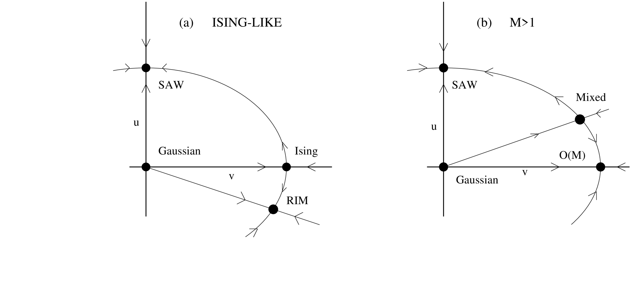
FIG. 1.: Renormalization-group flow in the coupling plane $(u,v)$ for (a) Ising ($M=1$) and (b) $M$-component ($M>1$) systems. Here $N=0$.

The Hamiltonian ${\cal H}_{MN}$ has been the object of several field-theoretic studies, especially for $M=1$, the case that describes the RIM. Several computations have been done in the framework of the $\epsilon$-expansion [93] and of the fixed-dimension $d=3$ expansion [94]. In these approaches, since field-theoretic perturbative expansions are asymptotic, the resummation of the series is essential to obtain accurate estimates of physical quantities. For pure systems described by the Ginzburg-Landau-Wilson Hamiltonian one exploits the Borel summability [95] of the fixed-dimension expansion (for which Borel summability is proved) and of the $\epsilon$-expansion (for which Borel summability is conjectured), and the knowledge of the large-order behavior of the series [96, 97]. Resummation procedures using these properties lead to accurate estimates (see e.g. Refs. [98, 99, 100, 90, 92]).

Much less is known for the quenched disordered models described by ${\cal H}_{M0}$. Indeed, the analytic structure of the corresponding field theory is much more complicated. The zero-dimensional model has been investigated in Ref. [101]. They analyze the large-order behavior of the double expansion in the quartic couplings $u$ and $v$ of the free energy and show that the expansion in powers of $v$, keeping the ratio $\lambda=-u/v$ fixed, is not Borel summable. In Ref. [102], it is shown that the non-Borel summability is a consequence of the fact that, because of the quenched average, there are additional singularities corresponding to the zeroes of the partition function $Z(\psi,g_{0})$ obtained from the Hamiltonian (2). Recently the problem has been reconsidered in Ref. [103]. In the same context of the zero-dimensional model, it has been shown that a more elaborate resummation gives the correct determination of the free energy from its perturbative expansion. The procedure is still based on a Borel summation, which is performed in two steps: first, one resums in the coupling $v$ each coefficient of the series in $u$; then, one resums the resulting series in the coupling $u$. There is no proof that this procedure works also in higher dimensions, since the method relies on the fact that the zeroes of the partition function stay away from the real values of $v$. This is far from obvious in higher-dimensional systems.

At present, the most precise field-theoretic results have been obtained using the fixed-dimension expansion in $d=3$. Several quantities have been computed: the critical exponents [18, 20, 23, 24, 25, 27, 32, 34, 35, 37], the equation of state [28] and the hyperuniversal ratio $R^{+}_{\xi}$ [28, 33]. The most precise estimates of the critical exponents for the RIM have been obtained from the analysis of the five-loop fixed-dimension expansion, using Padé-Borel-Leroy approximants [37]. In spite of the fact that the series considered are not Borel summable, the results for the critical exponents are stable: they do not depend on the order of the series, the details of the analysis, and, as we shall see, are in substantial agreement with our results obtained following the precedure proposed in Ref. [103]. This fact may be explained by the observation of Ref. [101] that the Borel resummation applied in the standard way (i.e. at fixed $v/u$) gives a reasonably accurate result for small disorder if one truncates the expansion at an appropriate point, i.e. for not too long series.

The $MN$ model has also been extensively studied in the context of the $\epsilon$-expansion [7, 9, 10, 11, 12, 13, 14, 15, 16, 19, 21, 22, 26, 30]. The critical exponents have been computed to three loops for generic values of $M$, $N$ [22] and to five loops for $M=1$ [104]. Several studies also considered the equation of state [14, 19, 26] and the two-point correlation function [14, 21]. In spite of these efforts, studies based on the $\epsilon$-expansion have been not able to go beyond a qualitative description of the physics of three-dimensional randomly dilute spin models. The $\sqrt{\epsilon}$-expansion [10] turns out not to be effective for a quantitative study of the RIM (see e.g. the analysis of the five-loop series done in Ref. [30]). A strictly related scheme is the so-called minimal-subtraction renormalization scheme without $\epsilon$-expansion [105]. The three-loop [29] and four-loop [31, 34, 36] results are in reasonable agreement with the estimates obtained by other methods. At five loops, however, no random fixed point can be found [36] using this method. This negative result has been interpreted as a consequence of the non-Borel summability of the perturbative expansion. In this case, the four-loop series could represent the “optimal” truncation. We also mention that the Hamiltonian (4) for $M=1$ and $N\rightarrow 0$ has been studied by the scaling-field method [17].

The randomly dilute Ising model (1) has been investigated by many numerical simulations (see e.g. Refs. [38, 39, 40, 41, 42, 43, 44, 45, 46, 47, 48, 49, 50, 51]). The first simulations were apparently finding critical exponents depending on the spin concentration. It was later remarked [48, 29] that this could be simply a crossover effect: the simulations were not probing the critical region and were computing effective exponents strongly biased by the corrections to scaling. Recently, the critical exponents have been computed [51] using finite-size scaling techniques. They found very strong corrections to scaling, decaying with a rather small exponent $\omega\simeq 0.37(6)$, — correspondingly $\Delta=\omega\nu=0.25(4)$ — which is approximately a factor of two smaller than the corresponding pure-case exponent. By taking into proper account the confluent corrections, they were able to show that the critical exponents are universal with respect to variations of the spin concentration in a wide interval above the percolation point. Their final estimates are reported in Table II.

In this paper we compute the renormalization-group functions of the generic $MN$ model to six loops in the framework of the fixed-dimension $d=3$ expansion. We extend the three-loop series of Ref. [23] and the expansions for the cubic model ($M=1$) reported in Ref. [37] (five loops) and Ref. [92] (six loops). We will focus here on the case $N=0$ corresponding to disordered dilute systems. Higher values of $N$ are of interest for several types of magnetic and structural phase transitions and will be discussed in a separate paper. For $M=1$ and $N\geq 2$ the six-loop series have already been analyzed in Ref. [92] where we investigated the stability of the $O(N)$-symmetric point in the presence of cubic interactions. We should mention that two-loop and three-loop series for the $MN$ model in the fixed dimension expansion for generic values of $d$ have been reported in Refs. [27, 32].

TABLE II.: Best theoretical estimates of the critical exponents for the RIM universality class. We report results for the massive scheme in fixed dimension $d=3$ (“$d=3$ exp.”), the minimal subtraction scheme without $\epsilon$-expansion (“$d=3$ MS”), and the best Monte Carlo (“MC”) results.

	Method	$\gamma$	$\nu$	$\eta$	$\omega$
This work	$d=3$ exp. $O(g^{6})$	1.330(17)	0.678(10)	0.030(3)	0.25(10)
Ref. [37], 2000	$d=3$ exp. $O(g^{5})$	1.325(3)	0.671(5)	0.025(10)	0.32(6)
Ref. [34, 36], 1999	$d=3$ MS $O(g^{4})$	1.318	0.675	0.049	0.39(4)
Ref. [51], 1998	MC	1.342(10)	0.6837(53)	0.0374(45)	0.37(6)

For $M=1$, $N=0$, we have performed several analyses of the perturbative series following the method proposed in Ref. [103]. The analysis of the $\beta$-functions for the determinaton of the fixed point is particularly delicate and we have not been able to obtain a very robust estimate of the random fixed point. Nonetheless, we derive quite accurate estimates of the critical exponents. Indeed, their expansions are well behaved and largely insensitive to the exact position of the fixed point. Our final estimates are reported in Table II, together with estimates obtained by other approaches. The errors we quote are quite conservative and are related to the variation of the estimates with the different analyses performed. The overall agreement is good: the perturbative method appears to have a good predictive power, in spite of the complicated analytic structure of the Borel transform that does not allow the direct application of the resummation methods used successfully in pure systems. For $M\geq 2$ and $N=0$ we have verified that no fixed point exists in the region $u<0$ and that the $O(M)$-symmetric fixed point is stable, confirming the general arguments given above.

The paper is organized as follows. In Sec. II we derive the perturbative series for the renormalization-group functions at six loops and discuss the singularities of the Borel transform. The results of the analyses are presented in Sec. III and the final numerical values are reported in Table II.

II The fixed-dimension perturbative expansion of the three-dimensional $MN$ model.

A Renormalization of the theory.

The fixed-dimension $\phi^{4}$ field-theoretic approach [94] provides an accurate description of the critical properties of $O(N)$-symmetric models in the high-temperature phase (see e.g. Ref. [100]). The method can also be extended to two-parameter $\phi^{4}$ models, such as the $MN$ model. The idea is to perform an expansion in powers of appropriately defined zero-momentum quartic couplings. The theory is renormalized by introducing a set of zero-momentum conditions for the (one-particle irreducible) two-point and four-point correlation functions:

$$\Gamma^{(2)}_{ai,bj}(p)=\delta_{ai,bj}Z_{\phi}^{-1}\left[m^{2}+p^{2}+O(p^{4})\right],$$ (5)

where $\delta_{ai,bj}\equiv\delta_{ab}\delta_{ij}$,

$$\Gamma^{(4)}_{ai,bj,ck,dl}(0)=Z_{\phi}^{-2}m\left(uS_{ai,bj,ck,dl}+vC_{ai,bj,ck,dl}\right),$$ (6)

and

$$S_{ai,bj,ck,dl} = {1\over 3}\left(\delta_{ai,bj}\delta_{ck,dl}+\delta_{ai,ck}\delta_{bj,dl}+\delta_{ai,dl}\delta_{bj,ck}\right),$$ (7)

$$C_{ai,bj,ck,dl} = \delta_{ij}\delta_{ik}\delta_{il}\,{1\over 3}\left(\delta_{ab}\delta_{cd}+\delta_{ac}\delta_{bd}+\delta_{ad}\delta_{bc}\right).$$ (8)

Eqs. (5) and (6) relate the second-moment mass $m$, and the zero-momentum quartic couplings $u$ and $v$ to the corresponding Hamiltonian parameters $r$, $u_{0}$ and $v_{0}$:

$$u_{0}=muZ_{u}Z_{\phi}^{-2},\qquad\qquad v_{0}=mvZ_{v}Z_{\phi}^{-2}.$$ (9)

In addition we define the function $Z_{t}$ through the relation

$$\Gamma^{(1,2)}_{ai,bj}(0)=\delta_{ai,bj}Z_{t}^{-1},$$ (10)

where $\Gamma^{(1,2)}$ is the (one-particle irreducible) two-point function with an insertion of $\frac{1}{2}\phi^{2}$.

From the pertubative expansion of the correlation functions $\Gamma^{(2)}$, $\Gamma^{(4)}$ and $\Gamma^{(1,2)}$ and the above relations, one derives the functions $Z_{\phi}(u,v)$, $Z_{u}(u,v)$, $Z_{v}(u,v)$, $Z_{t}(u,v)$ as a double expansion in $u$ and $v$.

The fixed points of the theory are given by the common zeros of the $\beta$-functions

$$\beta_{u}(u,v) = \left.m{\partial u\over\partial m}\right|_{u_{0},v_{0}},$$ (11)

$$\beta_{v}(u,v) = \left.m{\partial v\over\partial m}\right|_{u_{0},v_{0}},$$ (12)

calculated keeping $u_{0}$ and $v_{0}$ fixed. The stability properties of the fixed points are controlled by the matrix

$$\Omega=\left(\matrix{\frac{\partial\beta_{u}(u,v)}{\partial u}&\frac{\partial\beta_{u}(u,v)}{\partial v}\cr\frac{\partial\beta_{v}(u,v)}{\partial u}&\frac{\partial\beta_{v}(u,v)}{\partial v}}\right),$$ (13)

computed at the given fixed point: a fixed point is stable if both eigenvalues are positive. The eigenvalues $\omega_{i}$ are related to the leading scaling corrections, which vanish as $\xi^{-\omega_{i}}\sim|t|^{\Delta_{i}}$ where $\Delta_{i}=\nu\omega_{i}$.

One also introduces the functions

$$\eta_{\phi}(u,v) = {\partial\ln Z_{\phi}\over\partial\ln m}=\beta_{u}{\partial\ln Z_{\phi}\over\partial u}+\beta_{v}{\partial\ln Z_{\phi}\over\partial v},$$ (14)

$$\eta_{t}(u,v) = {\partial\ln Z_{t}\over\partial\ln m}=\beta_{u}{\partial\ln Z_{t}\over\partial u}+\beta_{v}{\partial\ln Z_{t}\over\partial v}.$$ (15)

Finally, the critical exponents are obtained from

$$\eta = \eta_{\phi}(u^{*},v^{*}),$$ (16)

$$\nu = \left[2-\eta_{\phi}(u^{*},v^{*})+\eta_{t}(u^{*},v^{*})\right]^{-1},$$ (17)

$$\gamma = \nu(2-\eta).$$ (18)

B The perturbative series to six loops.

We have computed the perturbative expansion of the correlation functions (5), (6) and (10) to six loops. The diagrams contributing to the two-point and four-point functions to six-loop order are reported in Ref. [106]: they are approximately one thousand, and it is therefore necessary to handle them with a symbolic manipulation program. For this purpose, we wrote a package in Mathematica [107]. It generates the diagrams using the algorithm described in Ref. [108], and computes the symmetry and group factors of each of them. We did not calculate the integrals associated to each diagram, but we used the numerical results compiled in Ref. [106]. Summing all contributions we determined the renormalization constants and all renormalization-group functions.

We report our results in terms of the rescaled couplings

$$u\equiv{16\pi\over 3}\;R_{MN}\;\bar{u},\qquad\qquad v\equiv{16\pi\over 3}\;R_{M}\;\bar{v},$$ (19)

where $R_{K}=9/(8+K)$, so that the $\beta$-functions associated to $\bar{u}$ and $\bar{v}$ have the form $\beta_{\bar{u}}(\bar{u},0)=-\bar{u}+\bar{u}^{2}+O(\bar{u}^{3})$ and $\beta_{\bar{v}}(0,\bar{v})=-\bar{v}+\bar{v}^{2}+O(\bar{v}^{3})$.

The resulting series are

$$\beta_{\bar{u}}= -\bar{u}+\bar{u}^{2}+{2(2+M)\over 8+M}\bar{u}\bar{v}-{4(190+41MN)\over 27(8+MN)^{2}}\bar{u}^{3}$$ (21)

$$-{400(2+M)\over 27(8+MN)(8+M)}\bar{u}^{2}\bar{v}-{92(2+M)\over 27(8+M)^{2}}\bar{u}\bar{v}^{2}+\bar{u}\sum_{i+j\geq 3}b^{(u)}_{ij}\bar{u}^{i}\bar{v}^{j},$$

$$\beta_{\bar{v}}= -\bar{v}+\bar{v}^{2}+{12\over 8+MN}\bar{u}\bar{v}-{4(190+41M)\over 27(8+M)^{2}}\bar{v}^{3}-{16(131+25M)\over 27(8+MN)(8+M)}\bar{u}\bar{v}^{2}$$ (23)

$$-{4(370+23MN)\over 27(8+MN)^{2}}\bar{u}^{2}\bar{v}+\bar{v}\sum_{i+j\geq 3}b^{(v)}_{ij}\bar{u}^{i}\bar{v}^{j},$$

$$\eta_{\phi}={8(2+MN)\over 27(8+MN)^{2}}\bar{u}^{2}+{16(2+M)\over 27(8+MN)(8+M)}\bar{u}\bar{v}+{8(2+M)\over 27(8+M)^{2}}\bar{v}^{2}+\sum_{i+j\geq 3}e^{(\phi)}_{ij}\bar{u}^{i}\bar{v}^{j},$$ (24)

$$\eta_{t}= -{2+MN\over 8+MN}\bar{u}-{2+M\over 8+M}\bar{v}+{2(2+MN)\over(8+MN)^{2}}\bar{u}^{2}$$ (26)

$$+{4(2+M)\over(8+MN)(8+M)}\bar{u}\bar{v}+{2(2+M)\over(8+M)^{2}}\bar{v}^{2}+\sum_{i+j\geq 3}e^{(t)}_{ij}\bar{u}^{i}\bar{v}^{j}.$$

For $3\leq i+j\leq 6$, The coefficients $b^{(u)}_{ij}$, $b^{(v)}_{ij}$, $e^{(\phi)}_{ij}$ and $e^{(t)}_{ij}$ are reported in the Tables III, IV, V and VI respectively.

We have performed the following checks on our calculations:

• $\beta_{\bar{u}}(\bar{u},0)$, $\eta_{\phi}(\bar{u},0)$ and $\eta_{t}(\bar{u},0)$ reproduce the corresponding functions of the O($MN$)-symmetric model [98, 109];

• $\beta_{\bar{v}}(0,\bar{v})$, $\eta_{\phi}(0,\bar{v})$ and $\eta_{t}(0,\bar{v})$ reproduce the corresponding functions of the O($M$)-symmetric model [98, 109];

• For $M=1$, the functions $\beta_{\bar{u}}$, $\beta_{\bar{v}}$, $\eta_{\phi}$ and $\eta_{t}$ reproduce the corresponding functions of the $N$-component cubic model [92];

• The following relations hold for $N=1$:

  $$\beta_{\bar{u}}(u,x-u)+\beta_{\bar{v}}(u,x-u)=\beta_{\bar{v}}(0,x),$$ (27)

  $$\eta_{\phi}(u,x-u)=\eta_{\phi}(0,x),$$ (28)

  $$\eta_{t}(u,x-u)=\eta_{t}(0,x).$$ (29)

TABLE III.: The coefficients $b^{(u)}_{ij}$, cf. Eq.(21).

$i,j$	$R_{MN}^{-i}R_{M}^{-j}b^{(u)}_{ij}$
3 , 0	$0.27385517+0.075364029\,M\,N+0.0018504016\,{M^{2}}\,{N^{2}}$
2 , 1	$0.4516155+0.22580775\,M+0.018235606\,M\,N+0.0091178029\,{M^{2}}\,N$
1 , 2	$0.25029007+0.15182596\,M+0.013340463\,{M^{2}}+0.0017061432\,M\,N+0.00085307161\,{M^{2}}\,N$
0 , 3	$0.051324521+0.03463704\,M+0.00448739\,{M^{2}}$
4 , 0	$-0.27925724-0.091833749\,M\,N-0.0054595646\,{M^{2}}\,{N^{2}}+0.000023722893\,{M^{3}}\,{N^{3}}$
3 , 1	$-0.62922442-0.31461221\,M-0.055501872\,M\,N-0.027750936\,{M^{2}}\,N$
	$+0.00041240116\,{M^{2}}\,{N^{2}}+0.00020620058\,{M^{3}}\,{N^{2}}$
2 , 2	$-0.55267483-0.36698183\,M-0.045322209\,{M^{2}}-0.0092541768\,M\,N$
	$-0.0036796747\,{M^{2}}\,N+0.00047370687\,{M^{3}}\,N$
1 , 3	$-0.23360529-0.16634719\,M-0.02383493\,{M^{2}}+0.00046867235\,{M^{3}}$
	$-0.0010494477\,M\,N-0.00065590478\,{M^{2}}\,N-0.000065590478\,{M^{3}}\,N$
0 , 4	$-0.040934998-0.029976629\,M-0.0046082314\,{M^{2}}+0.000073166787\,{M^{3}}$
5 , 0	$0.35174477+0.13242502\,M\,N+0.011322026\,{M^{2}}\,{N^{2}}+0.000054833719\,{M^{3}}\,{N^{3}}$
	$+8.6768933\,{{10}^{-7}}\,{M^{4}}\,{N^{4}}$
4 , 1	$1.0139338+0.50696692\,M+0.12967024\,M\,N+0.064835121\,{M^{2}}\,N+0.00073857427\,{M^{2}}\,{N^{2}}$
	$+0.00036928714\,{M^{3}}\,{N^{2}}+0.000021186521\,{M^{3}}\,{N^{3}}+0.000010593261\,{M^{4}}\,{N^{3}}$
3 , 2	$1.2323698+0.85537154\,M+0.11959332\,{M^{2}}+0.041310322\,M\,N+0.02290239\,{M^{2}}\,N$
	$+0.0011236145\,{M^{3}}\,N+0.00017140951\,{M^{2}}\,{N^{2}}+0.00015195691\,{M^{3}}\,{N^{2}}+0.000033126079\,{M^{4}}\,{N^{2}}$
2 , 3	$0.80970369+0.61305431\,M+0.10724129\,{M^{2}}+0.0015700281\,{M^{3}}+0.0058598808\,M\,N$
	$+0.0041006979\,{M^{2}}\,N+0.00067267459\,{M^{3}}\,N+0.000043647916\,{M^{4}}\,N$
1 , 4	$0.28991291+0.22599317\,M+0.04307445\,{M^{2}}+0.0013403006\,{M^{3}}+0.00003112665\,{M^{4}}$
	$+0.0007752054\,M\,N+0.0005229621\,{M^{2}}\,N+0.000055080316\,{M^{3}}\,N-6.2996919\,{{10}^{-6}}\,{M^{4}}\,N$
0 , 5	$0.044655379+0.035455913\,M+0.0071030237\,{M^{2}}+0.00027580942\,{M^{3}}+3.1767371\,{{10}^{-6}}\,{M^{4}}$
6 , 0	$-0.51049889-0.21485252\,M\,N-0.023839375\,{M^{2}}\,{N^{2}}-0.00050021682\,{M^{3}}\,{N^{3}}$
	$+2.0167763\,{{10}^{-6}}\,{M^{4}}\,{N^{4}}+4.4076733\,{{10}^{-8}}\,{M^{5}}\,{N^{5}}$
5 , 1	$-1.7989389-0.89946945\,M-0.30045501\,M\,N-0.15022751\,{M^{2}}\,N-0.007214312\,{M^{2}}\,{N^{2}}$
	$-0.003607156\,{M^{3}}\,{N^{2}}+0.000038644454\,{M^{3}}\,{N^{3}}+0.000019322227\,{M^{4}}\,{N^{3}}+1.3676971\,{{10}^{-6}}\,{M^{4}}\,{N^{4}}$
	$+6.8384853\,{{10}^{-7}}\,{M^{5}}\,{N^{4}}$
4 , 2	$-2.8025568-2.0077582\,M-0.3032399\,{M^{2}}-0.15673528\,M\,N-0.10009354\,{M^{2}}\,N$
	$-0.010862953\,{M^{3}}\,N-0.00057173496\,{M^{2}}\,{N^{2}}-0.00013491592\,{M^{3}}\,{N^{2}}+0.000075475779\,{M^{4}}\,{N^{2}}$
	$+7.5116588\,{{10}^{-6}}\,{M^{3}}\,{N^{3}}+9.1864196\,{{10}^{-6}}\,{M^{4}}\,{N^{3}}+2.7152951\,{{10}^{-6}}\,{M^{5}}\,{N^{3}}$
3 , 3	$-2.5110555-2.0026222\,M-0.40321804\,{M^{2}}-0.014835404\,{M^{3}}-0.038290982\,M\,N$
	$-0.026220763\,{M^{2}}\,N-0.0032211897\,{M^{3}}\,N+0.0001582232\,{M^{4}}\,N-0.000012833973\,{M^{2}}\,{N^{2}}$
	$+0.000015558757\,{M^{3}}\,{N^{2}}+0.000020698159\,{M^{4}}\,{N^{2}}+4.8551437\,{{10}^{-6}}\,{M^{5}}\,{N^{2}}$
2 , 4	$-1.3671792-1.1287738\,M-0.24696793\,{M^{2}}-0.011904064\,{M^{3}}+0.00014192829\,{M^{4}}$
	$-0.0053723551\,M\,N-0.0037885035\,{M^{2}}\,N-0.00047438677\,{M^{3}}\,N+0.000047179342\,{M^{4}}\,N$
	$+4.3956195\,{{10}^{-6}}\,{M^{5}}\,N$
1 , 5	$-0.42388848-0.35453926\,M-0.079847022\,{M^{2}}-0.004109703\,{M^{3}}+0.00008739999\,{M^{4}}$
	$+2.4368878\,{{10}^{-6}}\,{M^{5}}-0.00096920612\,M\,N-0.00074246514\,{M^{2}}\,N-0.00013828482\,{M^{3}}\,N$
	$-5.8095838\,{{10}^{-6}}\,{M^{4}}\,N-5.6634686\,{{10}^{-7}}\,{M^{5}}\,N$
0 , 6	$-0.057509877-0.048617439\,M-0.011215648\,{M^{2}}-0.00061966388\,{M^{3}}+0.000011640607\,{M^{4}}$
	$+1.8658758\,{{10}^{-7}}\,{M^{5}}$

TABLE IV.: The coefficients $b^{(v)}_{ij}$, cf. Eq.(23).

$i,j$	$R_{MN}^{-i}R_{M}^{-j}b^{(v)}_{ij}$
3 , 0	$0.64380517+0.05741276\,M\,N-0.0017161966\,{M^{2}}\,{N^{2}}$
2 , 1	$1.3928409+0.29248953\,M+0.0061625366\,M\,N-0.0030911252\,{M^{2}}\,N$
1 , 2	$1.0440961+0.26681908\,M+0.0029142164\,{M^{2}}$
0 , 3	$0.27385517+0.075364029\,M+0.0018504016\,{M^{2}}$
4 , 0	$-0.76706177-0.089054667\,M\,N+0.000040711369\,{M^{2}}\,{N^{2}}-0.000087586118\,{M^{3}}\,{N^{3}}$
3 , 1	$-2.2398975-0.49868661\,M-0.043414868\,M\,N-0.0058040064\,{M^{2}}\,N+0.00021024326\,{M^{2}}\,{N^{2}}$
	$-0.00023647795\,{M^{3}}\,{N^{2}}$
2 , 2	$-2.5589671-0.75680382\,M-0.031949535\,{M^{2}}+0.0058629697\,M\,N+0.0018447227\,{M^{2}}\,N$
	$-0.00016585294\,{M^{3}}\,N$
1 , 3	$-1.3553512-0.42919212\,M-0.022689592\,{M^{2}}+0.000045447676\,{M^{3}}$
0 , 4	$-0.27925724-0.091833749\,M-0.0054595646\,{M^{2}}+0.000023722893\,{M^{3}}$
5 , 0	$1.0965348+0.15791293\,M\,N+0.0023584631\,{M^{2}}\,{N^{2}}-0.000061471346\,{M^{3}}\,{N^{3}}$
	$-5.3871247\,{{10}^{-6}}\,{M^{4}}\,{N^{4}}$
4 , 1	$4.0438017+0.94274678\,M+0.1469466\,M\,N+0.028781322\,{M^{2}}\,N-0.0016180434\,{M^{2}}\,{N^{2}}$
	$-0.0004537935\,{M^{3}}\,{N^{2}}+7.2782691\,{{10}^{-7}}\,{M^{3}}\,{N^{3}}-0.000020110739\,{M^{4}}\,{N^{3}}$
3 , 2	$6.2251917+2.0216275\,M+0.11770913\,{M^{2}}+0.0079585974\,M\,N-0.002803581\,{M^{2}}\,N$
	$-0.0011929602\,{M^{3}}\,N+0.00019299342\,{M^{2}}\,{N^{2}}+0.000046931931\,{M^{3}}\,{N^{2}}-0.000026294129\,{M^{4}}\,{N^{2}}$
2 , 3	$4.9862586+1.7772486\,M+0.13144724\,{M^{2}}-0.00035323931\,{M^{3}}-0.017641691\,M\,N$
	$-0.0052142607\,{M^{2}}\,N-0.00021963586\,{M^{3}}\,N-0.000011811618\,{M^{4}}\,N$
1 , 4	$2.0658132+0.75909418\,M+0.060829135\,{M^{2}}+0.000053192889\,{M^{3}}+2.0293989\,{{10}^{-6}}\,{M^{4}}$
0 , 5	$0.35174477+0.13242502\,M+0.011322026\,{M^{2}}+0.000054833719\,{M^{3}}+8.6768933\,{{10}^{-7}}\,{M^{4}}$
6 , 0	$-1.7745533-0.30404316\,M\,N-0.0094338079\,{M^{2}}\,{N^{2}}+0.000066993864\,{M^{3}}\,{N^{3}}$
	$-6.5724895\,{{10}^{-6}}\,{M^{4}}\,{N^{4}}-3.753114\,{{10}^{-7}}\,{M^{5}}\,{N^{5}}$
5 , 1	$-7.9179198-1.9119099\,M-0.4354995\,M\,N-0.09835005\,{M^{2}}\,N+0.0016283562\,{M^{2}}\,{N^{2}}$
	$+0.00057496901\,{M^{3}}\,{N^{2}}-0.000089164587\,{M^{3}}\,{N^{3}}-0.000041503636\,{M^{4}}\,{N^{3}}$
	$-8.0625922\,{{10}^{-7}}\,{M^{4}}\,{N^{4}}-1.7896837\,{{10}^{-6}}\,{M^{5}}\,{N^{4}}$
4 , 2	$-15.356405-5.3437616\,M-0.37337066\,{M^{2}}-0.13516326\,M\,N-0.031925761\,{M^{2}}\,N$
	$+0.00080205375\,{M^{3}}\,N+0.00036992499\,{M^{2}}\,{N^{2}}-0.00027756993\,{M^{3}}\,{N^{2}}-0.00010718274\,{M^{4}}\,{N^{2}}$
	$+8.9627582\,{{10}^{-6}}\,{M^{3}}\,{N^{3}}-1.1514477\,{{10}^{-6}}\,{M^{4}}\,{N^{3}}-3.3124581\,{{10}^{-6}}\,{M^{5}}\,{N^{3}}$
3 , 3	$-16.500282-6.4536377\,M-0.60891787\,{M^{2}}-0.0068863707\,{M^{3}}+0.067945799\,M\,N$
	$+0.025945701\,{M^{2}}\,N+0.0019347624\,{M^{3}}\,N-0.00010939543\,{M^{4}}\,N-0.00064953302\,{M^{2}}\,{N^{2}}$
	$-0.00017752901\,{M^{3}}\,{N^{2}}-9.1250241\,{{10}^{-6}}\,{M^{4}}\,{N^{2}}-2.8529338\,{{10}^{-6}}\,{M^{5}}\,{N^{2}}$
2 , 4	$-10.296588-4.1925497\,M-0.43192146\,{M^{2}}-0.0069161245\,{M^{3}}-0.000022535528\,{M^{4}}$
	$+0.036155315\,M\,N+0.011884073\,{M^{2}}\,N+0.00065955918\,{M^{3}}\,N-0.000016702575\,{M^{4}}\,N$
	$-9.4492956\,{{10}^{-7}}\,{M^{5}}\,N$
1 , 5	$-3.5159823-1.4553502\,M-0.15565998\,{M^{2}}-0.0028818538\,{M^{3}}+2.4768276\,{{10}^{-6}}\,{M^{4}}$
	$+1.2194955\,{{10}^{-7}}\,{M^{5}}$
0 , 6	$-0.51049889-0.21485252\,M-0.023839375\,{M^{2}}-0.00050021682\,{M^{3}}+2.0167763\,{{10}^{-6}}\,{M^{4}}$
	$+4.4076733\,{{10}^{-8}}\,{M^{5}}$

TABLE V.: The coefficients $e^{(\phi)}_{ij}$, cf. Eq.(24).

$i,j$	$R_{MN}^{-i}R_{M}^{-j}e^{(\phi)}_{ij}$
3 , 0	$0.00054176134+0.00033860084\,M\,N+0.000033860084\,{M^{2}}\,{N^{2}}$
2 , 1	$0.001625284+0.00081264201\,M+0.0002031605\,M\,N+0.00010158025\,{M^{2}}\,N$
1 , 2	$0.001625284+0.0010158025\,M+0.00010158025\,{M^{2}}$
0 , 3	$0.00054176134+0.00033860084\,M+0.000033860084\,{M^{2}}$
4 , 0	$0.00099254838+0.00070251807\,M\,N+0.0001018116\,{M^{2}}\,{N^{2}}-6.5516886\,{{10}^{-7}}\,{M^{3}}\,{N^{3}}$
3 , 1	$0.0039701935+0.0019850968\,M+0.00082497551\,M\,N+0.00041248776\,{M^{2}}\,N-5.2413509\,{{10}^{-6}}\,{M^{2}}\,{N^{2}}$
	$-2.6206755\,{{10}^{-6}}\,{M^{3}}\,{N^{2}}$
2 , 2	$0.0059552903+0.0039994684\,M+0.00051091164\,{M^{2}}+0.00021563998\,M\,N+0.000099957964\,{M^{2}}\,N$
	$-3.9310132\,{{10}^{-6}}\,{M^{3}}\,N$
1 , 3	$0.0039701935+0.0028100723\,M+0.0004072464\,{M^{2}}-2.6206755\,{{10}^{-6}}\,{M^{3}}$
0 , 4	$0.00099254838+0.00070251807\,M+0.0001018116\,{M^{2}}-6.5516886\,{{10}^{-7}}\,{M^{3}}$
5 , 0	$-0.00036659735-0.0002572117\,M\,N-0.000032026611\,{M^{2}}\,{N^{2}}+2.2430702\,{{10}^{-6}}\,{M^{3}}\,{N^{3}}$
	$-1.1094045\,{{10}^{-7}}\,{M^{4}}\,{N^{4}}$
4 , 1	$-0.0018329867-0.00091649336\,M-0.00036956513\,M\,N-0.00018478256\,{M^{2}}\,N+0.000024649511\,{M^{2}}\,{N^{2}}$
	$+0.000012324756\,{M^{3}}\,{N^{2}}-1.1094045\,{{10}^{-6}}\,{M^{3}}\,{N^{3}}-5.5470225\,{{10}^{-7}}\,{M^{4}}\,{N^{3}}$
3 , 2	$-0.0036659735-0.0024800846\,M-0.00032354892\,{M^{2}}-0.000092032422\,M\,N-7.9092305\,{{10}^{-7}}\,{M^{2}}\,N$
	$+0.000022612644\,{M^{3}}\,N+4.0737345\,{{10}^{-6}}\,{M^{2}}\,{N^{2}}-1.8194176\,{{10}^{-7}}\,{M^{3}}\,{N^{2}}-1.1094045\,{{10}^{-6}}\,{M^{4}}\,{N^{2}}$
2 , 3	$-0.0036659735-0.0026040248\,M-0.00035159322\,{M^{2}}+0.000016962916\,{M^{3}}+0.000031907838\,M\,N$
	$+0.00003132711\,{M^{2}}\,N+5.4677866\,{{10}^{-6}}\,{M^{3}}\,N-1.1094045\,{{10}^{-6}}\,{M^{4}}\,N$
1 , 4	$-0.0018329867-0.0012860585\,M-0.00016013305\,{M^{2}}+0.000011215351\,{M^{3}}-5.5470225\,{{10}^{-7}}\,{M^{4}}$
0 , 5	$-0.00036659735-0.0002572117\,M-0.000032026611\,{M^{2}}+2.2430702\,{{10}^{-6}}\,{M^{3}}-1.1094045\,{{10}^{-7}}\,{M^{4}}$
6 , 0	$0.00069568037+0.00056585941\,M\,N+0.00012057302\,{M^{2}}\,{N^{2}}+5.7466979\,{{10}^{-6}}\,{M^{3}}\,{N^{3}}$
	$-3.8385183\,{{10}^{-8}}\,{M^{4}}\,{N^{4}}-1.0441273\,{{10}^{-8}}\,{M^{5}}\,{N^{5}}$
5 , 1	$0.0041740822+0.0020870411\,M+0.0013081154\,M\,N+0.00065405768\,{M^{2}}\,N+0.000069380438\,{M^{2}}\,{N^{2}}$
	$+0.000034690219\,{M^{3}}\,{N^{2}}-2.1003164\,{{10}^{-7}}\,{M^{3}}\,{N^{3}}-1.0501582\,{{10}^{-7}}\,{M^{4}}\,{N^{3}}-1.2529528\,{{10}^{-7}}\,{M^{4}}\,{N^{4}}$
	$-6.264764\,{{10}^{-8}}\,{M^{5}}\,{N^{4}}\$
4 , 2	$0.010435206+0.0074204829\,M+0.0011014401\,{M^{2}}+0.0010674083\,M\,N+0.00069849884\,{M^{2}}\,N$
	$+0.00008239735\,{M^{3}}\,N+8.6563947\,{{10}^{-6}}\,{M^{2}}\,{N^{2}}+3.9934653\,{{10}^{-6}}\,{M^{3}}\,{N^{2}}-1.6736603\,{{10}^{-7}}\,{M^{4}}\,{N^{2}}$
	$-1.9034703\,{{10}^{-7}}\,{M^{3}}\,{N^{3}}-4.0841171\,{{10}^{-7}}\,{M^{4}}\,{N^{3}}-1.566191\,{{10}^{-7}}\,{M^{5}}\,{N^{3}}\$
3 , 3	$0.013913607+0.010984227\,M+0.0021785508\,{M^{2}}+0.000082419651\,{M^{3}}+0.00033296155\,M\,N$
	$+0.00023139203\,{M^{2}}\,N+0.000031719215\,{M^{3}}\,N-3.6820589\,{{10}^{-7}}\,{M^{4}}\,N+1.5175718\,{{10}^{-6}}\,{M^{2}}\,{N^{2}}$
	$+7.9509223\,{{10}^{-7}}\,{M^{3}}\,{N^{2}}-3.9949777\,{{10}^{-7}}\,{M^{4}}\,{N^{2}}-2.0882547\,{{10}^{-7}}\,{M^{5}}\,{N^{2}}$
2 , 4	$0.010435206+0.0084674045\,M+0.001790972\,{M^{2}}+0.000082410852\,{M^{3}}-3.1236483\,{{10}^{-7}}\,{M^{4}}$
	$+0.000020486706\,M\,N+0.000017623286\,{M^{2}}\,N+3.7896168\,{{10}^{-6}}\,{M^{3}}\,N-2.6341291\,{{10}^{-7}}\,{M^{4}}\,N$
	$-1.566191\,{{10}^{-7}}\,{M^{5}}\,N$
1 , 5	$0.0041740822+0.0033951565\,M+0.00072343812\,{M^{2}}+0.000034480187\,{M^{3}}-2.303111\,{{10}^{-7}}\,{M^{4}}$
	$-6.264764\,{{10}^{-8}}\,{M^{5}}$
0 , 6	$0.00069568037+0.00056585941\,M+0.00012057302\,{M^{2}}+5.7466979\,{{10}^{-6}}\,{M^{3}}-3.8385183\,{{10}^{-8}}\,{M^{4}}$
	$-1.0441273\,{{10}^{-8}}\,{M^{5}}$

TABLE VI.: The coefficients $e^{(t)}_{ij}$, cf. Eq.(26).

$i,j$	$R_{MN}^{-i}R_{M}^{-j}e^{(t)}_{ij}$
3 , 0	$-0.025120499-0.016979919\,M\,N-0.0022098349\,{M^{2}}\,{N^{2}}$
2 , 1	$-0.075361497-0.037680748\,M-0.013259009\,M\,N-0.0066295047\,{M^{2}}\,N$
1 , 2	$-0.075361497-0.049233615\,M-0.0057764331\,{M^{2}}-0.0017061432\,M\,N-0.00085307161\,{M^{2}}\,N$
0 , 3	$-0.025120499-0.016979919\,M-0.0022098349\,{M^{2}}$
4 , 0	$0.021460047+0.015690833\,M\,N+0.0024059273\,{M^{2}}\,{N^{2}}-0.000037238563\,{M^{3}}\,{N^{3}}$
3 , 1	$0.08584019+0.042920095\,M+0.019843236\,M\,N+0.0099216178\,{M^{2}}\,N-0.0002979085\,{M^{2}}\,{N^{2}}$
	$-0.00014895425\,{M^{3}}\,{N^{2}}$
2 , 2	$0.12876028+0.087481041\,M+0.011550449\,{M^{2}}+0.0066639546\,M\,N+0.0028851146\,{M^{2}}\,N$
	$-0.00022343138\,{M^{3}}\,N$
1 , 3	$0.08584019+0.061713883\,M+0.0089678045\,{M^{2}}-0.00021454473\,{M^{3}}+0.0010494477\,M\,N$
	$+0.00065590478\,{M^{2}}\,N+0.000065590478\,{M^{3}}\,N$
0 , 4	$0.021460047+0.015690833\,M+0.0024059273\,{M^{2}}-0.000037238563\,{M^{3}}$
5 , 0	$-0.022694287-0.017985168\,M\,N-0.0035835384\,{M^{2}}\,{N^{2}}-0.00013566164\,{M^{3}}\,{N^{3}}$
	$-1.699309\,{{10}^{-6}}\,{M^{4}}\,{N^{4}}$
4 , 1	$-0.11347143-0.056735717\,M-0.033190124\,M\,N-0.016595062\,{M^{2}}\,N-0.0013226302\,{M^{2}}\,{N^{2}}$
	$-0.00066131512\,{M^{3}}\,{N^{2}}-0.00001699309\,{M^{3}}\,{N^{3}}-8.496545\,{{10}^{-6}}\,{M^{4}}\,{N^{3}}$
3 , 2	$-0.22694287-0.15931239\,M-0.022920477\,{M^{2}}-0.020539294\,M\,N-0.012755939\,{M^{2}}\,N$
	$-0.001243146\,{M^{3}}\,N-0.00015896839\,{M^{2}}\,{N^{2}}-0.00011347037\,{M^{3}}\,{N^{2}}-0.00001699309\,{M^{4}}\,{N^{2}}$
2 , 3	$-0.22694287-0.1746255\,M-0.032245328\,{M^{2}}-0.00083414751\,{M^{3}}-0.0052261822\,M\,N$
	$-0.0035900565\,{M^{2}}\,N-0.00052246891\,{M^{3}}\,N-0.00001699309\,{M^{4}}\,N$
1 , 4	$-0.11347143-0.089150636\,M-0.01739473\,{M^{2}}-0.00062322789\,{M^{3}}-0.000014796237\,{M^{4}}$
	$-0.0007752054\,M\,N-0.0005229621\,{M^{2}}\,N-0.000055080316\,{M^{3}}\,N+6.2996919\,{{10}^{-6}}\,{M^{4}}\,N$
0 , 5	$-0.022694287-0.017985168\,M-0.0035835384\,{M^{2}}-0.00013566164\,{M^{3}}-1.699309\,{{10}^{-6}}\,{M^{4}}$
6 , 0	$0.029450619+0.024874579\,M\,N+0.005728397\,{M^{2}}\,{N^{2}}+0.00031557863\,{M^{3}}\,{N^{3}}$
	$-5.858689\,{{10}^{-6}}\,{M^{4}}\,{N^{4}}-1.0373506\,{{10}^{-7}}\,{M^{5}}\,{N^{5}}$
5 , 1	$0.17670371+0.088351856\,M+0.060895618\,M\,N+0.030447809\,{M^{2}}\,N+0.0039225729\,{M^{2}}\,{N^{2}}$
	$+0.0019612864\,{M^{3}}\,{N^{2}}-0.000067814627\,{M^{3}}\,{N^{3}}-0.000033907313\,{M^{4}}\,{N^{3}}-1.2448208\,{{10}^{-6}}\,{M^{4}}\,{N^{4}}$
	$-6.2241039\,{{10}^{-7}}\,{M^{5}}\,{N^{4}}$
4 , 2	$0.44175928+0.31708477\,M+0.048102565\,{M^{2}}+0.056033914\,M\,N+0.037304669\,{M^{2}}\,N$
	$+0.0046438563\,{M^{3}}\,N+0.00051871955\,{M^{2}}\,{N^{2}}+0.000095257657\,{M^{3}}\,{N^{2}}-0.00008205106\,{M^{4}}\,{N^{2}}$
	$-5.434447\,{{10}^{-6}}\,{M^{3}}\,{N^{3}}-5.8292754\,{{10}^{-6}}\,{M^{4}}\,{N^{3}}-1.556026\,{{10}^{-6}}\,{M^{5}}\,{N^{3}}\$
3 , 3	$0.58901238+0.47310641\,M+0.097561547\,{M^{2}}+0.0041307177\,{M^{3}}+0.024385168\,M\,N$
	$+0.017002488\,{M^{2}}\,N+0.002190569\,{M^{3}}\,N-0.00010719141\,{M^{4}}\,N+3.9039471\,{{10}^{-6}}\,{M^{2}}\,{N^{2}}$
	$-9.7139715\,{{10}^{-6}}\,{M^{3}}\,{N^{2}}-9.9823751\,{{10}^{-6}}\,{M^{4}}\,{N^{2}}-2.0747013\,{{10}^{-6}}\,{M^{5}}\,{N^{2}}$
2 , 4	$0.44175928+0.36731802\,M+0.081706647\,{M^{2}}+0.0041012326\,{M^{3}}-0.000071248084\,{M^{4}}$
	$+0.0058006649\,M\,N+0.0042193071\,{M^{2}}\,N+0.00063244692\,{M^{3}}\,N-0.000016632252\,{M^{4}}\,N$
	$-1.556026\,{{10}^{-6}}\,{M^{5}}\,N$
1 , 5	$0.17670371+0.14827827\,M+0.033627917\,{M^{2}}+0.001755187\,{M^{3}}-0.000040961717\,{M^{4}}$
	$-1.1887572\,{{10}^{-6}}\,{M^{5}}+0.00096920611\,M\,N+0.00074246513\,{M^{2}}\,N+0.00013828482\,{M^{3}}\,N$
	$+5.809583\,{{10}^{-6}}\,{M^{4}}\,N+5.6634686\,{{10}^{-7}}\,{M^{5}}\,N$
0 , 6	$0.029450619+0.024874579\,M+0.005728397\,{M^{2}}+0.00031557863\,{M^{3}}-5.858689\,{{10}^{-6}}\,{M^{4}}$
	$-1.0373506\,{{10}^{-7}}\,{M^{5}}$

C Borel summability and resummation of the series.

Since field-theoretic perturbative expansions are asymptotic, the resummation of the series is essential to obtain accurate estimates of the physical quantities.

In the case of the O($N$)-symmetric $\phi^{4}$ theory the expansion is performed in powers of the zero-momentum four-point coupling $g$. The large-order behavior of the series $S(g)=\sum s_{k}g^{k}$ of any quantity is related to the singularity $g_{b}$ of the Borel transform closest to the origin. Indeed, for large $k$, the coefficient $s_{k}$ behaves as

$$s_{k}\sim k!\,(-a)^{k}\,k^{b}\,\left[1+O(k^{-1})\right]\qquad\qquad{\rm with}\qquad a=-1/g_{b}.$$ (30)

The value of $g_{b}$ depends only on the Hamiltonian, while the exponent $b$ depends on which Green’s function is considered. The value of $g_{b}$ can be obtained from a steepest-descent calculation in which the relevant saddle point is a finite-energy solution (instanton) of the classical field equations with negative coupling [96, 97]. Since the Borel transform is singular for $g=g_{b}$, its expansion in powers of $g$ converges only for $|g|<|g_{b}|$. An analytic extension can be obtained by a conformal mapping [99], such as

$$y(g)={\sqrt{1-g/g_{b}}-1\over\sqrt{1-g/g_{b}}+1}.$$ (31)

In this way the Borel transform becomes a series in powers of $y(g)$ that converges for all positive values of $g$ provided that all singularities of the Borel transform are on the real negative axis [99]. In this case one obtains a convergent sequence of approximations for the original quantity. For the O($N$)-symmetric theory accurate estimates (see e.g. Ref. [90]) have been obtained resumming the available series: the $\beta$-function [98] is known up to six loops, while the functions $\eta_{\phi}$ and $\eta_{t}$ are known to seven loops [110].

The large-order behavior of the perturbative expansions in the $MN$ model can be studied by employing the same methods used in the standard $\phi^{4}$ theory [111]. We may consider the series in $\bar{u}$ and $\bar{v}$ at fixed ratio $z\equiv\bar{v}/\bar{u}$. The large-order behavior of the resulting expansion in powers of $\bar{u}$ is determined by the singularity of the Borel transform that is closest to the origin, $\bar{u}_{b}(z)$, given by

$${1\over\bar{u}_{b}(z)} =-a\left(R_{MN}+R_{M}z\right)\qquad\qquad {\rm for}\qquad z>0\qquad{\rm and}\qquad z<-{2N\over N+1}{R_{MN}\over R_{M}},$$ (32)

$${1\over\bar{u}_{b}(z)} =-a\left(R_{MN}+{1\over N}R_{M}z\right)\qquad\qquad {\rm for}\qquad\qquad-{2N\over N+1}{R_{MN}\over R_{M}}<z<0.$$ (33)

where

$$a=0.14777422...,\qquad\qquad R_{K}={9\over 8+K}.$$ (34)

Using Eq. (33) and the conformal mapping (31), one can resum the perturbative series in ${\overline{u}}$ at fixed $z$. This method has been applied in Ref. [92] to the analysis of the renormalization-group functions of the three-dimensional cubic model.

The result (33) has been obtained for integer $M,N\geq 1$. For $N=0$, one may think that the correct behaviour is obtained by analytic continuation of (33), i.e.

$${1\over\bar{u}_{b}(z)}=-a\left(\frac{9}{8}+R_{M}z\right),$$ (35)

for all $z$. However, this is not correct. Indeed, as explicitly shown in Refs. [101, 102] in the context of the zero-dimensional random Ising model, there is an additional contribution to the large-order behavior of the series in $u$ at fixed $\lambda\equiv-u/v$, which makes the series non-Borel summable, giving rise to singularities of the Borel transform on the positive real axis. They are due to the zeroes of the partition function at fixed disorder. We have no reason to believe that similar non-Borel summable contributions are not present in higher dimensions. It is likely that the same phenomenon occurs even in three dimensions. As a consequence, a summation procedure based on Eq. (35) and a conformal mapping of the type (31) would not lead to a sequence of approximations converging to the correct result [101].

Fortunately, this is not the end of the story. As shown recently in Ref. [103], at least in zero dimensions, one can still resum the perturbative series. Indeed the zero-dimensional free energy can be obtained from its perturbative expansion if one applies a more elaborated procedure which is still based on a Borel summation. Let us write the double expansion of the free energy $f(u,v)$ in powers of $u,v$ as

$$f(u,v) = \sum_{n=0}^{\infty}c_{n}(v)u^{n},$$ (36)

$$c_{n}(v) \equiv \sum_{k=0}^{\infty}c_{nk}v^{k},$$ (37)

The main result of Ref. [103] is that the expansions of the coefficients (37) and the resulting series at fixed $v$, Eq. (36), are Borel summable. Using this result, a resummation of the free energy is obtained in two steps. First, one resums the coefficient $c_{n}(v)$; then, using the computed coefficients, one resums the series in $u$. The resummation of Eq. (37) can be performed using the Padé-Borel-Leroy method, as suggested in Ref. [103]. However, also the conformal method can be used, since the large-order behavior is known exactly. Indeed,

$$c_{n}(v)\propto\left.{\partial^{n}f(u,v)\over\partial u^{n}}\right|_{u=0}.$$ (38)

Thus, $c_{n}(v)$ can be related to zero-momentum correlation functions in the theory with $u=0$, which is the standard $M$-vector model. Therefore, one can use the well-known results for the large-order behavior of the perturbative series in the O($M$)-symmetric theory [96, 97].

III Analysis of the six-loop expansion for $N=0$

A The random Ising model

As we said in the Introduction, the random Ising model corresponds to $M=1$ and $N=0$. There are two relevant fixed points, the Ising and the random point, see Fig. 1. In Ref. [92] we already discussed the stability of the Ising point. We found that this fixed point is unstable since the stability matrix has a negative eigenvalue $\omega=-0.177(6)$, in good agreement with the general argument predicting $\omega=-\alpha_{I}/\nu_{I}=-0.1745(12)$. We will now investigate the random fixed point, which is stable and determines therefore the critical behaviour of the RIM.

In order to study the critical properties of the random fixed point, we used several different resummation procedures, according to the discussion of the previous Section. Following Ref. [103], for each quantity we consider, we must perform first a resummation of the series in $v$, see Eq. (37). This may be done in two different ways. We can either use the Padé-Borel method, or perform a conformal mapping of the Borel-transformed series, using the known value of the singularity of the Borel transform. Explicitly, let us consider a $p$-loop series in $u$ and $v$ of the form

$$\sum_{n=0}^{p}\sum_{k=0}^{p-n}c_{nk}u^{n}v^{k}.$$ (39)

In the first method, for each $0\leq n\leq p$, we choose a real number $b_{n}$ and a positive integer $r_{n}$ such that $r_{n}\leq p-n$; then, we consider

$$R_{1}(c_{n})(p;b_{n},r_{n};v)=\,\int_{0}^{\infty}dt\,e^{-t}t^{b_{n}}\,\left[\sum_{i=0}^{p-n-r_{n}}B_{i}(tv)^{i}\right]\,\left[1+\sum_{i=1}^{r_{n}}C_{i}(tv)^{i}\right]^{-1}.$$ (40)

The coefficients $B_{i}$ and $C_{i}$ are fixed so that $R_{1}(c_{n})(p;b_{n},r_{n};v)=\sum_{k=0}^{p-n}c_{nk}v^{k}+O(v^{p-n+1})$. Here we are resumming the Borel transform of each coefficient of the series in $u$ by means of a Padé approximant $[p-n-r_{n}/r_{n}]$. Eq. (40) is well defined as long as the integrand is regular for all positive values of $t$. However, for some values of the parameters, the Padé approximant has poles on the positive real axis — we will call these cases defective — so that the integral does not exist. These values of $b_{n}$ and $r_{n}$ must of course be discarded.

The second method uses the large-order behaviour of the series and a conformal mapping [99, 100]. In this case, for each $0\leq n\leq p$, we choose two real numbers $b_{n}$ and $\alpha_{n}$ and consider

$$R_{2}(c_{n})(p;b_{n},r_{n};v)=\,\sum_{k=0}^{p-n}B_{k}\int_{0}^{\infty}dt\,e^{-t}t^{b_{n}}{(y(vt))^{k}\over(1-y(vt))^{\alpha_{n}}},$$ (41)

where

$$y(t)={\sqrt{|\overline{g}_{I}|+t}-\sqrt{|\overline{g}_{I}|}\over\sqrt{|\overline{g}_{I}|+t}+\sqrt{|\overline{g}_{I}|}},$$ (42)

and $\overline{g}_{I}=-1/a$ is the singularity of the Borel transform for the pure Ising model. The numerical value of $a$ is given in Eq. (34). Using these two methods we obtain two different partial resummations of the original series (39):

$$\sum_{n=0}^{p}R_{1}(c_{n})(p;b_{n},r_{n};v)u^{n},$$ (43)

$$\sum_{n=0}^{p}R_{2}(c_{n})(p;b_{n},\alpha_{n};v)u^{n}.$$ (44)

Nothing is known on the asymptotic behaviour of these series, and we will thus use the Padé-Borel method. Starting from Eq. (43) we will thus consider

$$E_{1}(c)(q,p;b_{u},r_{u};\{b_{n}\},\{r_{n}\})\equiv\int_{0}^{\infty}dt\,e^{-t}t^{b_{u}}\;\left[\sum_{i=0}^{q-r_{u}}B_{i}(v)(tu)^{i}\right]\,\left[1+\sum_{i=1}^{r_{u}}C_{i}(v)(tu)^{i}\right]^{-1}.$$ (45)

The coefficients $B_{i}(v)$ and $C_{i}(v)$ are fixed so that $E_{1}(c)(q,p;b_{u},r_{u};\{b_{n}\},\{r_{n}\})$ coincides with the expansion (43) up to terms of order $O(u^{q+1})$. Note that we have introduced here three additional parameters: $b_{u}$, the power appearing in the Borel transform, $r_{u}$ that fixes the order of the Padé approximant, and $q$ which indicates the number of terms that are resummed, and that, in the following, will always satisfy $q\leq p-1$. Analogously, starting from Eq. (44), we define $E_{2}(c)(q,p;b_{u},r_{u};\{b_{n}\},\{\alpha_{n}\})$. We will call the first method the “double Padé-Borel” method, while the second will be named the ”conformal Padé-Borel” method.

Let us now apply these methods to the computation of the fixed point $({\overline{u}}^{*},{\overline{v}}^{*})$. In this case, we resum the $\beta$-functions $\beta_{u}/u$ and $\beta_{v}/v$ and then look for a common zero with $u<0$. We consider first the resummation $E_{1}$, Eq. (45). A detailed analysis shows that the coefficients $R_{1}$ can only be defined for $r_{n}=1$. We have also tried $r_{0}=2$ and $r_{1}=2$, but the resulting Padé approximants turned out defective. Therefore, we have fixed $r_{n}=1$ for all $0\leq n\leq 5$. We must also fix the parameters $\{b_{n}\}$. It is impossible to vary all of them independently, since there are too many combinations. For this reason, we have taken all $b_{n}$ equal, i.e. we have set $b_{n}=b_{v}$ for all $n$. Finally, we have only considered the case $q=p-1$. Therefore, the analysis is based on the approximants

$$\widehat{E}_{1}(\cdot)(p;b_{u},r_{u};b_{v})=E_{1}(\cdot)(p-1,p;b_{u},r_{u};\{b_{n}=b_{v}\},\{r_{n}=1\}).$$ (46)

Estimates of the fixed point $({\overline{u}}^{*},{\overline{v}}^{*})$ have been obtained by solving the equations

$$\widehat{E}_{1}(\beta_{\overline{u}}/{\overline{u}})(p;b_{u},r_{u};b_{v})=0,\qquad\qquad\widehat{E}_{1}(\beta_{\overline{v}}/{\overline{v}})(p;b_{u},r_{u};b_{v})=0.$$ (47)

We have used $r_{u}=1,2$, $p=4,5,6$ and we have varied $b_{u}$ and $b_{v}$ between 0 and 20. As usual in these procedures, we must determine the optimal values of the parameters $b_{u}$ and $b_{v}$. This is usually accomplished by looking for values of $b_{u}$ and $b_{v}$ such that the estimates are essentially independent of the order $p$ of the series. In the present case, we have not been able to find any such pair. Indeed, the five-loop results ($p=5$) are systematically higher than those obtained with $p=4$ and $p=6$. For instance, if we average all estimates with $0\leq b_{u},b_{v}\leq 5$ we obtain

$${\overline{u}}^{*} = -0.66(1)\;(p=4),\qquad\qquad-0.78(2)\;(p=5),\qquad\qquad-0.63(3)\;(p=6);$$ (48)

$${\overline{v}}^{*} = 2.235(3)\;(p=4),\qquad\qquad 2.273(4)\;(p=5),\qquad\qquad 2.250(23)\;(p=6).$$ (49)

The uncertainties quoted here are the standard deviations of the estimates in the quoted interval and show that the dependence on $b_{u}$, $b_{v}$, and $r_{u}$ is very small compared to the variation of the results with $p$. Increasing $b_{u},b_{v}$ does not help, since the five-loop result is largely insensitive to variations of the parameters, while for $p=4$ and $p=6$ $|{\overline{u}}^{*}|$ and ${\overline{v}}^{*}$ decrease with increasing $b_{u}$ and $b_{v}$. It is difficult to obtain a final estimate from these results. We quote

$${\overline{u}}^{*}=-0.68(10),\qquad\qquad{\overline{v}}^{*}=2.25(2),$$ (50)

that includes all estimates reported above.

The instability of the results reported above with $p$ seems to indicate that some of the hypotheses underlying the choice of the parameters is probably incorrect. One may suspect that choosing all $b_{n}$ equal does not allow a correct resummation of the coefficients, and that $\beta_{\overline{u}}$ and $\beta_{\overline{v}}$ need different choices of the parameters. We have therefore tried a second strategy. First, for each $\beta$-function, we have carefully analyzed each coefficient of the series in $u$, trying to find an optimal value of the parameter $b_{n}$ — $r_{n}$ was fixed in all cases equal to 1 — by requiring the stability of the estimates of the coefficient with respect to a change of the order of the series. However, only for the first two coefficients we were able to identify a stable region, so that we could not apply this method. On the other hand, as we shall see, this method works very well for the resummations of the coefficients that use the conformal mapping.

Let us now discuss the conformal Padé-Borel method. As before, we have tried two different strategies. In the first case we have set all $b_{n}$ equal to $b_{v}$ and all $\alpha_{n}$ equal to $\alpha_{v}$, we have used the same parameters for the two $\beta$-functions, and we have looked for optimal values of $b_{u}$, $b_{v}$ and $\alpha_{v}$, setting $r_{u}=1,2$. While before, for each $p$, the estimates were stable, in this case the fluctuations for each fixed $p$ are very large, and no estimate can be obtained.

Then, we applied the second strategy. We analyzed carefully each coefficient of the series in $u$, finding optimal values $b_{n,\rm opt}$ and $\alpha_{n,\rm opt}$ for each $n$ and $\beta$-function. Of course, the required stability analysis can only be performed if the series is long enough, and thus we have always taken $q\leq 4$. Therefore, we consider

$$\widehat{E}_{2}(\cdot)(q,p;b_{u},r_{u};\delta_{b},\delta_{\alpha})=E_{2}(\cdot)(q,p;b_{u},r_{u};\{b_{n,\rm opt}+\delta_{b}\},\{\alpha_{n,\rm opt}+\delta_{\alpha}\}),$$ (51)

where $\delta_{\alpha}$ and $\delta_{b}$ are ($n$-independent) numbers which allow us to vary $b_{n}$ and $\alpha_{n}$ around the optimal values. Estimates of the fixed point are obtained from

$$\widehat{E}_{2}(\beta_{\overline{u}}/{\overline{u}})(q,p;b_{u},r_{1,u};\delta_{b},\delta_{\alpha})=0,\qquad\qquad\widehat{E}_{2}(\beta_{\overline{v}}/{\overline{v}})(q,p;b_{u},r_{2,u};\delta_{b},\delta_{\alpha})=0.$$ (52)

The first problem which must be addressed is the value of the parameters $r_{1,u}$ and $r_{2,u}$. For $\beta_{\overline{u}}/{\overline{u}}$ we find that the Padé approximants are always defective for $r_{1,u}=1,2$; they are well behaved only for $r_{1,u}=3$ and $q=4$. Since the resummed series in $u$ has coefficients that are quite small, we decided to use also $r_{1,u}=0$, which corresponds to a direct summation of the series in $u$, without any Padé-Borel transformation. For $\beta_{\overline{v}}/{\overline{v}}$ we did not observe a regular pattern for the defective Padé’s and we have used $r_{2,u}=1,2$, discarding all defective cases.

TABLE VII.: Estimates of $({\overline{u}}^{*},{\overline{v}}^{*})$ obtained using the conformal Padé-Borel method. The results are averages over $0\leq b_{u}\leq 20$, $-3\leq\delta_{b}\leq 3$, $-1\leq\delta_{\alpha}\leq 1$, $r_{2,u}=1,2$. “Def” is the percentage of defective Padé approximants in each analysis.

$q$	$r_{1,u}$	$p=5$		$p=6$
		(${\overline{u}}^{*}$, ${\overline{v}}^{*}$)	Def	(${\overline{u}}^{*}$, ${\overline{v}}^{*}$)	Def
3	0	[$-$0.615(27), 2.175(43)]	80%	[$-$0.641(7), 2.199(10)]	78%
4	0	[$-$0.618(22), 2.190(35)]	74%	[$-$0.630(9), 2.194(16)]	61%
4	3	[$-$0.619(20), 2.191(33)]	71%	[$-$0.632(8), 2.196(15)]	61%

The results, for chosen values of $p$, $q$, and $r_{1,u}$ are reported in Table VII. The quoted uncertainty is the standard deviation of the results when $-3\leq\delta_{b}\leq 3$ and $-1\leq\delta_{\alpha}\leq 1$. This choice is completely arbitrary, but in similar analyses of different models we found that varying $\alpha$ by $\pm 1$ and $b$ by $\pm 3$ provides a reasonable estimate of the error. Notice that we have not optimized $b_{u}$, but we have averaged over all values between 0 and 20, since the dependence on this parameter is extremely small. The results are stable, giving a final estimate (average of the results with $p=6$, $q=4$)

$${\overline{u}}^{*}=-0.631(16),\qquad\qquad{\overline{v}}^{*}=2.195(20).$$ (53)

The error bars have been chosen in such a way to include all central values for $p=5$ and $p=6$. It should be noted that, even if our results are quite stable with respect to changes of the parameters, most of the approximants do not contribute since they are defective. For these reasons, in the following we will always carefully check the dependence of the estimates on the value of the fixed point, considering also values of $({\overline{u}}^{*},{\overline{v}}^{*})$ that are well outside the confidence intervals of Eq. (53).

We can compare our results for the fixed point with previous determinations. Ref. [24] reports $({\overline{u}}^{*},{\overline{v}}^{*})=(-0.667,2.244)$ obtained from the Chisholm-Borel analysis of the four-loop series. The same expansion was also analyzed by Varnashev [35] obtaining $({\overline{u}}^{*},{\overline{v}}^{*})=(-0.582(85),2.230(83))$ and $({\overline{u}}^{*},{\overline{v}}^{*})=(-0.625(60),2.187(56))$ using different sets of Padé approximants. The $\epsilon$-algorithm by Wynn with a Mittag-Leffler transform was used in Ref. [25] finding $({\overline{u}}^{*},{\overline{v}}^{*})=(-0.587,2.178)$. From the analysis of the five-loop series Pakhnin and Sokolov [37] obtain $({\overline{u}}^{*},{\overline{v}}^{*})=(-0.711(12),2.261(18))$. While the four-loop results are in good agreement with our estimates, the five-loop estimate differs significantly, a fact that may indicate that the claim of Ref. [37] that the error on their estimates is approximately 1–2% is rather optimistic. Note also that the five-loop result is quite different from the previous four-loop estimates.

We have also tried to determine the eigenvalues of the stability matrix $\Omega$, cf. Eq. (13), that controls the subleading corrections in the model. We used both a double Padé-Borel transformation and the conformal-Padé-Borel method. In the first case we obtain estimates that vary strongly with the order, and, as it happened for the position of the fixed point, it is impossible to obtain results that are insensitive to the order $p$. For $r_{u}=1$, discarding the cases in which the computed eigenvalues are complex, we obtain for the smallest eigenvalue $\omega$:

$$\omega=0.16(2)\;(p=4),\qquad\qquad 0.21(3)\;(p=5),\qquad\qquad 0.16(3)\;(p=6).$$ (54)

We have included in the error the dependence on the position of the fixed point. These estimates have been obtained setting $r_{n}=1$ and averaging over $b_{u}$ and $b_{v}$ varying between 0 and 10. We have not tried to optimize the choice of these parameters, since the estimates show only a small dependence on them. We have also considered $r_{u}=2$. In this case a large fraction of the approximants is defective (for $p=4$ they are all defective). We obtain

$$\omega=0.29(4)\;(p=5),\qquad\qquad 0.33(5)\;(p=6).$$ (55)

The quite large discrepancy between the estimates (54) and (55) clearly indicates that the analysis is not very robust. A conservative final estimate is

$$\omega=0.25(10),$$ (56)

that includes the previous results.

We have also tried the conformal-Padé-Borel method, optimizing separately each coefficient . However, several problem appeared immediately. First, we could not perform a Padé-Borel resummation of the series in $u$ of the elements of the stability matrix. Indeed, in all cases, some Padé approximant was defective. As in the determination of the fixed-point position, we tried to resum the series in $u$ without any additional transformation. For $p=4$ this gives reasonable results, and we can estimate $\omega=0.29(9)$. However, for $p=5,6$ all eigenvalues we find are complex, and as such must be discarded.

The fact that the series appearing in the stability matrix generate always defective Padé approximants may indicate that the series in $u$ are not Borel summable. In this case, one expects that the estimates converge towards the correct value up to a certain number of loops. Increasing further the length of the series, worsens the final results. If indeed the expansion is not Borel summable, the previous results seem to indicate that for the subleading exponent $\omega$ the best results are obtained at four loops.

Let us now compute the critical exponents. As before, we tried several different methods. A first estimate was determined using the double Padé-Borel method. Each exponent was computed from the approximants $\widehat{E}_{1}(\epsilon)(p;b_{u},r_{u};b_{v})$ defined in Eq. (46). For $\gamma$ and $\nu$, the series $1/\gamma$ and $1/\nu$ are more stable and thus the final estimates are obtained from their analysis. For $\eta$, if we write $\eta=\sum\eta_{n}(v)u^{n}$, then $\eta_{0}(v)\sim v^{2}$ and $\eta_{1}(v)\sim v$. In this case, for $n=0$ we resummed the series $\eta_{0}(v)/v^{2}$, while for $n=1$ we considered $\eta_{1}(v)/v$. The results we obtain are very stable, even if we do not optimize the parameters $b_{u}$ and $b_{v}$.

TABLE VIII.: Estimates of the critical exponents for the RIM universality class obtained using a double Padé-Borel resummation. The estimates correspond to the following choices of the parameters: $0\leq b_{u},b_{v}\leq 20$, $r_{u}=1,2$. The subscript indicates the percentage of cases in which some Padé approximant appearing in the resummation procedure was defective.

$({\overline{u}}^{*},{\overline{v}}^{*})$	$\nu$	$\gamma$	$\eta$
$p=4$
$(-0.631,2.195)$	$0.6706(3)_{49\%}$	$1.3222(4)_{50\%}$
$(-0.640,2.230)$	$0.6740(3)_{49\%}$	$1.3282(5)_{50\%}$
$(-0.680,2.240)$	$0.6725(2)_{49\%}$	$1.3283(5)_{50\%}$
$p=5$
$(-0.631,2.195)$	$0.6740(4)_{0\%}$	$1.3270(7)_{0\%}$	$0.03081(3)_{0\%}$
$(-0.745,2.275)$	$0.6739(4)_{0\%}$	$1.3291(7)_{0\%}$	$0.02738(2)_{0\%}$
$(-0.800,2.270)$	$0.6687(3)_{0\%}$	$1.3213(7)_{0\%}$	$0.02387(2)_{0\%}$
$p=6$
$(-0.631,2.195)$	$0.6677(4)_{0\%}$	$1.3130(8)_{0\%}$	$0.03272(2)_{50\%}$
$(-0.570,2.210)$	$0.6745(6)_{0\%}$	$1.3225(11)_{0\%}$	$0.03810(4)_{50\%}$
$(-0.700,2.290)$	$0.6727(4)_{0\%}$	$1.3223(8)_{0\%}$	$0.03333(2)_{50\%}$

Without choosing any particular value for them, but simply averaging over all values between 0 and 10, we obtain the results of Table VIII. Note that we have not quoted any estimate of $\eta$ for $p=4$: in all cases, some Padé approximant was defective. The quoted uncertainty, that expresses the variation of the estimates when changing $b_{u}$, $b_{v}$, and $r_{u}$, is very small, and it is clear that it cannot be interpreted as a correct estimate of the error, since the variation with the order $p$ of the series is much larger. In Table VIII we also report the estimates of the exponents corresponding to several different values of $({\overline{u}}^{*},{\overline{v}}^{*})$: beside the estimate (53), we consider two values appearing in the first analysis of the fixed point position, those with the largest and smallest value of ${\overline{u}}^{*}$, when $b_{u}$ and $b_{v}$ vary in $[0,5]$. The dependence on $({\overline{u}}^{*},{\overline{v}}^{*})$ is quite small, of the same order of the dependence on the order $p$. As final estimate we quote the value obtained for $p=6$, using the estimate (53) for the fixed point. The error is estimated by the difference between the results with $p=5$ and $p=6$. Therefore we have

$$\gamma=1.313(14),\qquad\qquad\nu=0.668(6),\qquad\qquad\eta=0.0327(19).$$ (57)

Note that, within one error bar, all estimates of $\gamma$ and $\nu$ reported in Table VIII are compatible with the results given above. Instead, the estimates of $\eta$ show a stronger dependence on the critical point, and a priori, since we do not know how reliable are the uncertainties reported in Eq. (53), it is possible that the correct estimate is outside the confidence interval reported above.

TABLE IX.: Estimates of the critical exponents for the RIM universality class obtained using the conformal Padé-Borel method (first analysis). All estimates correspond to the following choices of the parameters: $0\leq b_{u}\leq 10$, $2\leq b_{v}\leq 8$, $-1.5\leq\alpha_{v}\leq 0.5$, $r_{u}=1,2$. The subscript indicates the percentage of defective Padé approximants. The upper part of the table reports the estimates for $({\overline{u}}^{*},{\overline{v}}^{*})=(-0.631,2.195)$ and different values of $p$ and $q$. The lower part reports estimates obtained setting $p=6$ and $q=4$ for several values of $({\overline{u}}^{*},{\overline{v}}^{*})$.

	$p=5$, $q=3$	$p=5$, $q=4$	$p=6$, $q=3$	$p=6$, $q=4$
$\gamma$	$1.336(18)_{40\%}$	$1.308(19)_{40\%}$	$1.305(15)_{50\%}$	$1.338(21)_{0\%}$
$\nu$	$0.673(11)_{44\%}$	$0.660(10)_{44\%}$	$0.657(7)_{54\%}$	$0.676(11)_{0\%}$
$\eta$	$0.0285(15)_{4\%}$	$0.0288(17)_{46\%}$	$0.0278(4)_{27\%}$	$0.0279(5)_{31\%}$
	($-$0.647,2.215)	($-$0.615,2.175)	($-$0.700,2.290)	($-$0.570,2.210)
$\gamma$	$1.342(21)_{0\%}$	$1.334(21)_{0\%}$	$1.371(23)_{0\%}$	$1.349(21)_{0\%}$
$\nu$	$0.678(11)_{0\%}$	$0.674(11)_{0\%}$	$0.694(13)_{0\%}$	$0.685(13)_{0\%}$
$\eta$	$0.0277(5)_{31\%}$	$0.0280(4)_{33\%}$	$0.0270(12)_{28\%}$	$0.0334(4)_{30\%}$

We will now use the conformal Padé-Borel method. A first estimate is obtained considering approximants of the form

$$\widehat{E}_{3}(\cdot)(q,p;b_{u},r_{u};b_{v},\alpha_{v})=E_{2}(\cdot)(q,p;b_{u},r_{u};\{b_{n}=b_{v}\},\{\alpha_{n}=\alpha_{v}\}),$$ (58)

setting all $b_{n}$ equal to $b_{v}$ and $\alpha_{n}$ equal to $\alpha_{v}$. The results show a tiny dependence on $b_{u}$, while no systematic difference is observed between the approximants with $r_{u}=1$ and $r_{u}=2$. Therefore, we averaged over all non-defective results with $0\leq b_{u}\leq 10$ and $r_{u}=1,2$. Then, we looked for optimal intervals $[\alpha_{\rm opt}-\Delta\alpha,\alpha_{\rm opt}+\Delta\alpha]$, $[b_{\rm opt}-\Delta b,b_{\rm opt}+\Delta b]$ for the parameters $\alpha_{v}$ and $b_{v}$. They were determined by minimizing the discrepancies among the estimates corresponding to $(p,q)=(5,3)$, $(5,4)$, $(6,3)$, and $(6,4)$. Using $\Delta\alpha=1$ and $\Delta b=3$ as we did before, we obtain $b_{\rm opt}=5$ and $\alpha_{\rm opt}=-0.5$. The results corresponding to this choice of parameters are reported in Table IX. As final estimate we quote the value obtained for $p=6$ and $q=4$, using the estimate (53) for the fixed point:

$$\gamma=1.338(21),\qquad\qquad\nu=0.676(11),\qquad\qquad\eta=0.0279(5).$$ (59)

For $\gamma$ and $\nu$ the estimates given above are compatible with all results of Table IX. In particular, they are correct even if the error in Eq. (53) is underestimated. They are also in good agreement with the estimates obtained with the double Padé-Borel transformation, cf. Eq. (57). On the other hand, it is not clear if the error on $\eta$ is reliable. Indeed, comparison with Eq. (57) may indicate that the correct value of $\eta$ is larger than what predicted by this analysis.

TABLE X.: Estimates of the critical exponents for the RIM universality class obtained using the conformal Padé-Borel method (second analysis). All estimates correspond to the following choices of the parameters: $0\leq b_{u}\leq 10$, $-3\leq\delta_{b}\leq 3$, $-1\leq\delta_{\alpha}\leq 1$, $r_{u}=1,2$. The subscript indicates the percentage of defective Padé approximants. The upper part of the table reports the estimates for $({\overline{u}}^{*},{\overline{v}}^{*})=(-0.631,2.195)$ and different values of $p$ and $q$. The lower part reports estimates obtained setting $p=6$ and $q=4$ for several values of $({\overline{u}}^{*},{\overline{v}}^{*})$.

	$p=5$, $q=3$	$p=5$, $q=4$	$p=6$, $q=3$	$p=6$, $q=4$
$\gamma$	$1.335(16)_{42\%}$	$1.329(15)_{67\%}$	$1.322(7)_{47\%}$	$1.321(8)_{56\%}$
$\nu$	$0.684(3)_{45\%}$	$0.682(3)_{72\%}$	$0.682(1)_{33\%}$	$0.681(1)_{67\%}$
$\eta$	$0.0299(4)_{0\%}$	$0.0299(15)_{0\%}$	$0.0312(6)_{0\%}$	$0.0313(5)_{0\%}$
	($-$0.647,2.215)	($-$0.615,2.175)	($-$0.700,2.290)	($-$0.570,2.210)
$\gamma$	$1.323(8)_{67\%}$	$1.318(8)_{67\%}$	$1.332(10)_{67\%}$	$1.331(7)_{67\%}$
$\nu$	$0.683(1)_{68\%}$	$0.680(1)_{65\%}$	$0.690(1)_{71\%}$	$0.687(1)_{68\%}$
$\eta$	$0.0314(5)_{0\%}$	$0.0313(5)_{0\%}$	$0.0315(5)_{0\%}$	$0.0368(6)_{0\%}$

As we did for the fixed point, we can also use the approximants $\widehat{E}_{2}$ defined in Eq. (51), optimizing separately each coefficient. The results are reported in Table X and correspond to $0\leq b_{u}\leq 10$, $-3\leq\delta_{b}\leq 3$, $-1\leq\delta_{\alpha}\leq 1$ and $r_{u}=1,2$. As it can be seen from the very small “errors” on the results, the dependence on $b_{u}$ is tiny and we have not tried to optimize this parameter. The results are reasonably stable with respect to changes of $p$ and $q$ and also the dependence on the value of the fixed point is small. As final results from this analysis we quote the values obtained with $p=6$ and $q=4$:

$$\gamma=1.321(8),\qquad\qquad\nu=0.681(1),\qquad\qquad\eta=0.0313(5).$$ (60)

We can compare these results with the previous estimates (57) and (59). The agreement is reasonable, although the quoted error on $\nu$ and $\eta$ is probably underestimated. This is confirmed by the fact that the scaling relation $\gamma=(2-\eta)\nu$ is not satisfied within error bars: indeed, using the estimates of $\nu$ and $\eta$, we get $\gamma=1.341(2)$.

We want now to obtain final estimates from the analyses given above. Since in the conformal Padé-Borel method we make use of some additional information, the position of the singularity of the Borel transform, we believe this analysis to be the more reliable one. As our finale estimate we have therefore considered the average between (59) and (60), fixing the error in such a way to include also the estimates (57). In this way we obtain

$$\gamma=1.330(17),\qquad\qquad\nu=0.678(10),\qquad\qquad\eta=0.030(3).$$ (61)

A check of these results is provided by the scaling relation $\gamma=\nu(2-\eta)$. Using the values of $\nu$ and $\eta$ we obtain $\gamma=1.336(20)$ in good agreement with the direct estimate. A second check of these results is given by the inequalities $\nu\geq 2/3\approx 0.66667$ and $\gamma+2\eta/3\geq 4/3\approx 1.33333$, that are clearly satisfied by our estimates, e.g. $\gamma+2\eta/3=1.350(17)$. Finally, we want to stress that our final estimates (61) are compatible with all results appearing in Tables VIII, IX, and X, even those computed for $({\overline{u}}^{*},{\overline{v}}^{*})$ largely different from the estimate (53). Thus, we believe that our error estimates take properly into account the uncertainty on the position of the fixed point.

TABLE XI.: Field-theoretic estimates of the critical exponents for the RIM universality class. Here “$d=3$ exp.” denotes the massive scheme in three dimensions, “MS exp.” the minimal subtraction scheme without $\epsilon$-expansion. All perturbative results have been obtained by means of Padé-Borel or Chisholm-Borel resummations, except the results of Ref. [25] indicated by “$\epsilon$W” obtained using the $\epsilon$-algorithm of Wynn and of this work.

	Method	$\gamma$	$\nu$	$\eta$	$\omega$
This work	$d=3$ exp. $O(g^{6})$	1.330(17)	0.678(10)	0.030(3)	0.25(10)
Ref. [37], 2000	$d=3$ exp. $O(g^{5})$	1.325(3)	0.671(5)	0.025(10)	0.32(6)
Ref. [35], 2000	$d=3$ exp. $O(g^{4})$	1.336(2)	0.681(12)	0.040(11)	0.31
		1.323(5)	0.672(4)	0.034(10)	0.33
Ref. [34], 1999	$d=3$ exp. $O(g^{4})$				0.372(5)
Ref. [25], 1989	$d=3$ exp. $O(g^{4})$	1.321	0.671
Ref. [25], 1989	$d=3$ exp. $O(g^{4})$ $\epsilon$W	1.318	0.668
Ref. [24], 1989	$d=3$ exp. $O(g^{4})$	1.326	0.670	0.034
Ref. [34, 36], 1999	$d=3$ MS $O(g^{4})$	1.318	0.675	0.049	0.39(4)
Ref. [17], 1982	scaling field	1.38	0.70		0.42

Using the scaling relations $\alpha=2-3\nu$ and $\beta={1\over 2}\nu(1+\eta)$ we have

$$\alpha=-0.034(30),\qquad\qquad\beta=0.349(5).$$ (62)

For comparison we have also performed the direct analysis of the perturbative series, resumming the expansions for fixed ${\overline{v}}^{*}/{\overline{u}}^{*}$. In zero dimensions, these series are not Borel summable, and this is expected to be true in any dimension. However, for the short series we are considering, we can still hope to obtain reasonable results. We have used the same procedures described in Ref. [92], performing a conformal transformation and using ${\overline{u}}_{b}(z)$ given in Eq. (35) as position of the singularity. We obtain

$${\overline{u}}^{*}=-0.763(25),\qquad \qquad{\overline{v}}^{*}=2.306(43);$$ (63)

$$\gamma=1.327(12),\qquad\qquad\nu=0.673(8),\qquad \qquad\eta=0.029(3),\qquad\qquad\omega=0.34(11).$$ (64)

The estimate of the fixed point is very different from that computed before. This may indicate that the non-Borel summability causes a large systematic error in this type of analysis. Probably the optimal truncation for the $\beta$-functions corresponds to shorter series. On the other hand, the critical exponents show a tiny dependence on the position of the fixed point. The estimates we obtain are in good agreement with our previous ones, indicating that the exponent series are much better behaved.

Let us now compare our results with previous field-theoretic determinations, see Table XI. We observe a very good agrement with all the reported results. Note that our error bars on $\gamma$ and $\nu$ are larger than those previously quoted. We believe our uncertainties to be more realistic. Indeed, we have often found in this work, that Padé-Borel estimates are insensitive to the parameters used in the analysis, in particular to the parameter $b$ characterizing the Borel-Leroy transform. Therefore, error estimates based on this criterion may underestimate the uncertainty of the results. The perturbative results reported in Table XI correspond to the massive scheme in fixed dimension $d=3$ and to the minimal subtraction scheme without $\epsilon$-expansion. It should be noted that the latter scheme does not provide any estimate at five loops [36]. Indeed, at this order the resummed $\beta$-function do not have any zero in the region $u<0$. This fact is probably related to the fact that the series which is analyzed is not Borel-summable. Therefore, perturbative expansions should have an optimal truncation beyond which the quality of the results worsens. For the $\beta$-functions in the minimal subtraction scheme, the optimal number of loops appears to be four. Two other methods have been used to compute the critical exponents: the scaling-field method [17] and the $\sqrt{\epsilon}$-expansion [10]. The former gives reasonable results, while the latter is unable to provide quantitative estimates of critical quantities, see e.g. Ref. [36]. We can also compare our results with the recent Monte Carlo estimates of Ref. [51]. The agreement is quite good for $\gamma$ and $\nu$, while our estimate of $\eta$ is slightly smaller, although still compatible within one error bar. This is not unexpected and appears as a general feature of the $d=3$-expansion: indeed, also for the pure model, the estimate of $\eta$ obtained in the fixed-dimension expansion is lower than the Monte Carlo and high-temperature results (see Ref. [70] and references therein).

B The random $M$-vector model for $M\geq 2$

In this Section we consider the random vector model for $M\geq 2$. First, we have studied the region $u<0$, looking for a possible fixed point. We have not found any stable solution, in agreement with the general arguments given in the introduction: the mixed point is indeed located in the region $u>0$, and it is therefore irrelevant for the critical behavior of the dilute model. What remains to be checked is the stability of the $O(M)$ fixed point. As we mentioned in the introduction, a general argument predicts that this fixed point is stable; the random (cubic) perturbation introduces only subleading corrections with exponent $\omega=-\alpha_{M}/\nu_{M}$. This exponent can be easily computed from

$$\omega={\partial\beta_{\overline{u}}\over\partial\overline{u}}(0,\overline{v}),$$ (65)

which is $N$-independent as expected.

The analysis is identical to that performed for the stability of the Ising point in Ref. [92]. We use a conformal transformation and the large-order behavior of the series; then we fix the optimal values $b_{\rm opt}$ and $\alpha_{\rm opt}$ of the parameters by requiring the estimates of $\overline{v}^{*}$ and $\omega$ to be stable with respect to the order of the series used. The errors were obtained varying $\alpha$ and $b$ in the intervals $[\alpha_{\rm opt}-2,\alpha_{\rm opt}+2]$ and $[b_{\rm opt}-3,b_{\rm opt}+3]$. As in Ref. [92], the final result is reported with an uncertainty corresponding to two standard deviations.

TABLE XII.: Estimates of the subleading exponent $\omega$ at the $O(M)$-symmetric fixed point. The last column reports the theoretical prediction $-\alpha_{M}/\nu_{M}$.

$M$	$p=4$	$p=5$	$p=6$	final	$-\alpha_{M}/\nu_{M}$
2	0.009(36)	0.003(9)	0.007(4)	0.007(8)	0.0192(6) Ref. [81]
					0.0223(24) Ref. [82]
					0.0163(67) Ref. [90]
3	0.142(19)	0.151(8)	0.156(5)	0.156(10)	0.172(14) Ref. [90]
					0.203(12) Ref. [112]
4	0.274(35)	0.269(10)	0.280(6)	0.280(12)	0.301(22) Ref. [90]
					0.360(16) Ref. [112]
8	0.580(40)	0.563(13)	0.586(8)	0.586(16)	0.683(11) Ref. [112]

The final results for some values of $M$ are reported in Table XII, together with estimates of the theoretical prediction $-\alpha_{M}/\nu_{M}$. For $M\geq 3$ these results clearly indicate that the $O(M)$-symmetric point is stable. The results are somewhat lower than the theoretical prediction, especially if we consider the high-temperature estimates of the critical exponents of Ref. [112]. This is not surprising: indeed the estimates of the subleading exponents $\omega$ show in many cases discrepancies with estimates obtained by using other methods. This is probably connected to the non-analyticity of the $\beta$-function at the fixed point [94, 113, 114, 110, 115]. A similar discrepancy, although still well within a combined error bar, is observed for $M=2$. In this case, we obtain $\omega>0$, indicating that the fixed point is stable. The error however does not allow to exclude the opposite case.

- [1] R. B. Stinchcombe, in Phase Transitions and Critical Phenomena, edited by C. Domb and J. Lebowitz (Academic Press, New York, 1983), Vol. 7, p. 152.
- [2] A. B. Harris, J. Phys. C 7, 1671 (1974).
- [3] J. T. Chayes, L. Chayes, D. S. Fisher, and T. Spenser, Phys. Rev. Lett. 57, 2999 (1986).
- [4] A. Aharony, A. B. Harris, and S. Wiseman, Phys. Rev. Lett. 81, 252 (1998).
- [5] R. R. P. Singh and M. E. Fisher, Phys. Rev. Lett. 60, 548 (1988).
- [6] F. Pázmándi, R. T. Scalettar, and G. T. Zimányi, Phys. Rev. Lett. 79, 5130 (1997).
- [7] A. B. Harris and T. C. Lubensky, Phys. Rev. Lett. 33, 1540 (1974).
- [8] V. J. Emery, Phys. Rev. B 11, 239 (1975).
- [9] T. C. Lubensky, Phys. Rev. B 11, 3573 (1975).
- [10] D. E. Khmel’nitskii, Zh. Eksp. Teor. Fiz. 68, 1960 (1975) [Sov. Phys. JETP 41, 981 (1975)].
- [11] A. Aharony, Y. Imry, and S. K. Ma, Phys. Rev. B 13, 466 (1976).
- [12] G. Grinstein and A. Luther, Phys. Rev. B 13, 1329 (1976).
- [13] A. Aharony, in Phase Transitions and Critical Phenomena, edited by C. Domb and J. Lebowitz (Academic Press, New York, 1976), Vol. 6, p. 357.
- [14] G. Grinstein, S. K. Ma, and G. F. Mazenko, Phys. Rev. B 15, 258 (1977).
- [15] C. Jayaprakash and H. J. Katz, Phys. Rev. B 16, 3987 (1977).
- [16] B. N. Shalaev, Zh. Eksp. Teor. Fiz. 73, 2301 (1977) [Sov. Phys. JETP 46, 1204 (1977)].
- [17] K. E. Newman and E. K. Riedel, Phys. Rev. B 25, 264 (1982).
- [18] J. Jug, Phys. Rev. B 27, 609 (1983).
- [19] S. A. Newlove, J. Phys. C 16, L423 (1983).
- [20] I. O. Mayer and A. I. Sokolov, Fiz. Tverd. Tela 26, 3454 (1984) [Sov. Phys. Solid State 26, 2076 (1984)].
- [21] R. A. Pelcovits and A. Aharony, Phys. Rev. B 31, 350 (1985).
- [22] K. De Bell and D. J. W. Geldart, Phys. Rev. B 32, 4763 (1985).
- [23] N. A. Shpot, Phys. Lett. A 133, 125 (1988); A 142, 474 (1989).
- [24] I. O. Mayer, A. I. Sokolov, and B. N. Shalaev, Ferroelectrics 95, 93 (1989).
- [25] I. O. Mayer, J. Phys. A 22, 2815 (1989).
- [26] N. A. Shpot, Zk. Eksp. Teor. Fiz. 98, 1762 (1990) [Sov. Phys. JETP 71, 989 (1990)].
- [27] Yu. Holovatch and M. Shpot, J. Stat. Phys. 66, 867 (1992).
- [28] C. Bervillier and M. Shpot, Phys. Rev. B 46, 955 (1992).
- [29] H. K. Janssen, K. Oerding, and E. Sengespeick, J. Phys. A 28, 6073 (1995).
- [30] B. N. Shalaev, S. A. Antonenko, and A. I. Sokolov, Phys. Lett. A 230, 105 (1997).
- [31] R. Folk, Yu. Holovatch, and T. Yavors’kii, J. Phys. Stud. 2, 213 (1998).
- [32] Yu. Holovatch and T. Yavors’kii, J. Stat. Phys. 92, 785 (1998).
- [33] I. O. Mayer, Physica A 252, 450 (1998).
- [34] R. Folk, Yu. Holovatch, and T. Yavors’kii, Pis’ma v Zh. Eksp. Teor. Fiz. 69, 698 (1999) [JETP Lett. 69, 747 (1999)].
- [35] K. B. Varnashev, “Stability of a cubic fixed point in three dimensions. Critical exponents for generic N”, e-print cond-mat/9909087, Phys. Rev. B 61, (2000), in press.
- [36] R. Folk, Yu. Holovatch, and T. Yavors’kii, “Effective and asymptotic critical exponents of weakly diluted quenched Ising model: 3d approach versus -expansion.”, e-print cond-mat/9909121.
- [37] D. V. Pakhnin and A. I. Sokolov, “Five-loop renormalization-group expansions for the three-dimensional -vector cubic model and critical exponents for impure Ising systems”, e-print cond-mat/9912071.
- [38] D. P. Landau, Phys. Rev. B 22, 2450 (1980).
- [39] J. Marro, A. Labarta, and J. Tejada, Phys. Rev. B 34, 347 (1986).
- [40] D. Chowdhury and D. Stauffer, J. Stat. Phys. 44, 203 (1986).
- [41] P. Braun and M. Fähnle, J. Stat. Phys. 52, 775 (1988).
- [42] P. Braun, U. Staaden, T. Holey, and M. Fähnle, Int. J. Mod. Phys. B 3, 1343 (1989).
- [43] J.-S. Wang and D. Chowdhury, J. Phys. (France) 50, 2905 (1989).
- [44] J.-S. Wang, M. Wöhlert, H. Mühlenbein, and D. Chowdhury, Physica A 166, 173 (1990).
- [45] T. Holey and M. Fähnle, Phys. Rev. B 41, 11709 (1990).
- [46] H.-O. Heuer, Phys. Rev. B 42, 6476 (1990).
- [47] A. Weyersberg, T. Holey and M. Fähnle, J. Stat. Phys. 66, 133 (1992).
- [48] H.-O. Heuer, J. Phys. A 26, L333 (1993).
- [49] M. Hennecke, Phys. Rev. B 48, 6271 (1993).
- [50] S. Wiseman and E. Domany, Phys. Rev. Lett. 81, 22 (1998); Phys. Rev. E 58, 2938 (1998).
- [51] H. G. Ballesteros, L. A. Fernández, V. Martín-Mayor, A. Muñoz Sudupe, G. Parisi, and J. J. Ruiz-Lorenzo, Phys. Rev. B 58, 2740 (1998).
- [52] K. Hukushima, “Random Fixed Point of Three-Dimensional Random-Bond Ising Models”, e-print cond-mat/0002089.
- [53] R. A. Dunlap and A. M. Gottlieb, Phys. Rev. B 23, 6106 (1981).
- [54] R. J. Birgeneau, R. A. Cowley, G. Shirane, H. Joshizawa, D. P. Belanger, A. R. King, and V. Jaccarino, Phys. Rev. B 27, 6747 (1983).
- [55] J. M. Hastings, L. M. Corliss, and W. Kunnmann, Phys. Rev. B 31, 2902 (1985).
- [56] D. P. Belanger, A. R. King, and V. Jaccarino, Phys. Rev. B 34, 452 (1986).
- [57] P. H. Barrett, Phys. Rev. B 34, 3513 (1986).
- [58] P. W. Mitchell, R. A. Cowley, H. Yoshizawa, P. Böni, Y. J. Uemura, and R. J. Birgeneau, Phys. Rev. B 34, 4719 (1986).
- [59] D. P. Belanger, A. R. King, I. B. Ferreira, and V. Jaccarino, Phys. Rev. B 37, 226 (1988).
- [60] N. Rosov, A. Kleinhammes, P. Lidbjörk, C. Hohenemser, and M. Eibschütz, Phys. Rev. B 37, 3265 (1988).
- [61] C. A. Ramos, A. R. King, and V. Jaccarino, Phys. Rev. B 37, 5483 (1988).
- [62] T. R. Thurston, C. J. Peters, R. J. Birgeneau, and P. M. Horn, Phys. Rev. B 37, 9559 (1988).
- [63] I. B. Ferreira, A. R. King, and V. Jaccarino, Phys. Rev. B 43, 10797 (1991).
- [64] D. P. Belanger, J. Wang, Z. Slanič, S.-J. Han, R. M. Nicklow, M. Lui, C. A. Ramos, and D. Lederman, Journ. Magn. Magn. Mater. 140-144, 1549 (1995).
- [65] D. P. Belanger, J. Wang, Z. Slanič, S.-J. Han, R. M. Nicklow, M. Lui, C. A. Ramos, and D. Lederman, Phys. Rev. B 54, 3420 (1996).
- [66] J. P. Hill, Q. Feng, Q. J. Harris, R. J. Birgeneau, A. P. Ramirez, and A. Cassanho, Phys. Rev. B 55, 356 (1997).
- [67] Z. Slanič, D. P. Belanger, and J. A. Fernandez-Baca, J. Magn. Magn. Mater. 177-181, 171 (1998).
- [68] Z. Slanič and D. P. Belanger, J. Magn. Magn. Mater. 186, 65 (1998).
- [69] Z. Slanič, D. P. Belanger, and J. A. Fernandez-Baca, Phys. Rev. Lett. 82, 426 (1999).
- [70] M. Campostrini, A. Pelissetto, P. Rossi, and E. Vicari, Phys. Rev. E 60, 3526 (1999).
- [71] S. Fishman and A. Aharony, J. Phys. C 12, L729 (1979).
- [72] D. P. Belanger, Spin Glasses and Random Fields, edited by A. P. Young (World Scientific, Singapore, 1998), p. 251.
- [73] T. Nattermann, Spin Glasses and Random Fields, edited by A. P. Young (World Scientific, Singapore, 1998), p. 277.
- [74] C. W. Kieweit, H. E. Hall, and J. D. Reppy, Phys. Rev. Lett. 35, 1286 (1975).
- [75] D. Finotello, K. A. Gillis, A. Wong, and M. H. W. Chan, Phys. Rev. Lett. 61, 1954 (1988).
- [76] M. H. W. Chan, K. I. Blum, S. Q. Murphy, G. K. S. Wong, and J. D. Reppy, Phys. Rev. Lett. 61, 1950 (1988).
- [77] A. Tyler, H. A. Cho, and J. D. Reppy, J. Low Temp. Phys. 89, 57 (1992).
- [78] J. Yoon and M. H. W. Chan, Phys. Rev. Lett. 78, 4801 (1997).
- [79] G. M. Zassenhaus and J. D. Reppy, Phys. Rev. Lett. 83, 4800 (1999).
- [80] Ref. [78] reports and Ref. [79] finds that the exponent is compatible with 2/3. These estimates agree with the best experimental result for the pure system (obtained from the estimate of using the hyperscaling relation ) [81] and with the theoretical prediction [82]. There esist also experiments for 4He in aerogels, which, however, find larger values for the exponent [76, 83, 84]. The current explanation of these results is that, in aerogels, the silica network is correlated to long distances, and therefore, the Harris criterion and the model studied in this paper do not apply. A simple model describing these materials has been studied in Ref. [85].
- [81] J. A. Lipa, D. R. Swanson, J. Nissen, T. C. P. Chui, and U. E. Israelson, Phys. Rev. Lett. 76, 944 (1996).
- [82] M. Campostrini, A. Pelissetto, P. Rossi, and E. Vicari, “High-precision determination of the critical exponents for the -transition of 4He by improved high-temperature expansion”, e-print cond-mat/9905395, Phys. Rev. B 61 (2000), in press.
- [83] N. Mulders, R. Mehrotra, L. S. Goldner, and G. Ahlers, Phys. Rev. Lett. 67, 695 (1991).
- [84] M. Chan, N. Mulders, and J. Reppy, Phys. Today 49, 30 (1996).
- [85] Y.-H. Li and S. Teitel, Phys. Rev. B 41, 11388 (1990).
- [86] V. S. Dotsenko, B. Harris, D. Sherrington, and R. Stinchcombe, J. Phys. A 28, 3093 (1995).
- [87] V. S. Dotsenko and D. E. Feldman, J. Phys. A 28, 5183 (1995).
- [88] V. S. Dotsenko, J. Phys. A 32, 2949 (1999).
- [89] J. Sak, Phys. Rev. B 10, 3957 (1974).
- [90] R. Guida and J. Zinn-Justin, J. Phys. A 31, 8103 (1998).
- [91] M. Hasenbusch and T. Török, J. Phys. A 32, 6361 (1999).
- [92] J. Carmona, A. Pelissetto, and E. Vicari, “The -component Ginzburg-Landau Hamiltonian with cubic anisotropy: a six-loop study”, e-print cond-mat/9912115, Phys. Rev. B 61 (2000) in press.
- [93] K. G. Wilson and M. E. Fisher, Phys. Rev. Lett. 28 (1972) 240.
- [94] G. Parisi, Cargèse Lectures (1973), J. Stat. Phys. 23, 49 (1980).
- [95] J. P. Eckmann, J. Magnen, and R. Sénéor, Comm. Math. Phys. 39, 251 (1975); J. Magnen and R. Sénéor, Comm. Math. Phys. 56, 237 (1977); J. S. Feldman and K. Osterwalder, Ann. Phys. (NY) 97, 80 (1976); J. Magnen and V. Rivasseau, Comm. Math. Phys. 102, 59 (1985).
- [96] L. N. Lipatov, Zh. Eksp. Teor. Fiz. 72, 411 (1977) [Sov. Phys. JETP 45, 216 (1977)].
- [97] E. Brézin, J. C. Le Guillou, and J. Zinn-Justin, Phys. Rev. D 15, 1544, 1588 (1977).
- [98] G. A. Baker, Jr., B. G. Nickel, M. S. Green, and D. I. Meiron, Phys. Rev. Lett. 36, 1351 (1976); G. A. Baker, Jr., B. G. Nickel, and D. I. Meiron, Phys. Rev. B 17, 1365 (1978).
- [99] J. C. Le Guillou and J. Zinn-Justin, Phys. Rev. Lett. 39, 95 (1977); Phys. Rev. B 21, 3976 (1980).
- [100] J. Zinn-Justin, Quantum Field Theory and Critical Phenomena, third edition (Clarendon Press, Oxford, 1996).
- [101] A. J. Bray, T. McCarthy, M. A. Moore, J. D. Reger, and A. P. Young, Phys. Rev. B 36, 2212 (1987).
- [102] A. J. McKane, Phys. Rev. B 49, 12003 (1994).
- [103] G. Álvarez, V. Martín-Mayor, and J. J. Ruiz-Lorenzo, J. Phys. A 33, 841 (2000).
- [104] H. Kleinert and V. Schulte-Frohlinde, Phys. Lett. B 342, 284 (1995).
- [105] R. Schloms and V. Dohm, Nucl. Phys. B 328, 639 (1989).
- [106] B. G. Nickel, D. I. Meiron, and G. A. Baker, Jr., “Compilation of 2-pt and 4-pt graphs for continuum spin models”, University Guelph Report, 1977, unpublished.
- [107] Mathematica is a trademark of Wolfram Research Inc.
- [108] B. R. Heap, J. Math. Phys. 7, 1582 (1966).
- [109] S. A. Antonenko and A. I. Sokolov, Phys. Rev. E 51, 1894 (1995).
- [110] D. B. Murray and B. G. Nickel, “Revised estimates for critical exponents for the continuum -vector model in 3 dimensions”, Guelph University report, 1991, unpublished.
- [111] A. Pelissetto and E. Vicari, in preparation.
- [112] P. Butera and M. Comi, Phys. Rev. B 56, 8212 (1997).
- [113] B. G. Nickel, in Phase Transitions, M. Lévy, J. C. Le Guillou, and J. Zinn-Justin eds., (Plenum, New York and London, 1982) p. 291–324.
- [114] B. G. Nickel, Physica A 117, 189 (1991).
- [115] A. Pelissetto and E. Vicari, Nucl. Phys. B 519, 626 (1998); Nucl. Phys. B (Proc. Suppl.) 73, 775 (1999), e-print hep-lat/9809041.